Effective Hydraulic Parameters in Horizontally and Vertically ...

AUGUST 2007

MOHANTY AND ZHU

715

Effective Hydraulic Parameters in Horizontally and Vertically Heterogeneous Soils for Steady-State Land–Atmosphere Interaction BINAYAK P. MOHANTY Department of Biological and Agricultural Engineering, Texas A&M University, College Station, Texas

JIANTING ZHU Desert Research Institute, Las Vegas, Nevada (Manuscript received 1 May 2006, in final form 22 November 2006) ABSTRACT In this study, the authors investigate effective soil hydraulic parameter averaging schemes for steady-state flow in heterogeneous shallow subsurfaces useful to land–atmosphere interaction modeling. “Effective” soil hydraulic parameters of the heterogeneous shallow subsurface are obtained by conceptualizing the soil as an equivalent homogeneous medium. It requires that the effective homogeneous soil discharges the same mean surface moisture flux (evaporation or infiltration) as the heterogeneous media. Using the simple Gardner unsaturated hydraulic conductivity function, the authors derive the effective value for the saturated hydraulic conductivity Ks or the shape factor ␣ under various hydrologic scenarios and input hydraulic parameter statistics. Assuming one-dimensional vertical moisture movement in the shallow unsaturated soils, both scenarios of horizontal (across the surface landscape) and vertical (across the soil profile) heterogeneities are investigated. The effects of hydraulic parameter statistics, surface boundary conditions, domain scales, and fractal dimensions in case of nested soil hydraulic property structure are addressed. Results show that the effective parameters are dictated more by the ␣ heterogeneity for the evaporation scenario and mainly by Ks variability for the infiltration scenario. Also, heterogeneity orientation (horizontal or vertical) of soil hydraulic parameters impacts the effective parameters. In general, an increase in both the fractal dimension and the domain scale enhances the heterogeneous effects of the parameter fields on the effective parameters. The impact of the domain scale on the effective hydraulic parameters is more significant as the fractal dimension increases.

1. Introduction Moisture flux across the land–atmosphere boundary (through infiltration, evaporation, and plant transpiration) is an important component of large-scale hydroclimatic processes. Predicting the mean flux rate for a remote sensing footprint or model grid/pixel is usually a primary concern in most practical soil–vegetation– atmospheric transfer (SVAT) models. One of the key land–atmosphere linkages is described by Koster et al. (2004), whose results from a recent model intercomparison project show that soil moisture anomalies consistently produce precipitation anomalies in certain

Corresponding author address: Binayak P. Mohanty, Department of Biological and Agricultural Engineering, Texas A&M University, 301 Scoates Hall, College Station, TX 77843-2117. E-mail: [email protected] DOI: 10.1175/JHM606.1 © 2007 American Meteorological Society

JHM606

“hot spot” regions around the globe. The ability to predict soil moisture anomalies and related land surface fluxes and states requires a comprehensive approach combining the latest scientific understanding, modeling capabilities, and available remotely sensed observations. Land surface models require three types of inputs: initial conditions, atmospheric–soil boundary conditions–forcings, and parameters, which are a function of soil, vegetation, topography, and other land surface properties. While the quality and availability of remotely sensed vegetation- and topography-related land surface parameters have improved significantly over the last few decades, comparable advances in global soil-related parameters at matching scales have not occurred. In fact, given that soil moisture is known to be a critical climate variable, it could be argued that our current approach of using texture-based lookup tables

716

JOURNAL OF HYDROMETEOROLOGY—SPECIAL SECTION

and/or point-scale pedotransfer functions to estimate soil hydraulic properties is one of the weakest links in current National Aeronautics and Space Administration (NASA) land surface modeling efforts (C. D. Peters-Lidard 2005, personal communication). From land–atmosphere interaction perspective with model grid/pixel scale ranging from hundreds of meters to several kilometers, soil hydraulic properties’ variability may include overlapping small to large (nested) spatial structures due to different intrinsic or extrinsic factors. For example, microheterogeneity, agricultural traffic, and row cropping may induce spatial structures in soil hydraulic properties at very fine (from centimeter to meter) scale due to soil structural features and pore-size distribution. On the other extreme, processes from variational soil textural deposition patterns across a hill slope to land form evolution [e.g., alluvium, glacial till; Jenny (1941)] govern the large-scale spatial structures in soil hydraulic properties at scales from hundreds of meters to several kilometers. Among others, Mohanty et al. (1991) and Mohanty and Mousli (2000) measured nested spatial structures for saturated hydraulic conductivity in a glacial till agricultural field in Iowa encompassing random heterogeneity, and two overlapping structures with distinctly different correlation lengths. In addition to horizontal heterogeneity, soil hydraulic properties may vary in the vertical direction in a nested fashion because of surface disturbances due to tillage practice, pore-size distribution due to structural cracks and root development and decay, textural layering, and geology (Mohanty et al. 1994). Upscaling of soil hydraulic property (Harter and Hopmans 2004) is a process that incorporates a mesh of hydraulic properties defined at the measurement scale (support) into a coarser mesh with “effective/average hydraulic properties” that can be used in large-scale (e.g., watershed scale, basin scale, regional scale) hydroclimatic modeling. Soil hydraulic properties have been studied extensively at the deep unbounded vadose zone where gravity flow dominates (e.g., Gelhar and Axness 1983; Yeh et al. 1985a,b,c; Montoglou and Gelhar 1987a,b,c; Desbarats 1998; Russo 1992, 1993, 1995a,b; Yang et al. 1996; Zhang et al. 1998; Harter and Zhang 1999). Common to these analyses is the treatment of the flow and transport problem in unbounded domains assuming a uniform mean head gradient. This assumption, coupled with the assumption of small variability of input hydraulic parameters, leads to closedform analytical solutions for the moments of the flowdependent variables. The applicability of solutions based on the small-perturbation expansion of the flow equation and the assumption of unit head gradient is limited because head variability increases with decreas-

VOLUME 8

ing saturation, and the mean head gradient may not equal unity over large portions of a bounded flow domain near the land–atmosphere boundary. In situations of shallow water table, for example, the unit mean gradient region may constitute only a small portion of the flow domain. The application of hydraulic property upscaling schemes to large heterogeneous areas in the shallow subsurface, particularly from a land–atmosphere feedback perspective, remains an outstanding issue (Zhu and Mohanty 2002a,b, 2003b). Kim and Stricker (1996) investigated the independent and simultaneous effects of heterogeneity in soil hydraulic properties and rainfall intensity on various statistical properties of the one-dimensional water budget components. Kim et al. (1997) investigated the impact of areal heterogeneity of the soil hydraulic properties on the spatially averaged water budget of the unsaturated zone. Zhu and Mohanty (2002a) investigated several hydraulic parameter averaging schemes and the mean hydraulic conductivity, in particular their appropriateness for predicting the mean behavior of the pressure head profile and the mean fluxes of (horizontally) heterogeneous formations for the steady-state infiltration and evaporation. They used two hydraulic property models, namely, the Gardner–Russo exponential model (Gardner 1958) and the Brooks–Corey model (Brooks and Corey 1964). Zhu and Mohanty (2002b) provided practical guidelines on how the commonly used averaging schemes (arithmetic, geometric, or harmonic) perform when compared with the effective parameters for steady-state flow in heterogeneous soils using the widely used van Genuchten (1980) hydraulic property model. In another study by Zhu and Mohanty (2003a), they analytically derived effective soil hydraulic parameters that were able to produce the mean pressure profile and discharge mean flux for the heterogeneous soils. While the previously mentioned and other recent studies (Zhu and Mohanty 2003b, 2004, 2006; Zhu et al. 2004, 2006) addressed the determination of effective hydraulic parameters specifically related to horizontal (areal) heterogeneity of soil and other land surface parameters (e.g., root distribution, surface ponding depth), yet no study has been conducted to explore the related issues for a soil with vertical heterogeneity (i.e., soil textural layering) and subsurface heterogeneity because of natural fractal formations in the context of land–atmosphere interaction. The vertical heterogeneity is important because natural subsurface formation is typically layered and the understanding of how the layering might affect vertical moisture exchange is a challenging issue. Furthermore, comparison of effectiveness of the effective soil hydraulic parameters for both vertical and horizontal heteroge-

AUGUST 2007

MOHANTY AND ZHU

717

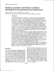
neities under different land–atmosphere boundary flux and water table conditions is warranted for appropriate land surface parameterization in SVAT model grids for different hydroclimatic applications. In this study we investigate both horizontal and vertical soil heterogeneities and address the differences in dealing with both heterogeneities for large-scale hydroclimatic processes. One-dimensional models have been used as approximations of various simplified problems of steady-state water flow across the land–atmosphere boundary (e.g., equilibrium condition between the precipitation events and ignoring other meteorological factors) under investigation. For one-dimensional analyses, two physical scenarios need to be distinguished: 1) vertical layering (heterogeneity), where variations in soil properties are in the vertical directions only (see Fig. 1, bottom) (e.g., Yeh 1989), and 2) vertically homogeneous parallel soil columns with variations of the soil properties in the horizontal plane only (see Fig. 1, top) (e.g., Dagan and Bresler 1983; Bresler and Dagan 1983; Rubin and Or 1993). The objectives of this study with special emphasis on land–atmosphere interaction are twofold: 1) to investigate the impact of the heterogeneous hydraulic soil parameters’ statistics on the pixel-scale effective parameters for both horizontal and vertical heterogeneous conditions under vertically upward/downward steady-state flow scenarios and establish generalized upscaling–aggregation rules based on the requirement that the equivalent medium discharge the mean (evaporation/infiltration) flux of the heterogeneous formation, and 2) to study the significance of the pixel size (domain scale) and the fractal dimensions of the soil hydraulic parameter fields with nested spatial structure on the effective parameters.

2. Methods a. Steady-state one-dimensional flow The unsaturated hydraulic conductivity (K )-capillary pressure head (␺) relationship is represented by the Gardner model (Gardner 1958) K ⫽ Kse⫺␣␺,

共1兲

where Ks is the saturated hydraulic conductivity and ␣ is the pore-size distribution parameter inversely related to the bubbling pressure. In this study, we define a dimensionless form of ␣, ␣* ⫽ ␣L where L is the distance to the water table from the soil surface. By using ␣*, we account for the variations in soil texture (e.g., sand, silt, clay) and groundwater table depth (e.g., deep water table in a desert environment, shallow water table in an agricultural landscape) conditions together

FIG. 1. Schematic view of hydraulic parameter heterogeneity: (top) horizontal (areal) heterogeneity; (bottom) vertical heterogeneity.

during the effective parameter(s) estimation and scaling analyses described later. The other widely used hydraulic conductivity functions can be used as well (e.g., van Genuchten 1980). Our extensive simulations indicated that while the calculated effective parameters using the van Genuchten hydraulic conductivity function differ quantitatively from those using the Gardner function, they follow the same trend and the conclusion reached for the Gardner function also applies for the van Genuchten model.

718


Therefore, we only present analysis using Gardner function in this study without loosing the generality of the approach for adoption to other soil hydraulic functions. Applying Darcy’s law, general equation relating pressure head and elevation above the water table for steady-state vertical flows can be expressed as (e.g., Zaslavsky 1964; Warrick and Yeh 1990) zi⫹1 ⫺ zi ⫽

冕

␺i⫹1

␺i

Ki⫹1共␺兲 d␺, Ki⫹1共␺兲 ⫹ q

共2兲

where zi and zi⫹1 (zi⫹1 ⬎ zi) are the vertical distances above the water table, ␺i and ␺i⫹1 are the suction head at zi and zi⫹1, respectively, Ki⫹1(␺) is the hydraulic conductivity function between zi and zi⫹1, and q is the steady-state evaporation (positive) or infiltration (negative) rate.

b. Heterogeneous hydraulic parameter fields Given the values of mean and coefficient of variation (CV) for the soil hydraulic parameters Ks (具Ks典 and CVK respectively), and ␣* (具␣*典 and CVA respectively), the cross-correlated random fields of Ks and ␣* are generated using the spectral method proposed by Robin et al. (1993). Random fields are produced with the power spectral density function, which was based on exponentially decaying covariance functions. As an indicator of correlation between the two random parameter fields, we used the coherency spectrum given by R共f兲 ⫽

␾12共f兲关␾11共f兲␾22共f兲兴1Ⲑ2

,

共3兲

where ␾11(f), ␾22(f) are the power spectra of random fields 1 and 2, respectively, and ␾12(f) is the cross spectrum between fields 1 and 2. The norm of the coherency spectrum, |R|2, may range from 0 to 1, with |R |2 ⫽ 1 (i.e., the correlation coefficient ␳ ⫽ 1 in the physical domain) indicating a perfect linear correlation between the two random fields. In this study, we used |R |2 ⫽ 1 considering the fact that the value of |R |2 did not significantly alter the results based on our previous/current work. Also, the parameters Ks and ␣* are assumed to obey the lognormal distributions as observed by others in the past (Smith and Diekkruger 1996; Nielsen et al. 1973). Random fields of 10 000 (for a 100 ⫻ 100 grid) for horizontal heterogeneity and 100 (for 100 layers) for vertical heterogeneity are generated. Using this approach, more or less (random) data points do not have significant impact on the effective parameters as long as the mean, variance, and correlation structure remain the same. In other words, 10 000 (100 ⫻ 100) data

VOLUME 8

points for horizontal heterogeneity scenario and 100 points for vertical heterogeneity scenario are proven to be enough in a statistical sense. As the mean value of Ks does not affect the effective hydraulic parameters (demonstrated later), we can use any values for the mean Ks in this study. For the purpose of illustrating our more generalized methodology in terms of a specific example, we use two values of 具␣*典 ⫽ 6 and 1 in generating the random field for ␣*. To give a perspective of how these values relate to actual field soil conditions, we adopt a typical value for silty clay loam ␣ ⫽ 0.01 (1 cm⫺1) from Carsel and Parrish (1988). Combining 具␣*典 ⫽ 6 or 具␣*典 ⫽ 1 and ␣ ⫽ 0.01 (1 cm⫺1) will give a water table depth of about 6 or 1 m, respectively. For describing the spatial variabilities of ␣* and Ks, we use ranges for their coefficient of variations (CVA and CVK) of 0–0.572 and 0–0.822, respectively. The maximum values of CVs (i.e., 0.572 for ␣* and 0.822 for Ks) used here illustrate that the upscaling method developed is appropriate for quite large heterogeneous field conditions. While we present results for a few selected mean parameter and variability values (i.e., relating to different field conditions), it does not mean the procedure developed in the study is limited to these conditions and values. For other field conditions, the values of 具␣*典, CVA, and CVK need to be adjusted to correspond to the actual field conditions, and the developed procedure will still apply.

c. Description of flux in horizontally heterogeneous hydraulic parameter field For horizontally heterogeneous soils (Fig. 1a), application of (2) in combination with the Gardner function (1) in each parallel column (denoted by subscript j) results in the following dimensionless form of the water flux rate at the ground surface,

qj ⫽ KSj

1 ⫺ e␣j*共1⫺h兲 e␣j* ⫺ 1

,

共4兲

where ␣* ⫽ ␣L, h ⫽ ␺L/L are the dimensionless ␣ and surface pressure, respectively. The L is the depth of water table, and ␺L is the surface pressure head. Note that in deriving (4) we only consider horizontal heterogeneity, that is, the hydraulic parameters are constant along the entire profile from the water table to the soil surface with values of Ksj and ␣j*. Using (4) and the generated random fields of Ks and ␣*, we can calculate the flux for each parallel soil column j, and then the mean flux q is calculated by averaging over all the individual column fluxes.

AUGUST 2007

719

MOHANTY AND ZHU

d. Description of flux in vertically heterogeneous hydraulic parameter field Using Gardner’s model, pressure head distribution across a vertically heterogeneous (layered) porous medium (Fig. 1b) can be obtained from (2):

␺*i⫹1 ⫽ ⫺

再

1 q * * * * ln e⫺␣i⫹1共zi ⫹1⫺zi ⫹␺i 兲 ⫺ ␣i⫹1 * Ksi⫹1

冎

⫻ 关1 ⫺ e⫺␣i⫹1共zi⫹1⫺zi 兲兴 . *

*

*

共5兲

Given the generated random fields of Ks and ␣* in the vertical direction and the pressure head condition at the soil surface, h, the flux q can be calculated iteratively from (5) that will satisfy the boundary condition. Setting some initial guess for the water flux in the soil profile q, the iteration procedure starts at the water table (i.e., z0 ⫽ 0 and ␺0* ⫽ 0) and moves upward until it calculates the pressure head at the soil surface. The procedure is repeated by adjusting the value of q according to the calculated surface pressure head in the previous iterations until the calculated surface pressure at the soil surface matches the given boundary condition. The parallel stream-tube type approach presented in this study covers an entire range of steady-state vertical infiltration and evaporation conditions [i.e., the maximum steady-state dimensionless infiltration (q/Ks) is ⫺1 and the maximum steady-state dimensionless evaporation rate is over 0.9]. This wide range of parameter values and flux conditions theoretically correspond to different real-world hydroclimatic scenarios under steady-state conditions typically encountered or approximated between the precipitation events.

e. Effective hydraulic parameter coefficients Since predicting the mean flux rate (evaporation or infiltration) is usually a major focus of most practical soil–vegetation–atmospheric transfer studies, we use a simple approach to derive “effective” hydraulic parameters by assuming that the equivalent homogeneous medium will discharge the same amount of moisture flux across the soil surface as the heterogeneous medium. The effective hydraulic parameters are calculated iteratively from the following equation: 1 ⫺ e␣eff共1⫺h兲 *

Kseff

e␣eff ⫺ 1 *

⫽ qeff,

共6兲

where qeff is the effective flux, qeff ⫽ q for horizontal heterogeneity case, and qeff ⫽ q for vertical heteroge* are the effective paramneity case. Here Kseff and ␣eff

eters for Ks and ␣*, respectively. The left-hand side of * ). In other words, using the effective (6) is q(Kseff, ␣eff hydraulic parameters will produce the same mean flux exchange between the subsurface and the atmosphere. For both horizontal and vertical heterogeneous scenarios, we defined the coefficient of effective parameters for Ks and ␣* as a measure of how close the effective parameter is to the arithmetic mean, respectively, ECK ⫽

KSeff , 具Ks典

共7兲

ECA ⫽

␣eff * , 具␣*典

共8兲

where 具Ks典 is the arithmetic mean of Ks and 具␣*典 is the arithmetic mean of ␣*. Therefore, a coefficient of effective parameter of 1 means an arithmetic mean is appropriate as an effective parameter that will discharge the mean flux over the entire heterogeneous region. As we mentioned earlier, this study focuses only on estimating effective parameters based on matching the mean surface flux (evaporation or infiltration) irrespective of the soil water content or pressure profile distribution. Since there are two effective hydraulic param* ) in one equation [see (6)], in the eters (Kseff and ␣eff following discussion we set one of the effective parameter as the arithmetic mean and find the other effective parameter according to Eq. (6).

3. Heterogeneity effect on effective hydraulic parameters The mean value of Ks does not alter effective parameters because of its linear relationship with the vertical flux. On the other hand, for illustrating the impact of nonlinearity of subsurface flow we used two mean values of the shape parameter 具␣*典 (6.0 and 1.0, representing a most sensitive ␣* range) and two values of surface pressure h (h ⫽ 2.0 for evaporation and h ⫽ 0.1 for infiltration). Note, however, while these mean parameter values are chosen for demonstrating the results across the most sensitive ranges of the selected parameter(s), our methodology encompasses many possible soil hydrologic conditions reflecting real-world scenarios. To put these two values of 具␣*典 in a practical perspective, we use typical values for the hydraulic parameters estimated by Carsel and Parrish (1988) across the soil textural range between sand and clay. The 具␣*典 values of 1.0 and 6.0 translate into a range between 2.8 and 480 cm for the water table depth. Our simulations indicate that a water table depth below 2.8 cm and above 480 cm does not significantly affect the effective

720


VOLUME 8

FIG. 2. Effective coefficient of Ks (ECK) vs coefficient of variation of Ks (CVK) for vertical heterogeneity when only Ks is heterogeneous.

parameter values when compared with the results for 2.8 cm or for 480 cm. It is noteworthy that as we develop a generalized method with dimensionless parameter 具␣*典 and use the values from literature (e.g., Carsel and Parrish 1988) for demonstration purpose, the actual values of 具␣*典 should be determined based on the measured 具␣典 and groundwater table depth at a particular site of applications.

a. When one parameter is heterogeneous 1) KS

HETEROGENEOUS,

␣*

HOMOGENEOUS

For the horizontal heterogeneity case, since the relationship between the surface flux and Ks is linear, the effective Ks in this case would be simply the arithmetic mean of the Ks field. In other words, the effective coefficient of Ks (ECK) is 1. For the vertical heterogeneity case, Fig. 2 shows the ECK versus the coefficient of variation of the Ks field (CVK). Results show that ECK decreases monotonically as the variance of the Ks field increases. It is virtually independent of the surface pressure head condition and mean ␣* values. The ECK is always smaller than 1, indicating that the vertically heterogeneous medium is always more limiting to moisture flux than a homogeneous medium with an arithmetic mean Ks value. It is also important to note that direction of flux (infiltration or evaporation) has no influence on the ECK for vertically heterogeneous medium.

2) ␣*

HETEROGENEOUS,

KS

HOMOGENEOUS

Figure 3 shows the effective coefficient of ␣* (ECA) versus the coefficient of variation of ␣* (CVA) when only the ␣* field is heterogeneous (with homogeneous

FIG. 3. Effective coefficient of ␣* (ECA) vs coefficient of variation of ␣* (CVA) when only ␣* is heterogeneous and 具␣*典 ⫽ 6.0. (a) Horizontal heterogeneity and (b) vertical heterogeneity.

Ks). Figure 3a is for the case of horizontal heterogeneity while Fig. 3b is for the case of vertical heterogeneity. For the sake of brevity, we only present the results for the case of relatively large mean ␣*, 具␣*典 ⫽ 6.0. The results for the case of small mean ␣* are not shown here. Generally, results for smaller 具␣*典 also follow a similar pattern, but in the case of significant differences in the patterns for small versus large values of 具␣*典, the changes will be reported in qualitative terms in the discussion that follows. For the horizontal heterogeneity case, results show that ECA is generally smaller than 1, indicating that the horizontally heterogeneous ␣* generally favors a larger mean surface flux exchange with the atmosphere. For the vertical heterogeneity case, results show that ECA is always larger than 1, indicating that the vertically heterogeneous ␣* generally limits the surface flux exchange with the atmosphere. The variability of the ␣* field causes ECA to be farther away from 1 for evaporation as compared with infiltration;

AUGUST 2007

MOHANTY AND ZHU

721

FIG. 4. Effective coefficient of Ks (ECK) when both Ks and ␣* are heterogeneous and 具␣*典 ⫽ 6.0. (a) Horizontal heterogeneity, h ⫽ 0.1 (i.e., infiltration); (b) horizontal heterogeneity, h ⫽ 2.0 (i.e., evaporation); (c) vertical heterogeneity, h ⫽ 0.1 (i.e., infiltration); and (d) vertical heterogeneity, h ⫽ 2.0 (i.e., evaporation).

that is, the heterogeneous effect is more significant for the evaporation case. Our results also indicate that the heterogeneity has more significant impact when the mean ␣* is larger (i.e., relatively deep water table) compared to the smaller mean ␣* (i.e., relatively shallow water table).

b. When both Ks and ␣* are heterogeneous 1) FINDING ECK MEAN FOR ␣*

WHILE USING ARITHMETIC

Figure 4 presents distributions for ECK as functions of CVK and CVA when both Ks and ␣* are heterogeneous under different flow scenarios and variability orientations. Figures 4a,b are for the case of horizontal heterogeneity, and Figs. 4c,d are for corresponding vertical heterogeneity scenarios with 具␣*典 ⫽ 6.0. Figures 4a,c are for the infiltration scenario (h ⫽ 0.1), and Figs. 4b,d are for the evaporation scenario (h ⫽ 2.0). For the case in Fig. 4a, ECK is close to 1. In other words, horizontal variability in both Ks and ␣* has relatively insignificant influence on ECK for infiltration. A homogeneous medium with arithmetic mean values of Ks and ␣* would be a good equivalent for the corresponding

horizontal heterogeneous system. But quantitatively speaking, both variances (of Ks and ␣*) make ECK smaller and usually farther away from the value of 1, indicating that the heterogeneous system deviates more from mean behavior and discharges less than the equivalent system with arithmetic mean parameters. In other words, the effective parameter leads to arithmetic mean (i.e., gets closer to 1) as both CVK and CVA decrease, reflecting a more homogeneous soil medium. For the evaporation scenario (Fig. 4b), however, ECK behaves differently and is mainly dominated by the ␣* variance. Results indicate that the ␣* variance significantly increases the surface evaporation as compared to the equivalent system with arithmetic mean hydraulic parameters. From a physical perspective, this result suggests that larger localized evaporative fluxes occur because of nonlinear unsaturated hydraulic conductivity distribution across the land–atmosphere interface under relatively deep water table conditions. Figures 4c,d are for the case of vertical heterogeneity and matching hydrologic scenarios as for the horizontal heterogeneity case. Results show that for the infiltration scenario (Fig. 4c) ECK is dominated by the Ks variability. When the flow scenario switches from infiltration (Fig. 4c) to evaporation (Fig. 4d), ECK is

722


VOLUME 8

FIG. 5. Effective coefficient of ␣* (ECA) when both Ks and ␣* are heterogeneous and 具␣*典 ⫽ 6.0. (a) Horizontal heterogeneity, h ⫽ 0.1 (i.e., infiltration); (b) horizontal heterogeneity, h ⫽ 2.0 (i.e., evaporation); (c) vertical heterogeneity, h ⫽ 0.1 (i.e., infiltration); and (d) vertical heterogeneity, h ⫽ 2.0 (i.e., evaporation).

mainly dictated by the ␣* variability. For the vertical heterogeneity scenario, ECK is always smaller than 1. In other words, the vertical heterogeneity of hydraulic parameters always limits moisture flux both downward and upward when compared with the equivalent medium with the arithmetic mean hydraulic parameters. For the evaporation scenario (Fig. 4d), the evaporative flux for the vertically heterogeneous formation is severely limited where ECK approached zero. Physically this may reflect a scenario of a desert environment with a deep groundwater table overlain by layers of lowconductive geological materials. Based on simulations for a number of 具␣*典 values, it has been found that ECK evolved from being entirely CVK dominated for relatively shallow water table (small mean ␣*) and infiltration scenario to being mainly CVA dictated at relatively deep water table (large mean ␣*) and evaporation scenario.

2) FINDING ECA MEAN FOR KS

WHILE USING ARITHMETIC

For a particular porous medium, while Ks determines the magnitude of (maximum) flux (at saturation), ␣* governs the flux across the soil water pressure range during wetting or drying events. It can be shown that the flux decreases approximately exponentially as the value of ␣* increases, and increases linearly with the increasing Ks. Figure 5 shows the results for ECA as functions of CVK and CVA when both Ks and ␣* are

considered heterogeneous fields. Figures 5a,b are for the case of horizontal heterogeneity, while Figs. 5c,d are for the case of vertical heterogeneity. All inputs are the same between Figs. 4 and 5. Compared with Fig. 4, contour maps in Fig. 5 follow a very similar pattern with an inverse numerical sequence for all the corresponding scenarios. Smaller ECA corresponds to higher ECK and vice versa for the same heterogeneity orientation and hydrologic scenarios.

4. Scale effects on effective hydraulic parameters Field observations sometimes indicated that soil hydraulic properties may be correlated over large scales and their variance increases over domain scales (e.g., Hewett 1986; Molz and Boman 1993; Wheatcraft et al. 1990; Wheatcraft and Tyler 1988). Next, we will examine the effects of these features on the effective hydraulic parameters. We first look at the influence of the correlation scales of the hydraulic parameters by comparing the results for the correlation lengths (␰) of 5 and 100 times of the grid spacing using an exponentially decayed covariance function. Figure 6 shows the effective coefficients as functions of the dimensionless surface pressure head at the two different correlation lengths of the random hydraulic parameter fields for CVK ⫽ 0.8225 and CVA ⫽ 0.572. These large CVK and CVA values were selected to investigate the influence of Ks and ␣* variability. Note, however, that while these large values are only chosen to show the signa-

AUGUST 2007

MOHANTY AND ZHU

723

FIG. 6. Effective coefficients vs dimensionless surface pressure head at different correlation lengths of random hydraulic parameter fields. (a) ECK, horizontal heterogeneity; (b) ECA, horizontal heterogeneity; (c) ECK, vertical heterogeneity; and (d) ECA, vertical heterogeneity. In the figure legends, ␰ denotes the ratio of the correlation length of the random fields over the grid length used to generate the random fields.

tures more prominently, result patterns remain unchanged for smaller CVK and CVA. Results demonstrate that the impact of the parameter correlation lengths on the effective coefficients is not significant for all scenarios. Both ECK and ECA are slightly different in value and follow the same trend at significantly different hydraulic parameter correlation lengths (i.e., ␰ ⫽ 5, 100). Overall, for the case of vertical heterogeneity, the impact of the correlation length is more significant than for the case of horizontal heterogeneity. Generally, the influence of the correlation length on effective hydraulic parameters is relatively insignificant compared with other inputs, such as the means and variances of the hydraulic parameters. While we have shown that the correlation length is relatively insignificant in influencing the effective hydraulic coefficients, the variances (coefficients of variation) of the hydraulic parameters do influence the effective coefficients significantly. Therefore, the scale impact will be mainly reflected in the increase of variance because of an increasing domain scale. For mathematical simplicity, the soil hydraulic properties in the

horizontal and vertical directions are approximated as fractal phenomena (e.g., Peyton et al. 1994). We assume that the hydraulic parameters obey the fractal Brownian motion statistics for which the spectral density has the form of a power law with the power-law index related to the fractal dimension (e.g., Hassan et al. 1997). While we use the fractal Brownian motion statistics as a way to simplify mathematical description and to relate effective hydraulic parameters to the fractal dimension, the methodology described in this study can be extended to any process where increasing hydraulic parameter variance is related to the domain scale considered. Fractal processes by definition are infinitely correlated, and their variance increases with the scale of the domain asymptotically to infinity. In real systems, the domain boundary will determine the limit of heterogeneity. The maximum domain scale in turn determines the minimum wavenumber (e.g., Zhan and Wheatcraft 1996). If we use the minimum wavenumber cutoff, which is related to the maximum scale of the domain of interest, then the variance (␴2) can be related to the scale X as follows:

724


FIG. 7. Effective coefficient of Ks (ECK) vs relative domain scale (Y ) and fractal dimension of Ks (Dk) for vertical heterogeneity case when only Ks is heterogeneous.

␴2 ⫽

S0X2共2⫺D兲共2 ⫺ D兲共2␲兲2共2⫺D兲

共9兲

,

where S0 is a parameter related to the maximum domain scale, and D is the fractal dimension. If there is a potential maximum domain scale under consideration, Xmax, we can relate X to Xmax as X ⫽ XmaxY, where Y is the dimensionless relative scale. Then the scalerelated variance is as follows: 2 ␴2 ⫽ ␴max Y2共2⫺D兲,

共10兲

where 2 ␴max ⫽

共2⫺D兲 S0X2max

共2 ⫺ D兲共2␲兲2共2⫺D兲

.

共11兲

Using this variance-scale relationship, we can now relate the effective coefficients for the hydraulic parameters to the hierarchical spatial scale structure. Figure 7 shows the results for ECK versus the relative domain scale (Y ) and the fractal dimension of the Ks field (Dk) for the case of vertical heterogeneity when only Ks is heterogeneous. Results show that ECK decreases as either the domain scale or the fractal dimension increases. The increase in both the domain scale and the fractal dimension will shift ECK farther away from 1, indicating an increasing heterogeneous effect.

VOLUME 8

As discussed earlier, ECK for the case of vertical heterogeneity is always smaller than 1; in other words, the vertically heterogeneous system limits moisture fluxes in both upward and downward directions. Figure 8 shows the results for ECA as functions of the relative domain scale and the fractal dimension of the ␣* field (Da) when only the parameter ␣* is heterogeneous. Figures 8a,b are for the case of horizontal heterogeneity and Figs. 8c,d are for the vertical heterogeneity. For the infiltration scenario (Figs. 8a,c), ECA changes slightly within a small range around 1 (i.e., around arithmetic mean). For the evaporation scenario (Figs. 8b,d), the domain scale and the fractal dimension have a more significant influence on ECA. Both the domain scale and the fractal dimension steer ECA away from 1. For the horizontal heterogeneity situation, ECA is generally smaller than 1, suggesting that the horizontal ␣* heterogeneity increases the moisture flux where a larger fractal dimension supports large mean moisture. As mentioned earlier, the vertical heterogeneity constrains/reduces the mean moisture flux (i.e., ECA ⬎ 1), especially for the evaporation scenario. The increasing fractal dimension will further reduce the mean moisture flux both downward and upward as depicted by increased ECA values. Figure 9 illustrates that results for ECK as functions of the relative domain scale (Y ) and the fractal dimension of the Ks field (Dk) when both Ks and ␣* are heterogeneous and CVA ⫽ 0.572. Some of the important observations include large ECK for the case shown in Fig. 9b indicate that a combination of Ks and ␣* heterogeneities greatly increases the mean evaporative flux. For the horizontal heterogeneous situation, a few small ␣*s dominate the moisture flux and greatly increase the mean flux for the heterogeneous formation. Corresponding to Fig. 9b conditions, ECK for the vertical heterogeneity case is very small (see Fig. 9d) where a few large ␣* will severely limit the mean moisture flux. It can be shown that the flux decreases approximately exponentially with the increasing ␣*, and increases linearly with the increasing Ks. Therefore, it can be expected that the ␣* heterogeneity has a more significant impact on the mean moisture flux in the heterogeneous soil formations. It can be observed from our results that the increasing fractal dimension of Ks (Dk) generally steers ECK farther away from 1 and thus increases the heterogeneous effects. Figure 10 displays the results for ECA as functions of the relative domain scale (Y ) and the fractal dimension of the ␣* field (Da) when both Ks and ␣* are heterogeneous and CVK ⫽ 0.822. Results are presented for same hydrologic scenarios and heterogeneity orienta-

AUGUST 2007

MOHANTY AND ZHU

725

FIG. 8. Effective coefficient of ␣* (ECA) vs relative domain scale (Y ) and fractal dimension of ␣* (Da) when only ␣* is heterogeneous and 具␣*典 ⫽ 6.0. (a) Horizontal heterogeneity, h ⫽ 0.1 (i.e., infiltration); (b) horizontal heterogeneity, h ⫽ 2.0 (i.e., evaporation); (c) vertical heterogeneity, h ⫽ 0.1 (i.e., infiltration); and (d) vertical heterogeneity, h ⫽ 2.0 (i.e., evaporation).

tions as in the previous cases. Overall, it can be observed that ECA is generally larger than 1 with the exception of evaporation for horizontal heterogeneity (Fig. 10b). Since we have used the arithmetic mean for the Ks field in calculating ECA, the fact that ECA is mostly greater than 1 and ECK is mostly smaller than 1 (as seen in Fig. 9) indicates that the heterogeneous formation where both Ks and ␣* are heterogeneous discharges generally less than the equivalent homogeneous formations with the arithmetic mean hydraulic parameters. For the infiltration case, ECA is more pre-

dictable, being consistently larger than 1, and both the domain scale and the fractal dimension of ␣* increase ECA. For the evaporation case, our calculations indicate that its trend reverses depending on the value of the mean ␣*. For small mean ␣* (corresponding to a relatively shallow water table), ECA increase as both the scale and the fractal dimension increase, while for large mean ␣* (corresponding to a relatively deep water table), it decreases with the scale and the fractal dimension. Figures 10c,d show the results for the vertical hetero-

726


VOLUME 8

FIG. 9. Effective coefficient of Ks (ECK) vs relative domain scale (Y ) and fractal dimension of Ks (Dk) when both Ks and ␣* are heterogeneous, 具␣*典 ⫽ 6.0 and CVA ⫽ 0.572. (a) Horizontal heterogeneity, h ⫽ 0.1 (i.e., infiltration); (b) horizontal heterogeneity, h ⫽ 2.0 (i.e., evaporation); (c) vertical heterogeneity, h ⫽ 0.1 (i.e., infiltration); and (d) vertical heterogeneity, h ⫽ 2.0 (i.e., evaporation).

geneity. While the vertical heterogeneity of hydraulic parameters always limits both downward and upward moisture fluxes (i.e., ECA is always larger than 1), the influence of the domain scale (Y ) and the fractal dimension of ␣* (Da) is mixed. For the case of infiltration, both the relative domain scale and the fractal dimension of ␣* slightly decrease ECA (Fig. 10c); that is, they decrease the heterogeneity effects. For the case of evaporation, both the relative domain scale and the fractal dimension of ␣* actually increase ECA (Fig. 10d); that is, they increase the heterogeneity effects.

5. Concluding remarks Based on our comprehensive simulations under horizontal and vertical heterogeneity orientation and hydrologic scenarios from the perspective of land–atmosphere interaction modeling, the main conclusions drawn from this study are the following: 1) A vertically heterogeneous variably saturated porous medium does not discharge as much moisture flux as the equivalent homogeneous medium of arithmetic mean values for the (Ks and ␣) hydraulic

AUGUST 2007

MOHANTY AND ZHU

727

FIG. 10. Effective coefficient of ␣* (ECA) vs relative domain scale (Y ) and fractal dimension of ␣* (Da) when both Ks and ␣* are heterogeneous, 具␣*典 ⫽ 6.0 and CVK ⫽ 0.822. (a) Horizontal heterogeneity, h ⫽ 0.1 (i.e., infiltration); (b) horizontal heterogeneity, h ⫽ 2.0 (i.e., evaporation); (c) vertical heterogeneity, h ⫽ 0.1 (i.e., infiltration); and (d) vertical heterogeneity, h ⫽ 2.0 (i.e., evaporation).

parameters. In other words, a vertically heterogeneous subsurface soil is more limiting to soil moisture flux across the land–atmosphere boundary in comparison to a horizontally heterogeneous soil across the landscape. 2) When only the Ks field is heterogeneous, the concept of effective coefficient of Ks works the best. For the case of horizontal heterogeneity, ECK is simply 1, since Ks linearly controls the steady-state moisture flux. For the case of vertical heterogeneity, ECK decreases only with CVK and is virtually in-

dependent of other hydraulic parameters and hydrologic conditions. 3) The heterogeneity of the ␣* field significantly influences ECA and ECK, since it severely limits the flux both upward and downward. 4) For the evaporation scenario the effective coefficients are dictated more by the ␣* heterogeneity, while for the infiltration scenario the effective coefficients are mainly controlled by the Ks variability. 5) In general, increase in both the fractal dimension and the relative domain scale enhances the hetero-

728


geneity effects of parameter fields on the effective coefficients for the hydraulic parameters. The impact of the domain scale on the effective coefficients is more significant as the fractal dimension increases. 6) For the case of vertical heterogeneity, ␣* heterogeneity dominates the effective coefficients, mainly because Ks linearly controls the moisture flux while ␣* dictates the moisture flux in a highly nonlinear manner. A few large or small ␣*s can significantly reduce or enhance flux, both upward and downward. The above findings, along with our past studies (Zhu and Mohanty 2002a,b, 2003a,b, 2004, 2006; Zhu et al. 2004, 2006), will help choose the appropriate equivalent soil hydraulic parameters for distributed SVAT model grids with horizontal and vertical soil heterogeneities. However, further studies are needed to make the proposed parallel stream-tube type approach more comprehensive and realistic in terms of three-dimensional subsurface flow and transient atmospheric boundary conditions. Acknowledgments. This project is funded by NASA (Grants NAG5-11702 and NNG06GH01G) and NSF (DMS-0621113), and is also supported in part by Sustainability of Semi-Arid Hydrology and Riparian Areas (SAHRA) under the STC Program of the National Science Foundation, Agreement EAR-9876800, Los Alamos National Laboratory, the Water Resources Research Act, Section 104 research grant program of the U.S. Geological Survey, DRI’s Applied Research Initiative and start-up fund. REFERENCES Bresler, E., and G. Dagan, 1983: Unsaturated flow in spatially variable fields, 2. Application of water flow models to various fields. Water Resour. Res., 19, 421–428. Brooks, R. H., and A. T. Corey, 1964: Hydraulic properties of porous media. Colorado State University Hydrology Paper 3, 27 pp. Carsel, R. F., and R. S. Parrish, 1988: Developing joint probability distributions of soil water retention characteristics. Water Resour. Res., 24, 755–769. Dagan, G., and E. Bresler, 1983: Unsaturated flow in spatially variable fields, 1. Derivation of models of infiltration and redistribution. Water Resour. Res., 19, 413–420. Desbarats, A. J., 1998: Scaling of constitutive relationships in unsaturated heterogeneous media: A numerical investigation. Water Resour. Res., 34, 1427–1435. Gardner, W. R., 1958: Some steady state solutions of unsaturated moisture flow equations with applications to evaporation from a water table. Soil Sci., 85, 228–232. Gelhar, L. W., and C. L. Axness, 1983: Three-dimensional sto-

VOLUME 8

chastic analysis of macrodispersion in aquifers. Water Resour. Res., 19, 161–180. Harter, T., and D. Zhang, 1999: Water flow and solute spreading in heterogeneous soils with spatially variable water content. Water Resour. Res., 35, 415–426. ——, and J. W. Hopmans, 2004: Role of vadose zone flow processes in regional scale hydrology: Review, opportunities and challenges. Unsaturated Zone Modeling: Processes, Applications, and Challenges, R. A. Feddes, G. H. de Rooij, and J. C. van Dam, Eds., Kluwer, 179–208. Hassan, A. E., J. H. Cushman, and J. W. Delleur, 1997: Monte Carlo studies of flow and transport in fractal conductivity fields: Comparison with stochastic perturbation theory. Water Resour. Res., 33, 2519–2534. Hewett, T. A., 1986: Fractal distribution of reservoir heterogeneity and their influence on fluid transport. Preprints, Annual Technical Conf. and Exhibition, New Orleans, LA, Society of Petroleum Engineers, 1–16. Jenny, H., 1941: Factors of Soil Formation: A System of Quantitative Pedology. McGraw-Hill, 281 pp. Kim, C. P., and J. N. M. Stricker, 1996: Influence of spatially variable soil hydraulic properties and rainfall intensity on the water budget. Water Resour. Res., 32, 1699–1712. ——, ——, and R. A. Feddes, 1997: Impact of soil heterogeneity on the water budget of the unsaturated zone. Water Resour. Res., 33, 991–999. Koster, R. D., and Coauthors, 2004: Regions of strong coupling between soil moisture and precipitation. Science, 305, 1138– 1140. Mohanty, B. P., and Z. Mousli, 2000: Saturated hydraulic conductivity and soil water retention properties across a soil-slope transition. Water Resour. Res., 36, 3311–3324. ——, R. S. Kanwar, and R. Horton, 1991: A robust-resistant approach to interpret spatial behavior of saturated hydraulic conductivity of a glacial till under no-tillage system. Water Resour. Res., 27, 2979–2992. ——, ——, and C. J. Everts, 1994: Comparison of saturated hydraulic conductivity measurement methods for a glacial-till soil. Soil Sci. Soc. Amer. J., 58, 672–677. Molz, F. J., and G. K. Boman, 1993: A fractal-based stochastic interpolation scheme in subsurface hydrology. Water Resour. Res., 29, 3769–3774. Montoglou, A., and L. W. Gelhar, 1987a: Stochastic modeling of large-scale transient unsaturated flow systems. Water Resour. Res., 23, 37–46. ——, and ——, 1987b: Capillary tension head variance, mean soil moisture content, and effective specific soil moisture capacity of transient unsaturated flow in stratified soils. Water Resour. Res., 23, 47–56. ——, and ——, 1987c: Effective hydraulic conductivities of transient unsaturated flow in stratified aquifer. Water Resour. Res., 23, 57–67. Nielsen, D. R., J. W. Biggar, and K. T. Erh, 1973: Spatial variability of field-measured soil-water properties. Hilgardia, 42, 215–260. Peyton, R. L., C. J. Gantzer, S. H. Anderson, B. A. Haeffner, and P. Pfeifer, 1994: Fractal dimension to describe soil macropore structure using X ray computed tomography. Water Resour. Res., 30, 691–700. Robin, M. J. L., A. L. Gutjahr, E. A. Sudicky, and J. L. Wilson,

AUGUST 2007

MOHANTY AND ZHU

1993: Cross-correlated random field generation with the direct Fourier transform method. Water Resour. Res., 29, 2385– 2397. Rubin, Y., and D. Or, 1993: Stochastic modeling of unsaturated flow in heterogeneous soil with water uptake by plant roots: The parallel columns model. Water Resour. Res., 29, 619–631. Russo, D., 1992: Upscaling of hydraulic conductivity in partially saturated heterogeneous porous formation. Water Resour. Res., 28, 397–409. ——, 1993: Stochastic modeling of macrodispersion for solute transport in a heterogeneous unsaturated porous formation. Water Resour. Res., 29, 383–397. ——, 1995a: On the velocity covariance and transport modeling in heterogeneous anisotropic porous formations: 2. Unsaturated flow. Water Resour. Res., 31, 139–145. ——, 1995b: Stochastic analysis of the velocity covariance and the displacement covariance tensors in partially saturated heterogeneous anisotropic porous formations. Water Resour. Res., 31, 1647–1658. Smith, R. E., and B. Diekkruger, 1996: Effective soil water characteristics and ensemble soil water profiles in heterogeneous soils. Water Resour. Res., 32, 1993–2002. van Genuchten, M. Th., 1980: A closed-form equation for predicting the hydraulic conductivity of unsaturated soils. Soil Sci. Soc. Amer. J., 44, 892–898. Warrick, A. W., and T.-C. J. Yeh, 1990: One-dimensional, steady vertical flow in a layered soil profile. Adv. Water Resour., 13, 207–210. Wheatcraft, S. W., and S. W. Tyler, 1988: An explanation of scaledependent dispersivity in heterogeneous aquifers using concepts of fractal geometry. Water Resour. Res., 24, 566–578. ——, G. A. Sharp, and S. W. Tyler, 1990: Fluid flow and solute transport in fractal heterogeneous porous media. Dynamics of Fluids in Hierarchical Porous Media, J. H. Cushman, Ed., Academic Press, 528 pp. Yang, J., R. Zhang, and J. Wu, 1996: An analytical solution of macrodispersivity for adsorbing solute transport in unsaturated soils. Water Resour. Res., 32, 355–362. Yeh, T.-C. J., 1989: One-dimensional steady state infiltration in heterogeneous soils. Water Resour. Res., 25, 2149–2158. ——, L. W. Gelhar, and A. L. Gutjahr, 1985a: Stochastic analysis of unsaturated flow in heterogeneous soils, 1. Statistically isotropic media. Water Resour. Res., 21, 447–456.

729

——, ——, and ——, 1985b: Stochastic analysis of unsaturated flow in heterogeneous soils, 2. Statistically anisotropic media with variable ␣. Water Resour. Res., 21, 457–464. ——, ——, and ——, 1985c: Stochastic analysis of unsaturated flow in heterogeneous soils, 3. Observation and applications. Water Resour. Res., 21, 465–471. Zaslavsky, D., 1964: Theory of unsaturated flow into a nonuniform soil profile. Soil Sci., 97, 400–410. Zhan, H., and S. W. Wheatcraft, 1996: Macrodispersivity tensor for nonreactive solute transport in isotropic and anisotropic fractal porous media: Analytical solutions. Water Resour. Res., 32, 3461–3474. Zhang, D., T. C. Wallstrom, and C. L. Winter, 1998: Stochastic analysis of steady-state unsaturated flow in heterogeneous media: Comparison of the Brooks–Corey and Gardner– Russo models. Water Resour. Res., 34, 1437–1449. Zhu, J., and B. P. Mohanty, 2002a: Upscaling of hydraulic properties for steady state evaporation and infiltration. Water Resour. Res., 38, 1178, doi:10.1029/2001WR000704. ——, and ——, 2002b: Spatial averaging of van Genuchten hydraulic parameters for steady-state flow in heterogeneous soils: A numerical study. Vadose Zone J., 1, 261–272. ——, and ——, 2003a: Effective hydraulic parameters for steady state vertical flow in heterogeneous soils. Water Resour. Res., 39, 1227, doi:10.1029/2002WR001831. ——, and ——, 2003b: Upscaling of hydraulic properties in heterogeneous soils. Scaling Methods in Soil Physics, Y. Pachepsky, D. E. Radcliffe, and H. M. Selim, Eds., CRC Press, 97– 117. ——, and ——, 2004: Soil hydraulic parameter upscaling for steady state flow with root water uptake. Vadose Zone J., 3, 1464–1470. ——, and ——, 2006: Effective scaling factor for transient infiltration in heterogeneous soils. J. Hydrol., 319, 96–108. ——, ——, A. W. Warrick, and M. Th. van Genuchten, 2004: Correspondence and upscaling of hydraulic functions for steady-state flow in heterogeneous soils. Vadose Zone J., 3, 527–533. ——, ——, and N. N. Das, 2006: On the effective averaging schemes of hydraulic properties at the landscape scale. Vadose Zone J., 5, 308–316.