Effective Modified Hybrid Conjugate Gradient Method ...

Available at http://pvamu.edu/aam Appl. Appl. Math. ISSN: 1932-9466 Vol. 12, Issue 2 (December

Applications and Applied Mathematics: An International Journal (AAM)

2017), pp. 1036 - 1056

Effective Modified Hybrid Conjugate Gradient Method for Large-Scale Symmetric Nonlinear Equations 1

Jamilu Sabi'u and 2Mohammed Yusuf Waziri 1

Department of Mathematics Faculty of Science Northwest University Kano Kano, Nigeria [email protected]

2

Department of Mathematical Sciences Faculty of Science Bayero University Kano Kano, Nigeria [email protected]

Received: December 2, 2016; Accepted: September 2, 2017

Abstract In this paper, we proposed hybrid conjugate gradient method using the convex combination of FR and PRP conjugate gradient methods for solving Large-scale symmetric nonlinear equations via Andrei approach with nonmonotone line search. Logical formula for obtaining the convex parameter using Newton and our proposed directions was also proposed. Under appropriate conditions global convergence was established. Reported numerical results show that the proposed method is very promising.

Keywords: Backtracking line search; Secant equation; symmetric nonlinear equations; Conjugate gradient method

MSC 2010: 90C30, 65K05, 90C53, 49M37, 15A18 1. Introduction Let us consider the systems of nonlinear equations

1036

AAM: Intern. J., Vol. 12, Issue 2 (December 2017)

1037

F (x) = 0,

(1)

where F : R n  R n is a nonlinear mapping. Often, the mapping, F is assumed to satisfy the following assumptions: A1. A2. A3. A4.

There exists an x *  R n s.t F ( x* ) = 0 . F is a continuously differentiable mapping in a neighborhood of x * . F ( x* ) is invertible. The Jacobian F ' ( x ) is symmetric.

The prominent method for finding the solution of (1) is the classical Newton's method which generates a sequence of iterates {xk } from a given initial point x0 via xk 1 = xk  ( F ' ( xk )) 1 F ( xk ),

(2)

where k = 0,1,2 . The attractive features of this method are rapid convergence, and ease of implementation. Nevertheless, Newton's method requires the computation of the Jacobian matrix, which requires the first-order derivative of the systems. In practice, computations of some function’s derivatives are quite costly and sometimes they are not available or could not be done precisely. In this case Newton's method cannot be applied directly. In this work, we are interested in handling large-scale problems for which the Jacobian is either not available or requires a low amount of storage. The best method is CG approach. It is vital to mention that the conjugate gradient methods are among the popular used methods for unconstrained optimization problems. They are particularly efficient for handling large-scale problems due to their convergence properties, simplicity to implement and low storage (Zhou and Shen(2015)). Not withstanding, the study of conjugate gradient methods for large-scale symmetric nonlinear systems of equations is scanty, and this is what motivated us to have this paper. In general, CG methods for solving nonlinear systems of equations generate an iterative points {xk } from initial given point x0 using xk 1 = xk   k d k , (3) where  k > 0 is attained via line search, and directions d k are obtained using

if k = 0,  F ( xk ), dk =    F ( xk )   k d k , if k  1,

(4)

 k is term as conjugate gradient parameter. This problem under study may arise from an unconstrained optimization problem, a saddle point problem, Karush-Kuhn-Tucker (KKT) of equality constrained optimization problem, the discritized two-point boundary value problem, the discritized elliptic boundary value problem, and

Jamilu Sabi’u and Mohammed Yusuf Waziri

1038

etc. Equation (1) is the first-order necessary condition for the unconstrained optimization problem when F is the gradient mapping of some function, f : Rn  R min f ( x),

x  Rn .

(5)

For the equality constrained problem min f ( x), s.t h( z ) = 0,

(6)

where h is a vector-valued function. The KKT conditions can be represented as the system (1) with x = ( z, v), and F ( z, v) = (F ( z )  h( z )v, h( z )),

(7)

where v is the vector of Lagrange multipliers. Notice that the Jacobian F ( z, v) is symmetric for all ( z , v ) (see, e.g., (Ortega and Rheinboldt (1970)). Problem (1) can be converted to the following global optimization problem (5) with our function f defined by f ( x) =

1 || F ( x) || 2 . 2

(8)

A large number of efficient solvers for large-scale symmetric nonlinear equations have been proposed, analyzed, and tested in the last decade. Among them the most classic one entirely due to (Li and Fukushima (1999)), in which a Gauss-Newton-based BFGS method is developed. The global and superlinear convergence are also established. Its performance is further improved by (Gu et al. (2002)), where a norm descent BFGS method is designed. Norm descent type BFGS methods especially coorporating with trust regions strategy are presented in the literature which showed their moderate effectiveness experimentally (Yuan et al. (2009)). Still the matrix storage and solving of n-linear systems are required in the BFGS type methods presented in the literature. The recent designed nonmonotone spectral gradient algorithm (Cheng and Chen (2013)) falls within the frame work of matrix-free. The conjugate gradient methods for symmetric nonlinear equations has received a good attention and taken an appropriate progress. However, (Li and Wang (2011)) proposed a modified Flectcher-Reeves conjugate gradient method which is based on the work of (Zhang et al. (2006)), and the results illustrate that their proposed conjugate gradient method is promising. In line with this development, further studies on conjugate gradient are inspired for solving large-scale symmetric nonlinear equations. (Zhou and Shen (2014)) extended the descent three-term polak-Rebiere-Polyak of (Zhang et al. (2006)) for solving (1) by combining with the work of (Li and Fukushima (1999)). Meanwhile the classic polak-Rebiere-Polyak is successfully used to solve symmetric Equation (1) by (Zhou and Shen (2015)). Subsequentely (Xia, et al.(2015)) proposed a method based on well-known conjugate gradient of (Hager and Zhang (2005)). The proposed method converges globally. Extensive numerical

AAM: Intern. J., Vol. 12, Issue 2 (December 2017)

1039

experiments showed that each over-mentioned method performs quite well. Some related papers on symmetrics nolinear systems are (Romero-Cadava et al, (2013), Sabi'u (2017), Sabi'u and Sanusi (2016) and Waziri and Sabi'u (2016)). In this work, we propose to present a hybrid CG method using FR and PRP CG parameters. Our anticipation is to suggest a good CG parameter that will lead to a solution with less computational cost. We organized the paper as follows: In the next section, we present the details of the proposed method. Convergence results are presented in Section 3. Some numerical results are reported in Section 4. Finally, conclusions are made in Section 5.

2. Effective Modified Hybrid CG Method (MHCG) This section presents effective modified hybrid conjugate gradient method (FR and PRP) using some fundamental approach of (Andrei (2008)) by incorporating the nonnegative restriction of the CG parameter suggested by (Powell (1984)). We are motivated by the work of (Li and Fukushima (1999)), i.e., globally and superlinearly Gauss-Newton-based BFGS method for symmetric nonlinear system. In their work, an approximate gradient is obtained without taking the derivative, i.e., gk =

F ( x k   k Fk )  Fk

k

(9)

,

and the search direction d k is produced by solving the linear equations Bk d k =  g k . where  k is the stepsize to be obtained by some line search, and the matrix Bk is updated by the BFGS formula

Bk 1 = Bk 

Bk s k s kT Bk y k y kT  T . s kT Bk s k yk sk

In view of the above fact, we further present the convex combination of FR and PRP conjugate gradient methods to obtain:

 kH * = (1   k ) kFR   k  kPRP ,

(10)

where

kFR =

|| f ( xk 1 ) ||2 f ( xk 1 )T yk PRP ,  = k || f ( xk ) ||2 || f ( xk ) ||2

and

yk = f ( xk 1 )  f ( xk ),

 k is a scalar satisfying 0   k  1 . By substituting (11) in to (10) we have

(11)

Jamilu Sabi’u and Mohammed Yusuf Waziri

1040



H* k

|| f ( xk 1 ) || 2 f ( xk 1 ) T y k = (1   k ) k . || f ( xk ) || 2 || f ( xk ) || 2

(12)

Using (4) and (12), our new direction becomes:

d k 1 = f ( xk 1 )  (1   k )

|| f ( xk 1 ) || 2 f ( xk 1 ) T y k d   dk , k k || f ( xk ) || 2 || f ( xk ) || 2

(13)

or equvalently,

|| f ( xk 1 ) || 2 f ( xk 1 )T yk d k 1 = f ( xk 1 )  (1   k ) sk   k sk . || f ( xk ) || 2 || f ( xk ) || 2

(14)

However, in order to guarantee a good selection of  k , k , we equate the Newton direction with our proposed direction, due to the fact that "It is remarkable that if the point xk 1 is close enough to a local minimizer x * , then a good direction to follow is the Newton direction"

 J 1f ( xk 1 ) = f ( xk 1 )  (1   k )

|| f ( xk 1 ) || 2 f ( xk 1 ) T y k s   sk , k k || f ( xk ) || 2 || f ( xk ) || 2

(15)

to get

|| f ( xk 1 ) || 2 || f ( xk 1 ) || 2 f ( xk 1 ) T y k  J f ( xk 1 ) = f ( xk 1 )  sk   k sk   k sk . || f ( xk ) || 2 || f ( xk ) || 2 || f ( xk ) || 2 1

(16) It is well-known that || f ( xk 1 ) || = f ( xk 1 ) f ( xk 1 ) , Therefore we obtain 2

 J 1f ( xk 1 ) = f ( xk 1 ) 

T

|| f ( xk 1 ) || 2 f ( xk 1 ) T ( y k  f ( xk 1 )) s   sk . k k || f ( xk ) || 2 || f ( xk ) || 2

(17)

By the definition of yk = f ( xk 1 )  f ( xk ) we arrive at

|| f ( xk 1 ) || 2 f ( xk 1 ) T f ( xk )  J f ( xk 1 ) = f ( xk 1 )  sk   k sk . || f ( xk ) || 2 || f ( xk ) || 2 1

(18)

Multiplying (18) by J k 1skT , we have

 s kT f ( xk 1 ) =  J k 1 s kT f ( xk 1 )  J k 1 s kT

T || f ( xk 1 ) || 2 T f ( x k 1 ) f ( x k ) s   J s sk , k k k 1 k || f ( xk ) || 2 || f ( xk ) || 2

(19)

AAM: Intern. J., Vol. 12, Issue 2 (December 2017)

1041

and hence, after some algebraic manipulations, we have || f ( x k 1 ) || 2 T s k J k 1 s k || f ( x k ) || 2 . f ( x k 1 )) T f ( x k ) T s k J k 1 s k || f ( x k ) || 2

s kT f ( x k 1 )  s kT J k 1f ( x k 1 ) 

k =

(20)

Due to the essential property of low memory requirements for the CG methods, we apply the modified secant equation proposed by (Babaie-Kafaki and Ghanbari (2014)),

J k11 y k = 2

|| y k || 2 sk , s kT y k

(21)

or, equivalently

1 s kT y k J k 1 s k = yk = zk . 2 || y k || 2

(22)

Substituting (22) into (20) we obtained the following hybridization parameter

k =

( sk  zk )T f ( xk 1 ) || f ( xk ) || 2  zkT sk || f ( xk 1 ) || 2 . zkT sk f ( xk 1 )T f ( xk )

(23)

Replacing the terms f ( xk 1 ) and f ( xk ) by g k 1 and g k in (9) respectively, yield

( sk  zk )T g k 1 || g k || 2  zkT sk || g k 1 || 2 k = , sk = xk 1  xk . zkT sk g kT1 g k

(24)

Having derived the CG parameter (  kH * ) in (10), we then present our direction as d 0 =  g ( x0 ),

d k 1 =  g k 1   kH * d k ,

k = 1,2,

(25)

where

 kH * = (1   k ) kFR   k  kPRP , and  k

(26)

given by (24) with

 kFR =

|| g k 1 || 2 , || g k || 2

 kPRP =

g kT1 yk || g k || 2

and

yk = g k 1  g k .

(27)

Jamilu Sabi’u and Mohammed Yusuf Waziri

1042

It is vital to note that, the hybridization parameter  k given by (24) may be outside the interval [0,1]. However, in order to have convex combination in (26), we adopt the consideration of (Andrei 2008)) in the sense that if  k < 0 , then we let  k = 0 , and if  k > 1 , then we let  k = 0 . Finally, we present our scheme as xk 1 = xk   k d k .

(28)

Moreover, the direction d k given by (25) may not be a descent direction of (8), in which case the standard wolfe and Armijo line searches cannot be used to compute the stepsize directly. Therefore, we use the nonmonotone line search proposed in (Zhou and Shen (2014)) to compute our stepsize  k . Let 1 > 0 , 2 > 0 , r  (0,1) be constants and  k  be a given positive sequence such that 



k

< .

(29)

k =0

Let  k = max 1, r k  satisfy f ( xk   k d k )  f ( xk )  1 ||  k F ( xk ) || 2 2 ||  k d k || 2 k f ( xk ).

(30)

Now, we can describe the algorithm for our proposed method as follows:

Algorithm (MHCG) Step 1 : Step Step Step Step Step

2: 3: 4: 5: 6:

Given x0 ,  > 0 ,   (0,1) , r  (0,1) and a positive sequence  k satisfying (29), and set k = 0 . Test a stopping criterion. If yes, then stop; otherwise continue with Step 3. Compute d k by (25). Compute  k by the line search (30). Compute xk 1 = xk   k d k . Consider k = k  1 and go to step 2.

3. Convergence Result This section presents global convergence results of hybrid CG method. To begin with, let us define the level set as: (31)  = x | f ( x)  e n f ( x0 ). To analyze the convergence of our method, we will make the following assumptions on nonlinear systems (1).

AAM: Intern. J., Vol. 12, Issue 2 (December 2017)

1043

Assumption 1 (i) The level set  defined by (31) is bounded. (ii) There exists x*   such that F ( x* ) = 0 , F (x ) is continuous for all x . (iii) In some neighborhood N of  , the Jacobian is Lipschitz continous, i.e there exists a positive constant L > 0 such that F ( x)  F ( y )  L x  y ,

(32)

for all x, y  N . Properties (i) and (ii) imply that there exists positive constants M1 , M 2 and L1 such that

|| F ( x) || M1 , || J ( x) || M 2 , xN ,

(33)

|| f ( x)  f ( y) || L1 || x  y ||, || J ( x) || M 2 , x, y  N .

(34)

Lemma 1.1. (Zhou and Shen (2014)) Let the sequence xk  be generated by the algorithms above. Then the sequence || Fk || converges and xk  N for all k  0 . Lemma 1.2. Let the properties of (1) above hold. Then we have lim ||  k d k ||= lim || sk ||= 0,

(35)

lim ||  k Fk ||= 0.

(36)

k 

k 

k 

Proof: By (29) and (30) we have for all k > 0 ,

2 ||  k d k || 2  1 ||  k F ( xk ) || 2 2 ||  k d k || 2 || Fk || 2  || Fk 1 || 2  k || Fk || 2 .

(37)

By summing the above k inequality, we obtain k



k



 2  ||  k d k || 2 || Fk || 2 (1   i ) || Fk 1 || 2 . i =0

 i =0



(38)

Jamilu Sabi’u and Mohammed Yusuf Waziri

1044

From (33) and the fact that  k  satisfies (29), the series



k

i =0

||  k d k || 2 is convergent. This

implies (35). By a similar way, we can prove that (36) holds. The following result shows that Modified hybrid CG method algorithm is globally convergent. Theorem 1.1. Let the properties of (1) above hold. Then the sequence xk  generated by Modified hybrid CG method algorithm converges globally; that is, liminf || f ( xk ) ||= 0.

(39)

k 

Proof: We prove this theorem by contradiction. Suppose that (39) is not true, then there exists a positive constant  such that || f ( xk ) ||  , k  0.

(40)

Since f ( xk ) = J k Fk , (40) implies that there exists a positive constant  1 satisfying || Fk ||  1 , k  0.

(41)

Case (i):

limsup k    k > 0. Then by (36), we have liminf

k 

|| Fk ||= 0 . This and Lemma (1.1.) show that

lim k   || Fk ||= 0 , which contradicts (40).

Case (ii): limsup k    k = 0 . Since  k  0 , this case implies that lim  k = 0.

(42)

k 

By definition of g k in (9) and the symmetry of the Jacobian, we have || g k  f ( x k ) || = ||

F ( x k   k 1 Fk )  Fk

 k 1

 J kT Fk ||,

AAM: Intern. J., Vol. 12, Issue 2 (December 2017)

1045

1

= ||  J ( x k  t k 1 Fk )  J k )dtFk ||, 0

 LM 12 k 1 ,

(43)

where we use (33) and (34) in the last inequality. Equations and/or inequalities (29), (30) and (40) show that there exist a constant  2 > 0 such that || g k ||  2 , k  0.

(44)

|| g k ||=  J ( xk  t k 1 Fk ) Fk dt || M 1M 2 , k  0.

(45)

By (9) and (33), we get 1

0

From (45) and (34), we obtain || y k ||=|| g k  g k 1 ||, || g k  f ( x k ) ||  || g k 1  f ( x k 1 ) ||  || f ( x k )  f ( x k 1 ) ||,

 LM 12 ( k 1   k 2 )  L1 || sk 1 || .

(46)

This together with (42) and (36) shows that lim k   || yk ||= 0 . Clearly z k is bounded, and therefore from (33), (46) and (44), we have

|  k |

|| ( s k  z k ) T g k 1 |||| g k || 2  || z kT s k |||| g k 1 || 2  0, || z kT s k |||| g kT1 g k ||

(47)

meaning there exists a constant   (0,1) such that for sufficiently large k |  k | .

(48)

Again, from the definition of our  k* we obtain

|  kH * || (1   k ) |

|| g k 1 || 2 || g kT1 y k ||  |  |  2M 1 M 2 || y k || 0, k || g k || 2 || g k || 2

(49)

which implies there exists a constant   (0,1) such that for sufficiently large k |  kH * | .

(50)

Jamilu Sabi’u and Mohammed Yusuf Waziri

1046

Without loss of generality, we assume that the above inequalities hold for all k  0 . Then we get || d k 1 |||| g k 1 ||  |  kH * ||| d k || M1M 2   || d k || ,

which shows that the sequence d k 1  is bounded. Since lim k    k = 0 , then  k' =

(51)

k r

does not

satisfy (30), namely f ( xk   k' d k ) > f ( xk )  1 ||  k' F ( xk ) || 2 2 ||  k' d k || 2 k f ( xk ),

(52)

which implies that

f ( xk   k' d k )  f ( xk )



' k

> 1 ||  k' F ( xk ) || 2 2 ||  k' d k || 2 .

(53)

By the Mean Value Theorem, there exists  k  (0,1) such that

f ( xk   k' d k )  f ( xk )

 k'

= f ( xk   k k' d k )T d k .

(54)

Since xk    is bounded, without loss of generality, we assume xk  x* . By (9) and (25), we have H* * lim d k 1 =  lim g k 1  lim  k d k = f ( x ),

k 

k 

k 

(55)

where we use (49), (30) and the fact that the sequence d k 1  is bounded. On the other hand, we have ' * lim f ( xk   k k d k ) = f ( x ).

k 

(56)

Hence, from (53) - (56), we obtain  f ( x* )T f ( x* )  0 , which means || f ( x* ) ||= 0 . This contradicts (40). The proof is then completed.

4. Numerical results In this section, we compare the performance of our method for solving nonlinear Equation (1) with norm descent conjugate gradient method for symmetric nonlinear equations (Xia, et al (2016)). 

Modified hybrid CG method (MHCG): We set ω1 = ω2 = 10−4, α0 = 0.01, r = 0.3 and .

AAM: Intern. J., Vol. 12, Issue 2 (December 2017)



1047

For the norm descent (NDCG) conjugate gradient method for symmetric nonlinear equations, we set and θ = 0.2.

The code for both MHCGM and NDCGM methods were written in Matlab 7.4 R2010a and run on a personal computer 1.8 GHz CPU processor and 4 GB RAM memory. We stopped the iteration if the total number of iterations exceeds 2000 or ||Fk|| ≤ 10−4.We use “-” to represent failure due one of the following: Memory requirement (i) Number of iteration exceed 2000. (ii) If ||Fk|| is not a number (NaN). We tested the methods on ten test problems with different initial points and values. Problem 2-7 are from (Zhou and Shen (2015)) while problems 1, 8, and 10 are from (La Cruz (2006)). Problem 1. The strictly convex function: 𝐹𝑖 (𝑥) = 𝑒 𝑥𝑖 − 1; 𝑖 =2, ,... , 𝑛 Problem 2. F1 ( x) = x1 ( x12  x22 )  1

Fi ( x) = xi ( xi21  2 xi2  xi21 )  1; i = 1,2,, n  1 Fn ( x) = xn ( xn1  xn2 ).

Problem 3. (n is multiple of 3) for i = 1, 2, …, n/3. F3i 2 ( x) = x3i 2 x3i 1  x32i  1, F3i 1 ( x) = x3i 2 x3i 1 x3i  x32i 2  x32i 1  2,

F3i( x) = e

 x3i  2

e

 x3i 1.

Problem 4. The variable band function: F1 ( x) = 2 x12  3x1  2 x2  0.5x3  1

Fi ( x) = 2 xi2  3xi  xi 1  1.5xi 1  1 for i = 2,3,, n  1 Fn ( x) = 2 xn2  3xn  0.5xn1  1

Problem 5. The Exponential function:

Jamilu Sabi’u and Mohammed Yusuf Waziri

1048

i  x2 (1  xi2  e i ) ;1,2,, n  1 10 n  x2 Fn ( x) = (1  e n ). 10 Fi ( x) =

Problem 6. Trigonometric Function: Fi ( x) = 2(n  i (1  cosxi )  sinxi   j =1cosx j )(2sinxi  cosxi ) for i = 1,2,..., n n

Problem 7.  2 1     1 2 1    x  (e x  1,  , e x  1)T . F ( x) =    1 n      1    1 2  

Problem 8. The discretized Chandrasehar's H-equation: Fi ( x) = xi  (1 

with c  [0,1) and  =

i x j 1 c n ) ,  2n j =1 i   j

fori = 1, 2,

, n,

i  0.5 , for 1  i  n. (In our experiment we take c = 0.9 ). n

Problem 9. The Hanbook function: Fi ( x) = 0.05( xi  1)  2sin( j =1( x j  1)   j =1( x j  1) 2 (1  2( xi  1))  2sin( j =1( x j  1)) , n

n

n

for i = 1, 2, Problem 10. The Singular function:

, n.

AAM: Intern. J., Vol. 12, Issue 2 (December 2017)

1049

1 3 1 2 x1  x2 , 3 2 1 2 i 3 1 2 Fi ( x) =  xi  xi  xi 1 , i = 2,3,, n  1 , 2 3 2 1 n Fn ( x) =  xn2  xn3 . 2 3 F1 ( x) =

Table 1. Numerical comparison of MHCG and NDCG methods, where e = ones (n, 1)

MHCG Problem (P)

x0

p1

0.1e

Iter

Time(s)

Iter

Time(s)

||Fk||

e

p2

n

NDCG

e

||Fk||

10

5

0.004152

2.4960E-05

235

0.251744

3.1176E-05

50

5

0.004607

5.5812E-05

230

0.282388

1.2279E-05

100

7

0.009444

3.6665E-05

312

0.37925

7.7940E-05

500

4

0.01209

1.4583E-05

204

0.383154

6.1127E-05

1000

5

0.018002

8.7573E-06

135

0.372201

6.1921E-05

5000

5

0.112358

3.7836E-05

74

0.73449

1.0212E-05

10000

9

0.221436

2.0444E-05

285

5.00552

9.2574E-05

50000

7

0.812091

3.4157E-06

367

20.626543

9.4568E-05

100000

7

1.417428

4.8325E-06

385

34.784479

9.0007E-05

500000

7

7.595506

1.0807E-05

89

71.106104

1.9135E-05

1000000

7

18.224465

1.5284E-05

277

406.040124

9.4690E-05

10

19

0.01448

1.1763E-05

-

-

-

100

21

0.030856

5.1622E-05

-

-

-

500

25

0.045411

2.8848E-05

-

-

-

1000

25

0.06173

4.0994E-05

-

-

-

10000

32

0.466721

2.3620E-05

-

-

-

100000

47

4.960312

8.7077E-05

-

-

-

1000000

63

72.485452

7.3879E-05

-

-

-

10

79

0.111057

9.3580E-05

168

0.289391

6.8854E-06

50

84

0.116964

9.9343E-05

185

0.336684

9.4672E-05

500

107

0.286147

8.8335E-05

135

0.381733

7.1119E-05

1000

226

1.30509

9.8852E-05

157

0.623079

8.8394E-05

Jamilu Sabi’u and Mohammed Yusuf Waziri

1050

Table 1. continued

MHCG

Problem (P)

x0 e 0.1e

p3

p4

e

0.01e

n

Iter

Time(s)

NDCG ||Fk||

Iter

Time(s)

||Fk||

5000

155

2.963333

9.6521E-05

292

4.814973

1.3971E-05

10

46

0.073089

8.9342E-05

223

0.374284

3.0425E-05

100

59

0.076713

9.8640E-05

228

0.432298

1.7266E-05

500

51

0.127444

9.6700E-05

219

0.62414

4.2528E-05

1000

58

0.175864

8.4562E-05

377

1.437893

8.7058E-05

5000

55

0.725417

9.7917E-05

146

2.101225

2.8329E-05

10000

71

1.58523415

9.9975E-05

210

5.408932

2.6493E-05

10

8

0.024324

2.9125E-05

233

0.47707

3.5503E-05

50

10

0.023204

2.0405E-05

118

0.266849

3.3633E-05

100

10

0.028512

2.9305E-05

169

0.388876

3.1052E-05

500

10

0.033674

2.0351E-05

177

0.597558

3.3359E-05

1000

10

0.063004

2.7138E-05

133

0.64563

3.9039E-05

5000

11

0.24179

2.0352E-05

270

4.367515

1.0791E-06

10000

11

0.355453

2.8786E-05

210

6.300244

8.5089E-05

50000

12

1.452452

5.6790E-05

163

20.954907

1.0481E-06

100000

12

2.927537

8.0315E-05

32

8.758414

2.5414E-05

500000

14

23.389424

2.4469E-05

286

491.747866

4.2218E-05

10

33

0.04127

3.5860E-05

79

0.149806

4.8545E-05

500

47

0.140095

7.5112E-05

214

0.633073

9.7820E-05

5000

33

0.482501

6.0489E-05

186

2.856924

9.1662E-05

10000

34

0.895003

9.1386E-05

281

8.228554

7.6931E-05

AAM: Intern. J., Vol. 12, Issue 2 (December 2017)

Table 1. continued Problem (P)

MHCG x0 0.001e

p5

1051

e

0.1e

n

Iter

Time(s)

NDCG ||Fk||

Iter

Time(s)

||Fk||

10

35

0.060447

8.4854E-05

177

0.326855

4.7498E-05

50

46

0.083761

8.0748E-05

255

0.495556

3.8617E-05

500

41

0.125483

4.9550E-05

379

1.092658

6.3674E-05

1000

41

0.166901

8.5368E-05

139

0.599892

5.6769E-05

5000

29

0.460581

7.2133E-05

392

5.754014

5.6338E-05

10000

35

0.90796

6.7369E-05

280

8.174312

9.4021E-05

20000

34

1.700239

8.2940E-05

231

12.645075

9.8815E-05

50000

45

5.844213

8.5623E-05

277

37.495468

9.1351E-05

10

133

0.10697

9.9772E-05

-

-

-

50

55

0.04746

9.9431E-05

7

0.016028

7.4037E-06

100

43

0.053795

9.8712E-05

20

0.040105

9.9909E-05

500

18

0.036476

9.7176E-05

13

0.053968

9.0816E-05

1000

15

0.068315

9.7219E-05

-

-

-

5000

4

0.215689

7.6433E-05

-

-

-

15000

4

0.330219

7.2615E-06

-

-

-

30000

3716

4.827528

7.2792E-05

-

-

-

50000

11

1.583376

2.8123E-05

-

-

-

100000

96

55.04375

8.2132E-08

-

-

-

1000

13

0.051755

9.1051E-05

12

0.066409

7.1595E-05

5000

9

0.169597

7.0957E-05

-

-

-

20000

8

0.461551

2.7286E-05

-

-

-

Jamilu Sabi’u and Mohammed Yusuf Waziri

1052

Table 1. continued Problem (P)

p6

MHCG x0

E

0.1e

p7

E

0.1e

n

Iter

Time(s)

NDCG ||Fk||

Iter

Time(s)

||Fk||

1000

13

0.051755

9.1051E-05

12

0.066409

7.1595E-05

5000

9

0.169597

7.0957E-05

-

-

-

20000

8

0.461551

2.7286E-05

-

-

-

50000

6

0.866973

5.2762E-07

-

-

-

10

13

0.053413

4.7789E-05

177

0.48445

2.2000E-05

50

18

0.071534

4.0043E-05

147

0.322498

1.3126E-05

100

9

0.027004

9.5626E-05

-

-

-

500

22

0.914638

9.2132E-05

-

-

-

5000

14

2.293433

4.2411E-06

-

-

-

10

6

0.008789

4.0631E-05

127

0.230204

9.5134E-05

50

10

0.019359

5.1482E-05

213

0.418617

8.0372E-05

100

14

0.066004

6.8445E-05

-

-

-

500

13

0.117027

4.7709E-05

-

-

-

1000

17

0.57157

4.5758E-05

29

0.463226

4.7256E-05

5000

9

0.809446

1.5873E-05

-

-

-

10

54

0.816463

6.5835E-05

124

2.350906

8.8127E-05

50

60

0.912231

9.6271E-05

263

5.075185

5.0509E-06

100

44

0.797073

9.1718E-05

206

4.682255

9.9856E-05

500

140

5.519014

7.5260E-05

232

11.018316

3.4086E-05

1000

153

11.901384

7.8253E-05

556

35.780475

7.4905E-05

2000

209

39.099584

7.8232E-05

-

-

-

50

51

0.758937

7.3703E-05

171

3.563202

9.4258E-05

100

32

0.537904

8.6058E-05

125

2.956756

9.9212E-05

500

34

1.371598

7.0056E-05

288

14.107912

2.0809E-05

1000

35

3.724081

8.5141E-05

184

21.638344

9.4503E-05

2000

39

9.942265

7.2008E-05

160

39.072358

1.9009E-05

5000

57

63.210408

9.0709E-05

226

331.4083

4.3878E-05

AAM: Intern. J., Vol. 12, Issue 2 (December 2017)

1053

MHCG

Table 1. continued Problem (P)

x0

N

P8

E

10

17

0.029083

7.2091E-05

50

0.084757

2.3241E-05

50

11

0.021257

6.8699E-05

74

0.141314

9.1207E-05

100

10

0.016507

7.1078E-05

163

0.273333

4.9044E-05

500

12

0.036932

4.1607E-05

79

0.222944

1.1367E-06

1000

12

0.051807

2.6772E-05

157

0.57454

5.4836E-05

5000

11

0.171281

3.4441E-05

154

2.255789

4.1824E-05

10000

12

0.300283

5.7333E-05

248

6.268214

9.8647E-05

50000

13

1.480605

5.3580E-05

281

35.16018

9.6746E-05

10

4

0.03124

7.1016E-05

167

0.262213

5.3532E-05

50

14

0.026881

5.4923E-06

169

0.392761

9.1171E-05

100

18

0.023023

4.3557E-05

160

0.291968

3.9346E-05

500

7

0.027501

5.1791E-05

146

0.391374

1.4168E-05

1000

11

0.056615

4.1336E-05

151

0.565461

5.1639E-05

5000

9

0.208535

6.5285E-05

106

1.520818

9.6602E-05

10000

10

0.343272

8.1834E-05

220

5.882597

8.3914E-05

50000

11

1.413084

5.6720E-05

115

14.40985

1.4589E-05

100000

11

3.367426

8.5590E-05

240

70.253769

7.7427E-06

10

56

0.169638

3.9729E-05

-

-

-

100

10

0.057726

5.7167E-05

-

-

-

500

8

0.081221

8.0811E-06

-

-

-

10

15

0.062492

7.0866E-05

-

-

-

50

14

0.077303

9.8245E-05

-

-

-

100

19

0.115998

9.9150E-05

-

-

-

200

14

0.083182

3.7953E-05

-

-

-

50

171

0.176647

9.9377E-05

489

0.582798

9.9980E-05

100

141

0.17417

9.9845E-05

292

0.428702

9.9908E-05

500

24

0.09636

9.9089E-05

107

0.384409

9.9874E-05

0.1e

p9

0.1e

0.01e

p10

0.01e

Iter

Time(s)

NDCG ||Fk||

Iter

Time(s)

||Fk||

Jamilu Sabi’u and Mohammed Yusuf Waziri

1054 1000

72

0.379641

9.9692E-05

72

0.484194

9.9444E-05

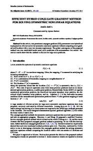
τ Figure 1. Comparison of the performance of MHCG and NDCG methods (in term of CPU time)

τ Figure 2. Comparison of the performance of MHCG and NDCG methods (in term of number of iterations)

Table 1 lists the numerical results, where Iter and Time stand for the total number of all iterations and the CPU time in seconds, respectively. ||Fk|| is the norm of the residual at the stopping point. One can see that MHCG solves most of the problems successfully while NDCG failed to solve more than 31 test problems, and this is a clear indication that MHCG is more efficient than NDCG compared to the number of iterations and CPU time respectively. Furthermore, on the average, our ||F(xk)|| is very small, which signifies that the solution obtained is a better approximation of the exact solution compared to the NDCG. However, from Figures 1 and 2 one can easily see that our claim is justified i.e. less number of iteration and CPU time to converge to approximate solution. It is important to mention that in this paper βkH∗ is obtained using the convex combination of βkFR and βkPRP, which is quite different from our method (waziri and Sabi’u (2015)), where βk was obtained by combining Birgin and Mart´inez direction with classical Newton direction. However, in this research we proposed a hybridization parameter σk ∈ [0, 1] (24), which will guarantee a good convex combination as suggested by(Andrei (2008).

5. Conclusion In this paper, we developed effective hybrid conjugate gradient methods based on Andrei’s

AAM: Intern. J., Vol. 12, Issue 2 (December 2017)

1055

approach of hybridizing CG parameters using well-known convex combination as in (Andrei (2008), Andrei (2008)). A new convex parameter was proposed using the proposed direction in this paper and the famous Newton direction. A modified secant equation was used in obtaining the hybridization parameter together with the nonnegative restriction of the conjugate gradient parameter as suggested by (Kafaki and Ghanbari (2012)). The proposed method has less number of iterations and CPU time compared to the existing algorithms. In addition, the interesting aspect of method is that, the method is a fully derivative-free iterative procedure with global convergence property under some reasonable conditions. Numerical comparisons using a set of large-scale test problems show that the proposed method is very promising. However, to extend the method to general smooth and non-smooth nonlinear equations will be our further research.

REFERENCES Andrei, N. (2008). Another hybrid conjugate gradient algorithm for unconstrained optimization, Numerical Algorithms, Vol. 47, No. 2, pp. 143-156. Babaie-Kafaki, S., and Ghanbari, R. (2014). Two hybrid nonlinear conjugate gradient methods based on a modified secant equation, Optimization, Vol. 63, No. 7, pp. 1027-1042. Cheng, W., and Chen, Z. (2013). Nonmonotone spectral method for large-scale symmetric nonlinear equations, Numerical Algorithms, Vol. 62, No. 1, pp. 149-162. Gu, G. Z., Li, D. H., Qi, L., and Zhou, S. Z. (2002). Descent directions of quasi-Newton methods for symmetric nonlinear equations, SIAM Journal on Numerical Analysis, Vol.40, No. 5, pp. 1763-1774. Hager, W. W., and Zhang, H. (2005). A new conjugate gradient method with guaranteed descent and an efficient line search, SIAM Journal on optimization, Vol. 16, No. 1, pp. 170-192. La Cruz, W., Martínez, J., and Raydan, M. (2006). Spectral residual method without gradient information for solving large-scale nonlinear systems of equations, Mathematics of Computation, Vol. 75, No. 255, pp. 1429-1448. Li, D., and Fukushima, M. (1999). A Globally and Super linearly Convergent Gauss--Newton-Based BFGS Method for Symmetric Nonlinear Equations, SIAM Journal on Numerical Analysis, Vol. 37, No. 1, pp. 152-172. Li, D. H., wang Wang, X. L. (2011). A modified Fletcher-Reeves-type derivative-free method for symmetric nonlinear equations, Numerical Algebra Control Optimization, Vol. 1, No. 1, pp. 71-82. Liu, H., Yao, Y., Qian, X., and Wang, H. (2016). Some nonlinear conjugate gradient methods based on spectral scaling secant equations, Computational and Applied Mathematics, Vol. 35, No. 2, pp. 639-651. Ortega, J. M., and Rheinboldt, W. C. (2000). Iterative solution of nonlinear equations in several variables. Society for Industrial and Applied Mathematics. Powell, M. J. (1984). Nonconvex minimization calculations and the conjugate gradient method, Numerical analysis, Vol. 1066, No. 1, pp. 122-141. Springer, Berlin, Heidelberg. Romero-Cadava,l E. Spagnuolo, G. Garcia, F.L. Ramos, P.C.A. Suntio, T. and Xiao, W.M. (2013). Grip-connected phovoltaic generation plant components operation, IEEE Industrial electronic magazine, Vol. 7, No. 3, pp. 6-20. Sabi'u, J. (2017). Effective Algorithm for Solving Symmetric Nonlinear Equations, Journal of

1056

Jamilu Sabi’u and Mohammed Yusuf Waziri

Contemporary Applied Mathematics, Vol. 7, No. 1, pp. 157-164. Sabi’u, J. and Sanusi, U. (2016). An efficient new conjugate gradient approach for solving symmetric nonlinear equations, Asian Journal of Mathematics and Computer Research Vol.12, No.1, pp.34-43. Waziri, M. Y., and Sabi'u, J. (2016). An alternative conjugate gradient approach for large-scale symmetric nonlinear equations, Journal of Mathematical and Computational Science, Vol. 6, No. 5, p. 855. Waziri, M. Y., and Sabi’u, J. (2015). A derivative-free conjugate gradient method and its global convergence for solving symmetric nonlinear equations, International Journal of Mathematics and Mathematical Sciences, Vol. 2015. Xiao, Y., Wu, C., and Wu, S. Y. (2015). Norm descent conjugate gradient methods for solving symmetric nonlinear equations, Journal of Global Optimization, Vol. 62, No. 4, pp. 751-762. Yuan, G., Lu, X., and Wei, Z. (2009). BFGS trust-region method for symmetric nonlinear equations, Journal of Computational and Applied Mathematics, Vol. 230, No. 1, pp. 44-58. Zhang, L., Zhou, W., and Li, D. (2006). Global convergence of a modified Fletcher–Reeves conjugate gradient method with Armijo-type line search, Numerische Mathematik, Vol. 104, No. 4, pp. 561-572. Zhang, L., Zhou, W., and Li, D. H. (2006). A descent modified Polak–Ribière–Polyak conjugate gradient method and its global convergence, IMA Journal of Numerical Analysis, Vol. 26, No. 4, pp. 629-640. Zhou, W., and Shen, D. (2015). Convergence properties of an iterative method for solving symmetric non-linear equations, Journal of Optimization Theory and Applications, Vol. 164, No. 1, pp. 277-289. Zhou, W., and Shen, D. (2014). An inexact PRP conjugate gradient method for symmetric nonlinear equations. Numerical Functional Analysis and Optimization, 35(3), 370-388.