condensate ( ~u u) and four-fermion condensate. (~u~tp~) are calculated simultaneously in the Gross-. Neveu model up to next-to-the-leading order in 1/N.
Z. Phys. C Particles and Fields 47, 565 575 (1990)
ze~sch~ ~r Phys~kC P a r t i d e s
and F-ekls
9 Springer-Verlag 1990
Effective potential for local composite operators and the problem of factorization of multi-field condensates* Hong-Jian He 1 and Yu-Ping Kuang 1'2 J Department of Physics, Tsinghua University, Beijing 100084, People's Republic of China 2 CCAST (World Laboratory), P.O. Box 8730, and Institute of Theoretical Physics, Academia Sinica, Beijing 100080, People's Republic of China Received 23 August 1989; in revised form 23 January 1990
Abstract. A n e w formulation of effective potential for
local composite operators is given. The two-fermion condensate ( ~u ~u) and four-fermion condensate ( ~ u ~ t p ~ ) are calculated simultaneously in the G r o s s Neveu model up to next-to-the-leading order in 1/N expansion. It is shown that factorization ( ~ q ~ , ~ u ) = C t ( ~ ' ~ ) 2 holds only in the N ~ limit and the non-factorized part of ( ~ u ~ ) contributed by the order-1/N terms is comparable to C t ( ~ u ) 2 when taking N = 3.
I Introduction
Study of vacuum condensation is one of the important subjects in quantum field theories. In quantum chromodynamics (QCD), it is believed that at least the two-quark condensate ( ~ u ) is formed dynamically which breaks the chiral symmetry and leads to the lightness of the low lying 0- mesons. The QCD sum rule approach to hadron physics concerns even higher condensates like ( ~ F ~U~'F 7~) [1]. The basic idea of the theoretical side of QCD sum rule is to consider a vacuum expectation value (VEV) of two local operators and apply the operator product expansion (OPE) to this VEV. For example, in the study of the sum rule for mesons, the VEV of the product of two current operators (Tja(x)j~(O)) is considered and the O P E gives
i~ d4x eiqx (TjA(x)jB(O)) = ~ Ca,~(q) ( 0 , ) ,
(1)
n
where C,A B (q), s are Wilson coefficients which are supposed to be perturbatively calculable and ( O , ) ' s are vacuum condensates of various dimensions which reflect the nonperturbative aspect of QCD. The validity of such an OPE has been checked by Novikov et al. [2] with some simple models in field theory. In practical applications
* Work supported by the National Natural Science Foundation of China
of the QCD sum rule, on the RHS of (1), only the Wilson coefficients cAB(q)'s are calculated theoretically while the vacuum condensates ( O , ) ' s are left as free parameters determined by experimental inputs. In order to reduce the number of free parameters, people often make a simple factorization hypothesis ( ~ r ~ v ~ r W) ~ C r ( ~,W)2,
(2)
where C r is a constant depending on the structure of F and can be easily calculated [1]. However, application of QCD sum rule to the baryon system shows that the simple assumption (2) i s n o t quite adequate and phenomenologically the C r ( ~ ) 2 term should be enlarged by a factor K ~ 3.6 [3]. Similar conclusions have been obtained from the analysis of the p-meson sum rule with the e+e - ~ I = 1 hadron data [4] and a refined study of the pseudoscalar meson sum rule [5]. Furthermore, a careful calculation of the anomalous dimensions of the four-quark operators shows that the deviation from (2) varies significantly with the change of the renormalization scale, i.e. even if (2) is good at a certain low energy scale it may fail at some higher energy scale [6]. In view of all these, a careful nonperturbative study of the non-factorized part of the four-quark condensate, ( ~'F' ~utPF ~)Nv, seems to be important. The purpose of this paper is to develop a nonperturbative method for calculating multi-field condensates. Once the ratio between ( ~ F ~ u ~ F ~ ) N v and C r ( t P ~ ) 2 is calculated theoretically, the actual magnitude of the deviation from (2) can be precisely known, and the contribution of the four-quark condensates to (1) can be well taken into account without increasing the number of free parameters. Other assumptions in the Q C D sum rule approach may then be better tested. Calculation of multi-quark condensates in fourdimensional Q C D is rather difficult. To get some information about this problem, we study, in this paper, the multi-fermion condensates through a simple twodimensional field-theoretical model - G r o s s - N e v e u model [7]. It is well-known that there are many resemblances between Gross-Neveu model and fourdimensional QCD, namely renormalizability, asymptotic freedom and an internal symmetry U(N) related to the
566
fundamental interacton. The number of fermion components N in the Gross-Neveu model corresponds to the number of colour Nc in QCD. The nonperturbative calculation of multi-fermion condensates in the GrossNeveu model is feasible though not trivial. To study the above problem, we shall have to calculate the effective potential as a function of the classical fields of both the composite operators ~' ~ a n d ~ T ~ . It can be seen that in this case the conventional auxiliary field method for evaluating effective potential will not simplify the calculation but make the calculation rather complicated. In a previous paper [81, we developed a systematic method for directly evaluating effective potential for local composite operators without introducing auxiliary fields. This method is more convenient for doing the desired calculation. The formulation in [8] is suitable for calculating effective potential in large-N limit for theories with quadrilinear interactions or higher interactions with even number of fields. The study of non-factorized part of ( T T T T ) requires a calculation beyond large-N limit. In Sect. II of this paper, we give a new formulation of the effective action for local composite operators. This new formulation coincides with the two-particle irreducible (2PI) formulation given in [8] in the N ~ oo limit, but is convenient for doing calculation to any order in 1IN expansion. In Sect. III, we apply the new formulation to the Gross Neveu model to calculate (~,~u) up to next-to-the-leading order in 1/N expansion. The result coincides with the published ones obtained from the auxiliary field formulation [9__11]. A simultaneous calculation of ( t P T ) and ( ~ t P ~ F ) is given in Sect. IV. The result shows that factorization ( ~ q , t / , t / , ) = Ci ( @l/J)2 holds only in N ~ oo limit and the order-1/N terms contribute a non-factorized part ( q'q'q'q' )NF' The ratio ( y'T~uy')NF/CI ( TY')2 is calculated at this level and the result depends on the value of N and the renormalization scale. When we take N = 3, it is shown that ( T t P T T ) / C z ( ~1/./)2 may vary from 10 -1 to 10 ~ for a certain range of the renormalization scale, i.e. ( T ~ t / - ' ) u r is comparable to C z ( ~ ) 2. This shows the evident deviation from (2) in the Gross-Neveu model and implies the possibility of accounting for the enhancement factor ~ ,~ 3.6 by ( ~FTJTF~P )NV.
where the action S is
S[ 5F, ~u;I, L K] = ~dDx{s 7u, ~) + -[tp + ~uI + gK T~F+ P(K)}.
Here a pure source term P(K) is included in order to satisfy the consistency condition requiring that no condensate effect occurs at the classical level [12]. The importance of the P(K) term has also been shown in [8]. The classical fields 4,(x), t~(x) and 2: (x) of the operators ~U(x), ~(x) and g ~(x)~(x) are defined by 3W
3W
3-i-= 4,'
31-
~W
r
6K=g64, + Z'
(4)
where 2: is the connected part of the classical field of g T(X)~(X) and its value at I, I, K = 0 gives the VEV of g ~(x) ~(x). We can shift the spinor fields by their classical fields,
q,~4,+ q,, ~,~4,+ q,, and define
S[~, T, 4,,4,;I,I,K]-S[4, + ' t , 6 + q';I, LK] - S[4,, 4,; I, I, K].
(5)
Then the generating functional W[I, I, K] can be written as
W[I, L K] = Wo[I,-[, K] + WL[I, 1, K]
(6a)
where
Wo[1, L K ] = S[4,, 4,; I, I, K ]
(6b)
WL[I, 1, K] = -- i ln S [d T ] [ d cF] exp iS[ 7~, ~, 4,, 4,; I, I, K]. (6c) Evidently Wo is the tree level part of W and WL is contributed by loop diagrams. A partial Legendre transformation of W is given by
[8] FP[4,, 6, K] = W[I, I, K] - ~d~ --- FOP[4,, 6, K] +
Fp
+ 61) - K] L[4,, 4,,
(7)
where
ro~[4,, 6, K] = S[4,, 6, 0, 0, K] = ~dOx{s
6) + gK64, + P(K)} is the tree level piece of F p and II Partially two-particle irreducible formulation of the effective action
(3b)
F p
- - K] L[4,, 4',
~
--
(8)
iln~[dY"][dT]expiS[T, ~', 4', 6; K] (9a)
with As in [8], we consider a D-dimensional spinor field theory and study the formulation of the effective action for local composite operator g CP(x)T(x) where g is the coupling constant (g2Cp(x)~(x)~(x)~(x) will be considered as well in Sect. IV). Let ~ ( t/,, ~,) be the Lagrangian density of the spinor field,/_-(x), l(x) and K(x) the external sources coupling to tP(x), T(x) and g ~(x) T(x), respectively. The generating functional for Green's functions is
Z[I, I, K] = exp iW[I, L K] = S [d ~] [d T] 9expiS[~u, ~;I, LK]
(3a)
~[tp, t~, 4', 6;K ] = ~[~u, @,~b,6,0,0, K]
36 ]
(9b)
is contributed by loop diagrams [81. It is easy to see that
3F P
64,
3F P - I,
36
-
I
3F e 6W - g64, + 2:. 3 K - 3K
(10a) (10b)
567
Conventionally the propagator ~ is defined by [ 13] 62S i ~ - '(x, y; O, ~b, K) = 6 ~ ( y)6 ~ (x) ~e,~'=o
(11)
and the interaction Lagrangian density L~1(~, ~, 0, ~) is defined by the part in L,e(0 + ~/',tp+ ~ ) + gK(O + ~ ) 9( 0 + ~ ) besides the bilinear term ~ d O y ~ ( x ) i ~ -1 .(x, y;t~,~k,K)~(y) and terms linear in ~ and ~. In this notation [8], S[ ~g, ~, 0, ~, K] = ~ d ~ 1 7 6 @ ( x ) i ~ - ~(x, y; 0, ~, K) 7~(y) + ~dOx~e1( tp, ~, 0, t~). (12)
(a)
(b)
(e)
F P = F ~ - i Tr In G - 1 _ i Tr ( H G ) - i(0l T e x p i ~ d ~
(14)
where F ~ is given in (8) and the last term means the sum of all contributions by 2PI vacuum diagrams with propagator G and vertices determined by ~ t . The sum of the last three terms in (14) is F [ . For theories with quadrilinear or higher interactions with even number of fields, in the N--* oo limit, the proper self-energy /7 is independent of the external momentum. For instance, in the G r o s s - N e v e u model [8] H = - igA where A is defined by
,4_
ae[ 6K
(15)
- g T r G.
(16)
Thus (16) provides an equation for ,4 which is algebraic when the sources are taking to be constants and is not difficult to solve. ,4 is related to K and 22 by (10b) which is d dK
(f)
Fig. l a-g. Classification
(g)
of proper
self-energy
Q 0 0
(a)
(13)
where H is the proper self-energy of the ~u field. In [8] we developed a 2PI formulation of F e which is
(d)
diagrams
in
Gross Neveu model. The heavy line stands for the physical propagator G and the vertex is taken to be the bare vertex 89 The bars at the vertices indicate that two-fermion lines on the same side are paired
The physical propagator G is related to the propagator ~ through the Dyson-Schwinger equation G *=~-I-H,
(e)
(b)
(c)
(d)
Fig. 2a-d. Classification of proper self-energy diagrams in 2-dimensional scalar field theory with ~6 interaction. The heavy line stands for the physical propagator G and the vertex is taken to be the bare vertex ((g4/6)(CI),cl),)(q)bCl)b)(cl)ccl)c)).The bars at the vertices indicate the pairing of the fields We classify the Feynman diagrams of the proper self-energy in the way that all diagrams are composed of physical propagators and bare vertices. Examples are given in Fig. 1 (Gross-Neveu model) and Fig. 2 (2-dimensional scalar field theory with ~ 6 interaction). Different diagrams are labeled arbitrarily by an index j = 1, 2 .... and the contribution of the j-th diagram with proper multiplicity is denoted by/7j, i.e. H = ~ Hj. In j=l
the field-theoretical models mentioned above, there are always some special H~s which are independent of the external momentum, e.g. diagrams (a) and (b) in Figs. 1 and 2. Let H s be one of those H'js or a sum of such H'js and /7s - 1 7 - / 7 s .
(19)
We define a new propagator G s by P(K) = ~, + ,4.
(17)
From this we can solve K as a function of 2;, 0 and t~ and the further Legendre tranformation F[O,~,X]=
FP[O, dj, K ] -
Id~
+ X)
(18)
can be performed to obtain the effective action F(~, ~, 22). When we go beyond the N ~ o o limit, the proper self-energy/7 will be external m o m e n t u m dependent and the simple relation (15) will no longer hold. In this case we can only solve G from the Dyson-Schwinger equation and obtain A from (16). The Dyson-Schwinger equation (13) in this case will be an untractable nonlinear integral equation and thus we shall have the same difficulty as that in the bilocal operator formulation [14]. In order to avoid this difficulty, we propose, in this section, a different formulation which is suitable for calculating effective potential to any order of 1/N expansion for theories mentioned above. First of all, we give some definitions which are needed in the derivation of the new formulation.
aft I = ~ - 1 _ Hs.
(20)
Evidently, it is related to the physical propagator G by G -1 = Gs 1 - U s
(21a)
or
G = Gs + G s H s r G s
(21b)
where Hsr -
Hs - H s + HsGsH' s +.... 1 - G s H 's
(21c)
Diagramatically, G and G s are denoted by a heavy line and a shaded line, respectively. A shaded bubble inserted to a shaded line means the inclusion of the complete H s corrections to G s. The diagram for the relation (21b) is shown in Fig. 3. F r o m now on, we will talk about diagrams with propagator Gs rather than G. We will express the above mentioned Feynman diagrams in terms of Gs through the relation (21b), i.e. every heavy line in the diagram is
568 coordinate. Since K appears only in Gs, we can regard, equivalently, F [ as a functional of ~,, tp and Gs, i.e.
............ + @ + ~ + . . .
F~ - K] =- ~,1" LEO, ~P, 1.[0, ~, Gs].
Fig. 3. Diagram for the relation (21b). The heavy line and the shaded line stand for G and Gs, respectively. The shaded bubble means the inclusion of the complete H} corrections.
(24)
Then we have from (9a) and (23) - / ' , - 1 1 r d I/J] r d ~13 i././!~ exp i S
6ff'P
6Gs
S [d ~ ] [d ~ ] exp iS
~
_
o
_ iS [d ~ ] [d Ep] (~Fis/SGs) ~cp exp iN S [d tP][d cp] exp iS (a)
(b)
(e)
= iGstGGs 1 - i6HSTrG 6Gs
Fig. 4a-c. Examples of P2PR(Hs) and P2PI(Ils) vacuum diagrams
= iG s 1 + i H s r _ i 5Hs Tr G 6Gs [ - i Tr In iG s i _ ills Tr G]
-
aGs
Fig. 5. Illustration of the fact that when the bubble in e is replaced by Fls, the diagram contains P2PR(IIs) pieces to be replaced by a sum of a series of diagrams shown in Fig. 3. An original single diagram H j is now a sum of a series of infinite diagrams. We denote this summation by
Hj[G(Gs)]=
~ II~)[Gs],
(22)
n=0
where H}m[Gs] is just the contribution of the diagram of H j with all G's replaced by Gss, and H}I)[Gs], Fl}Z)[Gs] .... are contributions of diagrams with various H s insertions. A vacuum diagram is said to be partially two-particle reducible with respect to I-Is (P2PR(Hs)) if it can be separated into two diagrams by cutting two G s propagators and at least one of the two separated diagrams belongs to Hs. If a vacuum diagram is not P2PR (Fls), it is said to be partially two-particle irreducible with respect to H s (P2PI(Ils)). A P2PR(Hs) vacuum diagram must have the structure of Fig. 4a in which at least one of the bubbles A and B belongs to Hs. A P2PI(Hs) vacuum diagram may also have the structure of Fig. 4a provided none of the bubbles A and B belongs to H s. P2PI (FIs) vacuum diagrams may have other structures, for example, Fig. 4b and c. It should be noted that the bubble in Fig. 4c must be I/(so) rather than Hs since if the bubble is I I s which has a physical propagator G shown in Fig. 3, we can always cut the two shaded lines attached to the shaded bubble to separate the vacuum diagram into a shaded bubble and a diagram belonging to IIs, so that such a vacuum diagram contains P2PR(IIs) parts as is shown in Fig. 5. Having all these definitions, we are ready to derive our new formulation of F e. In terms of Gs, the action (12) can be written as
S[ tP, ~, O, ~, K] = S d~176 CP(x)iGs 1(x, Y; O, ~, K) (P(y) + SdOx{oLf,(tt*, up, ~9,~) + iqJFIsV}. (23) Note that we have chosen I-Is to be those proper self-energy terms which depend on only one space-time
6Tr G + i l l s - - - - + iHsr. 6Gs
(25)
For a field-theoretical model having interactions which include a vertex with 2m fermionic fields and the coupling constant gg(m- 1) (m = 2 in G r o s s - N e v e u model), we can choose our H s such that it has the following structure (cf. diagrams (a) and (b) in Fig. 1)
H s = i( - )"- 1mgm-1 C A " - a,
(26)
where A = g T r G (cf. (16)), C is a model dependent coefficient which can be easily claculated, and we have written the multiplicity m of such diagrams explicitly in (26). The generalization of (26) to bosonic field theories is trivial, We then define --p
FL1 -- -- i T r l n iG s 1 _ iHs T r G + I dDx(-- )mgm- 2c,d m (27a) and ~p
~
EL2 ----F [ -
~p
(27b)
FL1 9
It is easy to see from (25), (26) and (27) t h a t ff'LP2satisfies
a,r~2 6Gs
iHsr.
(28) ~p
Equation (28)~determines the content of FL2. First we note that if /~LP2 contains P2PR(Hs) diagrams (cf. Fig. 4a), contain terms like AGsHs which 9 must ! Up do not belong to tHsr. Therefore, (28) implies that F m is not contributed by P2PR(Hs) diagrams. There are two kinds of P2PI(Hs) diagrams. The first kind is the type of Fig. 4c, the functional derivative a/aGs of it includes 9 t ~p iH(s~ which is also not in r Hence /-'L2 is not contributed by this kind of diagram either9 The second kind includes all other types of P2PI (Hs) diagrams (e.g. Fig. 4a with A, B not in H s, Fig. 4h etc.), the functional derivative 6/6G s of which belongs to H'sr. Thus (28) tells Up that F m is contributed by all P2P1 (I-Is) diagrams of the second kind. There are two kinds of interactions in (23), namely the interactions in 5a~ and an extra interaction
a?'L/a s
569
i ~ H s ~.. Vacuum diagrams including the latter vertex will certainly contain a factor of H s attached with two Gs legs, and evidently they are not P2PI (Hs) diagrams of the second kind. Therefore the second kind P2PI (Hs) ~p diagrams contributing to F m are all composed of propagators Gss and vertices determined by Lr The fact that /~[ 2 contains all the second kind P2PI (/Ts) diagrams is easy to understand since the use of Gs instead of ~ (H s insertion) can reduce some P2PR (Hs) diagrams but does not affect P2P1 (Hs) diagrams and our F ~ (cf. (27a)) contains the P2P1 (Hs) diagram of the first kind, ~p so that F m must contain the contributions of the rest P2PI (Hs) diagrams. A careful counting of the multiplicities of the P2PI (Hs) vacuum diagrams and the self-energy diagrams in HsT checks that the above conclusion is correct. An up to 4-loop check is given in the Appendix. Our new formulation of Fe[~b, ~ff,K] is then ~) + g K ~ + P(K)} -- i Tr In iGs i _ ~dOx(_)m(m_ 1)gin- 2CA~
III Calculation of ( g ~'W) in Gross-Neveu model to next-to-the-leading order in 1 I N expansion
In the Gross-Neveu model, the action S[ ~u, ~, K] is [12]
S[ iF, 7p, K]
= SdZx
{ 7Pi#~
+
89
..]_gK ~tF + P(K)}
I~r
(31) in which the pure source term P(K) determined by the consistency condition is [12]
P(K)-- I~K
(32)
Equation (17) is then K = Z' + A.
(33)
For simplicity, we ignore the external sources ]-and I and the classical fields ~k and ~ in the calculation since eventually ( ~P ) and ( ~ ' ) vanish. Then the interaction Lagrangian is simply
Fe[~, ~, K] = ~d~
5a,(~', ~ ) = 89
~'o)(q~b %) -
~(
(29)
(34)
where the last term means the sum of all P2PI (Hs) vacuum diagrams with propagator Gs and vertices determined by 5at except the type of Fig. 4c, and we have rearranged the terms in T ' ~ (27a) by using (16) and (26). Now the unknown part in Gs is just the external momentum independent quantity 1-Is or equivalently A (cf. (26)), and (16) which determines A is algebraic. Therefore (29) can be used to calculate FP[~, ~, K] to any. order in 1/N expansion without being confronted with the difficulty of solving nonlinear integral equation. The main procedure of calculating the effective potential is summarized as follows.
where 2 = gZN is supposed to be finite when N ~ m. Now we take our 11s to be H1, the contribution of Fig. la, i.e.
- i(0lexp i~dnxsallO)'e2e1(ns),
i) Calculate the RHS of (29) to the desired order in 1/N expansion to get Fv[~k,~,K] which contains an unknown quantity A. ii) Solve (16) to get A. iii) Solve (17) to get K = K[~k, if, X]. iv) Make the Legendre transformation (18) to get the effective action F[~k, tff,X] from which the effective potential is obtained. The formulation can even be generalized to the case that H s is arbitrarily chosen. Now the bubble/-/~s~ in Fig. 4c should be replaced by a generalized quantity H , which is defined as the contributions of the /7s diagrams in which all those propagators connecting both external legs are replaced by Gss ~while other propagators are kept to p be G's. In this case, F m is contributed by all P2PI (1I*) diagrams except the type of Fig. 4c with 11~s~ replaced ~p b y / 7 * provided that FL~ is taken to be ~p
FL1 = -- iTrlniGs 1 + A[Gs]
FIs =/7~ = - igA.
(35)
Comparing (35) with the general form (26) we see that m = 2 and C = 1/2 in the present case. The propagator Gs is now determined by
iGs
1=
i~ + gK -- gA = i~ + g~,.
(36)
In the N--* 0o limit,/7s coincides w i t h / 7 (cf. 05) and (35)) and Gs = G (cf. (13) and (20)), so that the present P2PI (/7s) formulation reduces to the 2PI formulation in [8]. Now (29) is
FP[K]
= a~d2x[K2
-
A 2] - i Tr In (i~ + g2~)
-- i(01 ex p i~d2x5a, [0 )P2PI(
(37)
FIs)"
Up to next-to-the-leading order in 1/N expansion, the last term in (37) is contributed by P2PI (Hs) diagrams shown in Fig. 6 where the multiplicities of the diagrams are not explicitly shown. The calculation is elementary and the result is
1-'e[K] = ' d2x{ ; K2 - 21-d2 -1n'S2(lng2"S" z~-- 1) A -~dk21n+ [l~n-l(g2~2+ '8~z QnlQ+}ol):
~T-
_
, 8a,
(30a)
and A[Gs] satisfies (a)
6A fiGs
6Hs Tr G. i ~Gs
(30b)
(b)
Fig. 6a, b. P2PI(Hs) vacuum diagrams contributing to the last term in (37)
570
where
Q=
~/
42X2
(38b)
1 + Nk 2 ,
and A is a momentum cut-off introduced for regularizing the divergent integrals. The last term in the curly bracket is of order-1/N which can be seen from the relation 82,a~2 QdQ dk 2 -S (Q2_ 1)2 Note that except for the first two terms, all other terms in (38a) have the feature that they depend on K through 27[K]. The Legendre transformation (18) can then be performed very easily by simply using (33) without solving A from (16) and we get
F[X] = jd2x{ -1- 222 - :rc222(lng2 ~ 5~- 2 ]~dk2ln[1 + 2 (lng27 2
l n Q + 1"]]~
+ 0(1~).
(39)
The effective potential is thus Veffr,~"] = -- F[27]/~dZx = ~,272 + A2dk 2
[
, ~ /,
+ !8,1n 9
471
g2~'2
2
+
272 In
.2
(41a)
where o
U = Uq + U~ + U I
(42a) k2
Uq-aj~dk21nVl + ~ l n g ~ + ~ 2 L
in(1 +
2 //
k2
g2.2~
jj..
(42b)
+l -1 g2~2"~
l+ (ln 2.2+ k2 )
A2 2
In. 2+Qln
(1 + #2 + ~1n222"] "] ~--2ff-(1 2/t , 2 ] ]
A2
(4 d,
The term Uq is just the constant quadratically divergent term which can be dropped. U~ is the logarithmically divergent term and UI is the finite part. In our renormalization scheme we put A = g . in Uz which makes Ut = 0. Therefore only Uf contributes to Veff and thus our finite Vaf is Vaf=~
2 2// z~2
+ 4 n S ~ln #2 - 1
) /
2dk21nl+ In + Q l n _+1 + lim i 8~ #2 g2#2~ A~ 2 /" k 2 1 + ~ l n 95~2 + A2 92222 [ In 9z#z _ _+ ( 1+ " 2 - 2 ~ ( 1 "+ Z~ln $ 2 ) ) 4n ~'2 2 \ 2x ~2 A2
Let us introduce subscripts 0 and 1 to denote, respectively, quantities of leading order and next-to-theleading order in 1/N expansion. In the N ~ oo limit the last term in (43) vanishes and the first two terms lead to the extrema
22o(O)={o..e-~/a ,
(44a) (44b)
It is easy to see that the nonvanishing solution (44a) is the true minimum of Vaf. (44) differs from the result in [7,8] by a finite renormalization due to the different renormalization schemes. When we take into account the last term in (43) (order-l/N correction), the extremum condition is 2,
222(0) +
dVff =22(0) 1 + dX z = z(o) 21r m ~
Next we separate U into
o 8~
(42c)
1+
4~ ~1n9~5+
(41b)
7
2 //
g2272/
Q-{" 1 ~ ]
U - f d k 2 1 n [ 1+ 2 (in 272 + Q in Q + 1"]]
A 2 \~
A2dk21n U f - t i m ! 8~
32 +01nQ i/j"
- 1 + U.
2
+ 2~lng2~5)J
;
(40) This is just the formula given in [9, 10] with the auxiliary field a replaced here by the classical field I2. The last term in (40) contains quadratic divergence. However, it is easy to see that the term proportional to A 2 is merely a constant (independent of 27) and thus can be ignored. The 27 dependent part contains only logarithmically divergent terms and finite terms. Let , be a finite scale parameter. We shall take a renormalization scheme in which we put A--* oo in the finite terms and replace A by g , in the logarithmically divergent terms. It is easy to check that this scheme is equivalent to the modified minimal subtraction scheme (MS scheme) in dimensional regularization. We first replace the A's in the explicit logarithms in (40) by g,. This corresponds to doing MS renormalization for the l-loop diagram and all the subdiagrams in Fig. 6b. Then (40) becomes =
9ln(1
1 z~ 2
// g2272_ 1"~ ZZ~ln ~_2-
2:(1 +
02222[- A 2 ( .2 U,- ~[1n92.2 + l+z~-
xN J
where
2rt x/
l +/'i~i~g(O)/NA2) Q2 _
=
1
0
(45a)
571
classical fields Z and ~ are defined by
lnQ+ 1 Q-1
6W
l + ;n(ln~+QlnQ+ 1[A In ~292# 2
l)Q-I
~ ( 1 + ~--ln S:(O)) 2n I~2 ]
2
2~
A2
(45b)
Thus the solution is
6W
-- z~ 2 ~- ,--,~.
(53)
6K4
where • is the connected part of the classical field of g2~U~u~u. The relation between ~, S 2 and the non-factorized part (g2~UkU~uTJ)NF can be seen as follows. We know that the factorized part of (92 T ~ u ~ > is (g2 ~.ttl.t~.t~.t)F = C l ( g 2 ~tlct )2 = C I S 2(0).
In the Gross-Neveu model, C I = 1 - 1 / ( 2 N ) . non-factorized part (g2 g.,~uT~U>Nv is then
2:(0) = So(0 ) + X~(0)
The
(g2 tI.t~/zt/* )/VF = (g2 t/_tt/.lt/*~Cr~ __ (g2 t/It/zl/*~ ) v
(46a)
={ +#e-~/z(1-~))+O(N~2)0.
(46b) For the true minimum (44a), 7(0) reduces to ~(o)=
-- z~7,
~K 2
dQ ~/1+(402#2/A2) e-2~/'~Q(Q2- 1)
1
A2
n
21ng2/~ 2 -- 2
= ~(0) + (1 - C,)S 2(0).
To determine the pure source term P(K2,K4), we examine the Euler Lagrange equation in the case of constant sources ~cEg(~c ~c) + K2 +
In2.
(54)
2K4g( ~ ~uc)] = 0.
(55a)
Its nontrivial classical solution is
(47) g( ~'~ ~/'c)=
So that the VEV of g ~'T is
(gTT>=S(O,: ++_#e-'~/Z[l-1 ( 2 - In 2 ) ] + 0 ( ~ 2 ) . (48) This coincides with result in [11]. Finally we point out that (45) can also be derived in a different way. When we take K = 0, (33) gives a relation between the extremum qualities Z'(O) = - A(0).
(49)
So that (16), when K = 0, gives an algebraic equation for X(0), i.e.
S(O) =(6F~']
\ 6K ]K=O
=-gTr(Gs+Gfl'srGs)lx
o.
=
(50)
It can be seen from (27a), (28) and (33) that (50) is exactly (45) as it should be. Therefore 2:(0) can actually be obtained by solving (50) without knowing the explicit formula (43) for Vaf(S ).
K2 1 + 2K 4"
(55b)
and from which we get the classical value of W:
Ws
K,] = S[ q'~, ~P~,K2, K,] = Id2x
2(1 + 2K,) + P(K2, K,) .
(56)
The consistency condition requiring that no condensate effect occurs at the classical level is now [12] - -
6K~KTIK2,K4=O
= 0.
(57)
This determines P(K2, K,,) -
K2 2(1 + 2K4)"
(58)
Let g2(K4) = (1 + 2K4)g 2,
(59)
Then (52) can be written as IV The problem of factorization of ( W W W W ) in G r o s s - N e v e u model
S[ 'P, cp, K2, K4] =~d2x{~i~T +gg i -2 (tptp) Z +gK2 UI*~t*+
To calculate (g T T ) and (g2 ~ u T ~ T ) simultaneously, we consider the generating functional Z[K2, K4] = exp iW[K2, K4]
=~[d~][d~]expiS[T, ~ K 2 , K 4 ] ,
(51)
where S[ T, ~', K2, K4] =
1 2( ~ T ) 2 + gK2 Cp7., ~d2x{ ~'i~ T + ~g + g2K4( CPT)2 + P(K 2, K4)}. (52)
Here we have also ignored the sources I-and I and the corresponding classical fields ~ and t~ for simplicity. The
P(K2" K 4 ) }.
(60) This looks just like the action (31) in Sect. III except that the coupling constant in 5e, is 0 rather than g. Thus (33) (36) become now
K 2 = (~/g)2(S + A),
(61)
,,~l( tt"t, ~'t) = l o2( U[latlla)( U[~btPb) -= 2"~ _ ~,)(c/' b Tb), (62) ~ ( T,
OZN, Hs = H~ = - iO(O/o)A,
where 2--
(63)
572
and
iGs t = i~ + 9(0/9)~.
(64)
Now in /'[, K 2 still appears only in Gs._Therefore F[[K 2, K4] can be equivalently regarded as F[[Gs, K 4 ] and our formulation given in Sect. II still holds. Equation (2.9) is now
FV[K2, K~] =~d2x K22
2(1 +2K4)
iTrln(i~+O(O/9)S)
-- ~ d2xt(tff/9)2 A 2 --
; (ln(0/9)'So + //2 + (~o In (~o - 1 dk 2 ~ \ U" - 2K4 fa o 8g 2 (ln(0/9)4~ ln(~O + 1)"
)z
(68c) Now U' is of the same structure as (41b) and thus it can be renormalized in the same way as we have done for (43), i.e. after renormalization the finite /J' is
/.7'
i(Olexp i ~ d 2 x ~ i l O )'e2et( ns)"
l i m ~ i ~dk2 = g ) = A-~o( o 8~
(65) Up to order-l/N, the last term is contributed by the same diagrams shown in Fig. 6 except that the coupling constant at each vertex is now 9 rather than 9. Therefore
Fe[K2'K4] = ~d2x{2(l K2+2K,) 2 (9/g)2 2A
l + 22rc(ln(O/9)4N~+ Ooln %~+ll 2 In k2 _ + 1+ ........
a~dkZ [
4f~(O/g)2z~,2
//2
9ln(1 + 2
~ (ln(O/9) ~Sz t-(~ln(~+ 3 ~ 11) 9 , (66b) //2
where
k2 J
~ln /9).~f2X~ // //
2~
2 1 +2re
-F O(\ N1~'], 2]
1+2~\
4~
2~ ( 92//2
A 2 "~
(69)
2~:In ,~u2) ]}"
(66a) - ! 8nln
(0/9)4S2
"ln
.[lngA;2 + (1 4 "(ln \ ('0/9)4Z' ; 2 1 )2- - / 7 }
+G 025_1/
The divergences in U" can be analyzed in a similar way. We can write
(70a)
--t! --r = Uq + U~ + U--tts U" K4 JA ~ Ut!
X~
(66c)
Nk 2
Here we have made the replacement A ~ 9//in the explicit logarithms in (66). Elementary calculation shows that when we drop all O(1/N 2) terms, (66) can be further written as
r,,13