Jl. of Computers in Mathematics and Science Teaching (2003) 22(3), 185-205
Effects of Computer-based Laboratory Instruction on Future Teachers’ Understanding of the Nature of Science RICHARD STEINBERG City College of New York USA
[email protected] With computer-based instruction, numerical data collection and analysis are performed effortlessly in the laboratory, simulations with idealized conditions are a click away, and abstract concepts that are difficult to visualize are represented in full-color animated displays. Many of these computer applications are designed to help students understand physics by clearly presenting the outcomes of physics or by making it easier to do scientific experiments. However, in the effort to get to the product of science, is there a danger of misrepresenting the process of science? This is a particularly important question in college science classes for future teachers where we try to model instructional practices that promote inquiry and active learning. If we want students to take responsibility for building their own understanding of science, they need to develop an understanding of what science is. In this study, we look at pre-service teacher classes in physics, one of which uses computer-based laboratories extensively. The context presented is one-dimensional motion, which is covered in the computer-based class with motion sensors interfaced to computers. We consider student performance in an interview setting and on an examination problem.
In the implementation of teacher education programs, there is a call for teachers to learn “science content through the perspectives and meth-
Steinberg
186
ods of inquiry” and to use “technological resources that expand their science knowledge” (National Research Council, 1999). With computers, science teachers have opportunities to engage students intellectually, to explore more meaningful and exciting subject matter, and to learn the technology itself. In this paper, we use student interviews to probe learning in a physics class for future teachers. The class used motion sensors as a focal point of instruction. We find that after instruction, some students do not connect their qualitative understanding of the material to the formalisms developed in class. One stated “I’m sticking with my formulas instead of my thoughts” when trying to resolve an apparent discrepancy. Other students are unable to interpret experimental data obtained with non-computer based equipment. For example, one completely changed her analysis of an experiment to account for typical measurement errors. We also look at how students in different classes (using different methods of instruction to cover the same material) performed on the same examination problem. The relationship between computer-based instruction and student performance is explored and implications for instruction are discussed. STUDENT INTERVIEWS Classroom Context Student interviews were conducted with pre-service teachers enrolled in a popular computer-based introductory physics class for future teachers. The class, Phys 115 at the University of Maryland, is intended for students interested in teaching in elementary or middle school. The goals of Phys 115 go beyond teaching subject matter. They also include helping future teachers realize that science is accessible, exciting, and relevant to students of all ages and that science involves doing and understanding, not just memorizing. Phys 115 is extremely hands-on and interactive. In the particular class studied, most of the experiments conducted were microcomputer-based laboratories (MBL). For many years MBL have been successfully implemented in college physics courses (e.g., Thornton & Sokoloff, 1990; Laws, 1991). For about five weeks in Phys 115, there was an emphasis on using motion sensors combined with graphs in teaching about motion. Before using the computers or doing the experiments, students made predictions about what they thought the graphs would look like as they moved in different ways
Effects of Computer-based Laboratory Instruction
187
in front of the sensors. After carrying out the experiments, they compared the results with their predictions and accounted for any differences. They considered multiple representations of motion including graphs and equations. In addition, students were constantly articulating their understanding in words and explaining their reasoning. Investigations of student learning in college physics courses suggest that these kinds of strategies and tools are better than traditional instruction at helping students understand physics concepts (Redish, Saul, & Steinberg, 1997; Steinberg & Oberem, 2000). Furthermore, students in Phys 115 showed strong gains with respect to attitude and affect. There is no question that the students began to appreciate the value of an interactive and collaborative science classroom. Student comments about learning science while taking Phys 115 consistently reflected significant gains in perspective on the teaching and learning of science. For example, one student noted “When I have learned science in the past it has been purely memorization for a test and then I forget it. [Phys 115] is very hands on though, so I can actually see what I am doing and understand what I am learning.” Another said “I’ve learned that interesting relevant topics and hands on learning experiences that demand thought and each person’s ideas are the most effective way to teach people science.” However, the purpose of this research was to study Phys 115 students’ understanding of the nature of science having learned extensively in an MBL environment. Protocol During the last week of the term, eight students out of the 27 enrolled in a Phys 115 class were interviewed. All were undergraduates. Seven were elementary education majors. The eighth was planning to become one. The students volunteered to participate in the interviews and tended to be doing well in the course. Five of the students received an A, two a B, and one a C. The students were interviewed one at a time and each interview lasted between 45 minutes and an hour. The interviews were videotaped and transcribed. To various extents, the students demonstrated conceptual difficulties similar to what has long been observed in traditional physics classes (Trowbridge & McDermott, 1980; Trowbridge & McDermott, 1981). Some could not distinguish velocity from acceleration. One said, “you would have to measure the velocity, which is the acceleration or the speed.” Another said, “acceleration is the speed of it and velocity, I don’t know, it’s just anoth-
188
Steinberg
er word.” Other students used meters and inches interchangeably or used flawed measurement technique. In this paper though, the focus is on difficulties students had carrying out and interpreting scientific experiments involving motion. The interview protocol consisted of two distinct tasks. The subject matter on which they were based was covered in the course. For the first task, students were shown a strip of paper containing a series of dots with times written next to them. (See Fig. 1.) The interviewer explained that the dots were created by a cart rolling in a straight line and marking the trail at the clock times indicated. After being sure that the students understood how the pattern was made, the students were asked to describe the motion of the cart and to calculate the velocity and acceleration. The interviewer always asked them to explain their reasoning and gave them every opportunity possible to come up with an answer and explanation. The main goal of the interviews was to probe student beliefs about science. Instead of asking students directly about these beliefs, students were presented with two tasks in which they had to demonstrate their scientific skills in real contexts. In this way, the focus was on inferring student beliefs from how they actually do science and not from how they think they do science.
Figure 1. Pattern of dots on strip of paper shown to students during interview. Students were told that the dots were created by a moving cart and then were asked to describe the motion of the cart. Figure 1 represents the motion of a cart slowing down as it covers less distance in successive one-second intervals. The change in displacement in successive intervals is constant so this particular motion corresponds to uniform acceleration, which is a relatively simple motion that the students had covered. While the dot representation was unfamiliar, it was hoped that the students could translate from one representation to another. Such skills are more important than facility with a given representation or tool if the students are to foster student-centered learning in their own classrooms. After finishing with the ticker tape, the interviewer asked the students to consider a completely different experiment. An actual cart rolling down a 1.5-meter ramp was shown and the students were asked for a description of the motion. After students noted that the cart was accelerating, the interviewer asked them to determine the value of the acceleration. A stopwatch, ruler, marker, and various other materials were available.
Effects of Computer-based Laboratory Instruction
189
Since the cart moved with uniform acceleration, there are several ways to determine acceleration in just a few minutes. Acceleration is the change in velocity divided by the change in time. The change in time can be determined by using the timer to measure how long the cart is on the ramp. The initial velocity is zero and the final velocity can be determined several ways. One way is to time how long the cart takes to go a measured distance after leaving the ramp, where it is moving with reasonably uniform velocity. Another way is to reason that the average velocity (the length of the ramp divided by the time on the ramp) must be half the final velocity since the acceleration is constant. In practice, these different experimental techniques yield values of acceleration within a few percent of each other and within a few percent of the expected acceleration (0.31 m/s2) for the particular angle of the ramp. Overview of Student Performance At first, the dot representation confused most of the students. Seven of the eight students initially said that the dots getting closer together indicated that the cart must have been speeding up. Jill gave a typical answer.1 “There’s a dot at each second, and it appears that the dots are becoming more frequent, so that means [the velocity] is increasing.” Three of the students who said that the cart was speeding up stuck with their answers, even as they explained their reasoning. Four of the students, including Jill, corrected themselves and were able to qualitatively analyze the experiment correctly: “In one second it went farther [at the beginning] than one second [at the end] … so it’s slowing down.” Joan was another student who started by saying that the cart that made the ticker tape was speeding up. She then calculated an acceleration of “point 179.” (She gave no units.) Joan later changed her mind, but only after being asked to think of the experiment in terms of “common sense.” Joan:
As time increases, every second the cart accelerates by point 179.
Interviewer: Okay. What does that mean? Joan:
Every second the cart would move point 179.
Interviewer: [After hesitation by Joan.] Tell me what you’re thinking, that’s what I’m really trying to figure out.
Steinberg
190
Joan:
I could do that and say, like, common sense what’s happening but I don’t know if I could figure [the acceleration] out.
Interviewer: Tell me what you’re thinking with common sense. Joan:
Common sense is ... if it is traveling less distance in one second it must be going slower. Right, and it means that more distance means it must be going faster because it’s covering more distance in one second so I was backwards [before].
The second interview task was an even greater challenge for the students. No one had a strategy that could result in a reasonable value for acceleration. Several of the students determined values that were not acceleration and a few of the students had no idea how to proceed. Many were clearly frustrated by their own confusion. After the interview, Fran stated, “I had no clue how to set it up. If I had a computer I could have set it up in 2 seconds but now that you’re doing it on your own without a computer it’s a lot harder.” Below, we describe a few of the most common scientific problems that the interviewed students demonstrated. We also try to make sense of the role of the MBL instruction in the development of the students’ ideas about science. Difficulties Integrating Qualitative Scientific Reasoning An important part of learning science involves making qualitative sense of one’s observations and building and using tools that allow for a more powerful analysis of some class of phenomena. Understanding how one’s qualitative interpretation connects to the tools is obviously critical. Throughout the semester, the students in Phys 115 had the opportunity to use a computer for data acquisition and display. Students were able to see a real time representation of their motion as they moved in different ways in front of a sensor. Graphs and concepts were thus readily accessible to the students as they moved. However, answers were coming from a black box. The students did not automatically have the opportunity to build their own answers. Instead, they seemed to rely on an authority, in this case a computer, to provide an answer.2 By the end of Phys 115, it appears that some students had not developed sufficient skills in connecting qualitative analyses to other measures of motion. In the interviews, several ended up abandoning excellent judgment in favor of something incorrect, as the following examples illustrate.
Effects of Computer-based Laboratory Instruction
191
Betsy Betsy initially said that the cart that made the ticker tape pattern shown in Figure 1 was speeding up. However, she was unsure and tried using some of the kinematic equations to help her decide. She did not know how the quantities in the equations related to the dots on the ticker tape though and became quiet and unsure. Eventually, she looked up from her equations and stated: Betsy: I’m just trying to picture this visually in my head … I was trying to think, if it’s decreasing, then it is slowing down so the drops are going to get closer and closer together …So it’s definitely decreasing in speed.
This is an excellent qualitative description. Her use of the word “visually” is significant in that she appeared to be using her intuition instead of just a classroom formalism. After realizing that the cart was decreasing in speed, Betsy tried to use equations to describe the motion in greater detail. Betsy also created a table to help her analyze the problem. For the distance entries in her table, she measured the distance of each dot from the first dot, starting with zero. For each time entry, she wrote the “seconds” value from the clock reading with each dot. Note though that the clock happened to start with the time seven seconds after the nearest minute instead of zero. Betsy later added velocity to her table. To determine the velocities at each time, Betsy divided her distance by time. This is incorrect because it considers distance and time values instead of intervals. Furthermore, it suggests that if the second’s value on the clock had been different, all of the velocities would have been different, even if the motion were identical. In addition, Betsy divided wrong in one of her velocity entries. It turns out that Betsy’s mistakes implied that the velocities were first increasing and then decreasing. She noticed that this was inconsistent with her earlier description and stated, “all of these should be decreasing.” Unfortunately, Betsy did not have much faith in her qualitative description and did not seem very disturbed by the contradiction between her “visualization” and her calculation: Interviewer: I want to go back and ask you again the beginning question. How would you describe the general motion of the cart? Betsy:
It would be increasing then decreasing speed.
Steinberg
192
Interviewer: Is that consistent with what you said before? Betsy:
No.
Interviewer: Which one is right? Betsy:
[Without hesitation] I think my last one is right because I did all of this work to prove it ... I’m sticking with my formulas instead of my thoughts.
Jane As another example, Jane abandoned an appropriate qualitative description of the cart rolling down the ramp in favor of poorly interpreted experimental data. Jane had no problem describing the motion of the cart rolling down the ramp. “It will start off slow and since it’s on an incline it will just keep going faster and faster.” She then used the timer to measure the time it took the cart to get to each of the locations A through F shown in Figure 2. By subtracting times, she determined the time the cart spent in various intervals. Knowing the lengths of the intervals, she calculated the velocity of the cart for various parts of the motion. According to her measurements, the time intervals for D-E and E-F were equal and both velocities were “33 m/s.” (She measured centimeters but called them meters.) Similarly, she determined that the velocities in intervals A-B and B-C were both “20 m/s.” Instead of recognizing the limitations in what she was able to experimentally distinguish, she decided that all of the speeding up must take place in the central region where she did not try to measure the velocity: Jane:
Well the velocity from here [A] to here [B] is constant and the velocity from here [B] to there [C] is constant. But somewhere in between here [C] and here [D] it changes because it jumps from 20 meters per second to 33.3 meters per second.
After an erroneous interpretation of her experimental results, Jane chose to no longer stay with her reasonable description that the cart was moving faster and faster as it moved down the ramp, but rather that the acceleration all took place in the middle, where she did not measure.
Effects of Computer-based Laboratory Instruction
193
Figure 2. Schematic to help interpret Jane’s reference points. Jane did not draw a diagram like this, but instead pointed to different parts of the ramp while she was speaking. Lucy Betsy and Jane both used some description or measure of motion as a reason to abandon an accurate qualitative description. Other students had faulty qualitative descriptions that they tenaciously defended despite what appear to be convincing reasons to improve their understanding of the motion. For example, Lucy began her interview by saying that the cart that made the ticker tape pattern must have been speeding up: Lucy:
I know that the cart must be going faster because the dots are getting closer together. ... It must have gone faster to get the dot closer to the starting point.
Interviewer: How does going faster make the dot get closer to the starting point? Lucy:
Because it could drop it sooner.
Despite not having the right answer, Lucy showed signs of conceptual understanding. She recognized that the speed was changing by equal amounts in equal time intervals and how that represented constant acceleration, even though she had the sign of the acceleration wrong: Lucy:
Well it looks like [the distance between the dots] is increasing by point five cm every second. ... The acceleration is point five centimeters per second squared. ... It has a constant acceleration. The velocity is changing constantly.
Nevertheless, Lucy continued to stick with her claim that the cart was speeding up in the face of very conflicting information. Interviewer: Can you tell me with a number what the velocity is at various points?
Steinberg
194
Lucy:
From here to here [between 1st pair of dots] it’s 4.5 cm per second and from there to there [between 2nd pair of dots] it’s 4 cm per second and from there to there [between 3rd pair of dots] it’s 3.5 cm per second.
Interviewer: Okay, so what is happening to velocity? Lucy:
It’s getting faster because it’s decreasing.
Even later in the interview, despite her numerical calculations and much discussion about her reasoning, Lucy continued to argue that the velocity of the cart was increasing: Interviewer: What is happening to the numbers? Lucy:
The numbers are getting smaller.
Interviewer: The numbers getting smaller means the velocity is increasing? Lucy:
[Yes.]
At the very end of the interview, the interviewer asked Lucy to describe what pattern of dots the cart rolling down the ramp would make if it dropped oil at equal time intervals. She said that the cart was speeding up so the pattern would be the same as the ticker tape shown in Figure 1. She was asked to draw the pattern of dots. She did, with the dots ending up very close together. She was asked to consider longer total times for the cart motion, guessing that she would recognize her dot spacing makes it impossible for the cart to go very far. She stuck with her prediction. The interviewer had her pretend a paperclip was the cart and had her move it along her sketch. She still did not change her mind. The interviewer finally had her act out the motion by walking and dropping paper balls. The first three times she walked and dropped she insisted that the balls were doing what she predicted. After the fourth trial, when asked to greatly exaggerate her motion, she finally changed her mind about the whole thing. Qualitative scientific reasoning and computer-based instruction When doing science, one moves back and forth between qualitative and quantitative scientific reasoning. One informs and guides the other. When a computer is the focus of instruction, such as in MBL, there is the possibility that part of this back and forth can be missing for the student and that the
Effects of Computer-based Laboratory Instruction
195
computer can be interpreted as a source of answers without the need for objective interpretation (Steinberg, 2000). Student performance during interviews suggests that Phys 115 students finished the course with many counter-productive ideas about what it means to make sense of science. For example, students did not appear bothered by gross inconsistencies in the different ways that they thought about a given experiment (Hammer, 1994b). The use of MBL in Phys 115 represents only one particular implementation of the computer. In other computer learning environments in physics, the computer has been used in a way that supports the development of student qualitative scientific reasoning skills. For example, through student programming of the computer, Papert built on the work of Piaget to define an unconventional learning environment in which the emphasis is on the intellectual development of the student (Papert, 1980). Regarding Newton’s Laws, he describes a computer “microworld” in which students, by defining and exploring the microworld, become architects of their own learning instead of passive recipients of counterintuitive laws given from authority. Studies at Berkeley have shown that MBL could be used to foster scientific reasoning skills (Friedler, Nachmias, & Butler, 1989; Friedler, Nachmias, & Linn, 1990). In developing the Constructing Physics Understanding software, Goldberg and colleagues have focused on using software to help students, typically future teachers, construct their own ideas of physical phenomena (Goldberg, 1997). Regarding representations, Phys 115 students did not choose or produce the representation; the choice was made for them. This can result in students interpreting the computer as a source of information and not as a tool for a scientist. In contrast, diSessa reported that the computer aided students in inventing their own representations (diSessa, Hammer, Sherin, & Kolpakowski, 1991). However, all the examples above are very different from the approach used in Phys 115 and most other MBL physics classes. Weaknesses Interpreting Real World Experimental Data Using the computer to perform much of the experimental work has advantages and disadvantages. An advantage is that there is time freed up for students to engage in more intellectually meaningful activities. A disadvantage is that the students might have less opportunity to interpret all aspects of a real world experiment. Several students who were interviewed had difficulties in interpreting important features in the experimental data.
Steinberg
196
Fran When doing an experiment, one normally looks objectively at the data and tries to make sense of what is happening. However, Fran used what she expected to see in the data to dictate what the data should look like. For the cart rolling down the ramp, Fran measured that the cart took 2.4 seconds to go 46 cm. She also measured how long the cart took to go 47 cm. Not surprisingly, she measured 2.4 seconds again. Without elaborating, she noted, “I think the first one is wrong.” Nevertheless, she plotted these two points and several others on a distance-time graph. She drew a straight line that appeared to go through the 47 cm point but not the 46 cm point. (If she had been more careful, she would have realized that these 2 data points were imperceptibly close to each other on her graph.) She argued that one point was better than the other because it made the graph look linear. She then argued that because the graph was linear, the cart must have moved with constant velocity. She did not recognize the circular reasoning or the obvious non-constant velocity of the cart. Fran’s confusion then played a role in her having difficulty resolving her qualitative reasoning with her graph. Before graphing the motion, she said that the cart was speeding up as it went down the ramp. After seeing that her graph implied a uniform velocity, she changed her mind: Interviewer: You point to the ramp and tell me that [the cart] is speeding up and then you point to your graph and tell me it’s constant. Fran:
Reading the graph helped me to understand it better. [My earlier prediction] was just a guess.
Interviewer: Okay, so what’s really happening now that you’ve done the graph? Fran:
It’s staying at the same speed the whole time.
Fran had difficulty interpreting her experimental data, which led her to an erroneous description of the motion. Following this difficulty, she was unable to resolve, or even recognize the discrepancy between her qualitative description and her calculated answer. Denise Denise also demonstrated weaknesses in conducting a simple experiment and interpreting the results. She timed 1.4 seconds to reach the 10inch mark. She then timed 2.1 seconds to reach the 20-inch mark, although
Effects of Computer-based Laboratory Instruction
197
this turned out to not be a very careful measurement. For the 30-inch mark, she timed 2.1 seconds again. She apparently recognized the impossibility of having the same clock time for different cart positions and started to laugh. She said, “I’ll try again” and re-timed the distance a second and a third time until she got a longer time measurement. Given that her mistake was from the 20-inch measurement, she had made matters worse while failing to understand experimentally what was happening. Real world data interpretation and computer-based instruction Elementary and middle school science teachers and their students are likely to look at a variety of science data across different subject areas in their classes. Interpreting data that deviate from ideal conditions is an important part of doing and teaching science. Several of the interviewed students, including Fran and Denise, were unable to interpret non-ideal data, even in the subject that they had just studied. In many instructional MBL experiments, classroom activities do not build the skill of making sense of real data. The computer does the data acquisition and processing. However, the computer can also be used to enhance the collection and interpretation of real world data. It can be used to change the structure of the learning environment to one that helps students understand the way science is done (Pea, 1993). EXAMINATION PROBLEM Analysis of student performance on the open-ended examination problem shown in Figure 3 suggests mixed student skills with solving a scientific problem after completing Phys 115. In the problem, students had to consider experimental data in an unfamiliar representation, a table of numbers. They had to extract conceptual and numeric information and make a prediction about what would happen at a later time. To some extent, the problem therefore probed for the same kinds of skills as the interview. Phys 115 Performance In part A of the problem, students were asked which of the four racecars listed were moving with constant speed. Almost all of the Phys 115 students answered the question correctly, with correct reasoning. The difficulties that the students had in parts B and C were consistent with what other researchers have seen (Trowbridge & McDermott, 1980; Trowbridge & McDermott, 1981). Almost half of the class did not recog-
Steinberg
198
nize that the yellow racecar was moving the fastest at t = 8 seconds. The most common mistake was to consider the distance instead of the change in distance and therefore say that the blue car was moving the fastest. About one-quarter of the students showed a strong enough understanding of acceleration to calculate the correct value for the green racecar (1 m/s2). Mistakes included confusing velocity and acceleration or considering v/t instead of Δv/Δt. The position (in meters) as a function of time of four model racecars moving smoothly along long parallel paths is given below. The data is from the middle portion of a race. Assume that the racecars moved smoothly between the times listed. t = 5 sec
t = 6 sec
t = 7 sec
t = 8 sec
t = 9 sec
t = 10 sec
red
5
7
11
17
25
35
yellow
28
39
50
61
72
83
blue
43
52
61
70
79
88
green
13
16
20
25
31
38
A. Which of the racecars, if any, moved with constant speed between t = 5 sec and t = 10 sec? Explain your reasoning. B. Which of the racecars had the largest velocity at t = 8 sec? Explain how you can tell. C. What was the acceleration of the green racecar at t = 8 sec? Explain how you arrived at your answer. D. Assume that after t = 10 sec, all of the cars continued to move in the same way. Which of the racecars made it to the 125 meter mark first? Explain your reasoning.
Figure 3. Problem administered on the final exam. The problem was also given on examinations in the other classes listed in Table 1. In order to answer part D, students had to interpret the experimental data presented and come up with a strategy to predict how the race would continue. It turns out that the yellow racecar is the clear winner. Eight of the 27 Phys 115 students showed good reasoning and answered this part correctly. All eight either extended the table or graphed the positions and extrapolated to greater times. They were able to come up with a way to think about the data that enabled them to determine the outcome of the race. However, the other 19 students were not able to determine the winner. Most answered
Effects of Computer-based Laboratory Instruction
199
in a way that was inconsistent with thinking about the problem qualitatively. For example, several students said that the car with the highest acceleration (the red car) would win the race. They ignored that the yellow car is way ahead and even traveling faster than the red car at t = 10 seconds. Several other students compared only the yellow and the blue car. They made no mention of the other two cars, apparently because their motion was more difficult to describe due to their acceleration. Students who answered incorrectly might have been able to correct themselves if they had attempted to think about the exam problem in the same way they think about motion intuitively. Comparison With Other Classes In order to contrast the performance of the Phys 115 students with other classes studying the same material, the problem shown in Figure 3 was administered to all of the classes listed in Table 1. The Phys 115 class is the same pre-service teacher class from which the interviewees came. All but one of the interviews were completed after the final exam. The two “Calc phys” classes were introductory calculus-based physics classes at the University of Maryland. Compared to future pre-college teachers, they tended to have much greater interest and skills in science and math. There were two versions of the Calc phys class that completed the problem.3 One Calc phys class included an interactive MBL lesson on velocity. The other had an interactive lesson on velocity that did not use any technological teaching tools (McDermott & Shaffer, 1998). The kinematics lessons were essentially identical, other than the one lesson. The final three classes listed in Table 1 used classroom materials that were similar in spirit and scope to the Phys 115 materials but did not use any computer-based instruction (McDermott, 1996). In these non-MBL classes, the students used readily available equipment such as meter sticks and rolling balls. Students developed their understanding from simple experiments and were at all times responsible for their own data taking and analysis. In the City College of New York (CCNY) class, about half the amount of class time was spent on kinematics lessons as Phys 115. The class was composed primarily of in-service or pre-service science teachers. In the two University of Washington (UW) classes, the total time spent on kinematics was comparable to the Phys 115 class. The “HS teach” UW class consisted of pre-service high school math and science teachers.4 The last class listed was for students from the Minority Science and Engineering Program (MSEP).
Steinberg
200
These were mostly minority students interested in careers in engineering but under-prepared for the standard track. They completed the same kinematics curriculum as the HS teach UW class. Results are shown in Figure 4. Overall, the teachers and the MSEP students did nearly as well, or even better than, the Calc phys students. Other studies have also shown that interactive, student-centered classes can produce similar results (Thacker, Kim, Trefz, and Lea, 1994).5 Table 1 Different classes completing the examination problem shown in Figure 3. Class
Description
N
Phys 115 (UM)
Interactive introductory physics for future elementary and middle school teachers (including MBL with motion sensors)
27
Calc phys w/ comp (UM)
Standard introductory calculus-based physics course (including MBL with motion sensors)
157
Calc phys w/o comp (UM)
Standard introductory calculus-based physics course (without computer-based instruction)
92
HS teach w/o comp (CCNY)
Interactive introductory physics for future high school science teachers at City College of New York (without computer-based instruction)
11
HS teach w/o comp (UW)
Interactive introductory physics for future middle and high school science and math teachers at University of Washington (without computer-based instruction)
25
MSEP w/o comp (UW)
Interactive introductory physics for under-prepared minority students (without computer-based instruction)
11
The solid bars in Figure 4 correspond to the two classes that used MBL instruction. The striped bars correspond to the four classes that did not use computers. Note that none of the classes focused on using tables of numbers in class. Therefore, the exam question was assumed to be equally unfamiliar to all of the classes. Given the different populations and institutions involved, detailed comparisons are very difficult to interpret. However, the classes that used interactive non-technological materials seemed to outperform the classes with MBL activities.
Effects of Computer-based Laboratory Instruction
201
Figure 4. Student performance on examination question shown in Fig. 3. The classes represent five very different groups of students. Overall, the Phys 115 and MSEP classes entered class with clearly the weakest skills in mathematics and science. IMPLICATIONS FOR INSTRUCTION The types of computer technologies and the manner in which they are employed in physics classes vary greatly. In this paper we have explored in detail one class. However, the difficulties described reflect difficulties many students have in many different physics classes that can be inadvertently exacerbated when a computer is a focus in the classroom, even in a studentcentered environment such as Phys 115. Implications for instruction (including those already discussed) are likely to be familiar to experienced educators. Students can play a greater role in going from simple observations to articulation of concepts to active construction of their own representations (see diSessa, Hammer, Sherin, & Kolpakowski, 1991), which goes beyond what students in Phys 115 did. They can describe the motion of an object moving at constant velocity in their own words, make comparisons and predictions of slightly different motions, and decide for themselves the best way to represent the data. This can be done prior to using a motion sensor or with the aid of one. Students can then build on the strengths that they demonstrated in the interviews in making
Steinberg
202
qualitative sense of motion towards more meaningful connections with formal representations. Therefore when they encounter a new representation, such as a ticker tape or a data table, they will not only understand the subject matter better, they will understand how to make sense of the material scientifically. Knowing how to make sense of new situations is an integral part of doing science and was a weakness of the Phys 115 students. As another example, when conducting experiments, students should recognize and be able to interpret fluctuations in data. If statistical analysis is not explicitly part of instruction, students should at least appreciate that one can measure the same quantity multiple times and end up with different numbers. This is inherent in scientific experimentation, not bad science. Finally, we certainly do not want our students leaving our classes with two unrelated ways of thinking about physical phenomena: “what I am supposed to say in class” and “what I really think” (Redish, Saul, & Steinberg, 1998). We want the two to be seamless. If students are responsible for making the connection during class, this will hopefully be the case. If students perceive the answers as coming from some authority, such as a computer, the disconnect can be more pronounced. Regardless of the means of collecting and analyzing the data, students should recognize that there is interplay between qualitative analysis and interpretation of representations. These instructional strategies were employed to a greater extent in the non-MBL classes listed in Table 1 then in the classes that used MBL, which might account for the differences in performance on the exam question. However, it is clearly possible to do all of these things with the computer too, particularly if one in aware of the types of difficulties described in this paper. CONCLUSIONS The data presented here suggest that we need to be aware of possible unexpected implications of extensively using the computer in teaching college physics. In a class for future pre-college teachers, we describe how a particular computer-based application might hinder students’ ability to correlate their qualitative and quantitative interpretations of scientific experiments. The computer can short-circuit their need to do this during class and inadvertently promote an authoritarian view of science. We also describe how these students’ ability to interpret real world data can be weak after instruction. For example, when the computer is responsible for all of the data collection and processing, students can be left not understanding how to in-
Effects of Computer-based Laboratory Instruction
203
terpret experimental uncertainty. Implications for instruction are based on the analysis of student performance in the multiple classes analyzed here as well as on the research reported elsewhere. As described above, these implications include students being more active in going from concept formation to making sense of computer representations, recognizing the importance of error analysis, and integrating what they learn in class to what they observe everyday in the real world. References diSessa, A., D. Hammer, B. Sherin, and T. Kolpakowski (1991). Inventing graphing: Meta-representational expertise in children. Journal of Mathematical Behavior, 10, 117-160. Friedler, Y., R. Nachmias, and N.B. Butler (1989). Teaching scientific reasoning skills: A case of microcomputer-based curriculum. School Science and Mathematics, 89, 58-67. Friedler, Y., R. Nachmias, and M.C. Linn (1990). Learning scientific reasoning skills in microcomputer-based laboratories. Journal of Research in Science Teaching, 27, 172-192. Goldberg, F. (1997). Constructing physics understanding in a computer-supported learning environment. AIP conference proceedings, 399, 903-911. Hammer, D. (1994a). Epistemological beliefs in introductory physics. Cognition and Instruction 12(2), 151-183. Hammer, D. (1994b). Students’ beliefs about conceptual knowledge in introductory physics. International Journal of Science Education, 16(4), 385-403. Laws, P., (1991). Calculus-based physics without lectures. Physics Today 44(12), 24-31. McDermott L.C. (1996). Physics by Inquiry. New York: John Wiley & Sons, Inc. McDermott, L.C. and P.S. Shaffer (1998). Tutorials in Introductory Physics. Upper Saddle River, NJ:Prentice Hall National Research Council (1999). How people learn: Brain, mind, experience and school. Washington, DC: National Academic Press. Papert, S. (1980). Mindstorms: Children, Computers, and Powerful Ideas. NY: Basic Books, Inc. Pea, R.D. (1993). The collaborative visualization project. Technology in Education, 36(5), 60-63. Redish, E.F., J.M. Saul, and R.N. Steinberg (1997). On the effectiveness of active-engagement microcomputer-based laboratories. American Journal of Physics, 65, 45-54. Redish, E.F., J.M. Saul, and R.N. Steinberg (1998). Student expectations in introductory physics. American Journal of Physics, 66, 212-224. Steinberg, R.N. (2000). Computers in teaching science: To simulate or not to
204
Steinberg
simulate? Physics Education Research Supplement. American Journal of Physics, 68, S37-S41. Steinberg, R.N. and G.E. Oberem (2000). Research-based instructional software in modern physics. Journal of Computers in Mathematics and Science Teaching, 19(2), 115-136. Thacker, B., E. Kim, K. Trefz and S. M. Lea (1994). Comparing problem solving performance of physics students in inquiry-based and traditional introductory physics courses. American Journal of Physics, 62, 627-633. Thornton, R.K. and D. R. Sokoloff (1990). Learning motion concepts using realtime microcomputer-based laboratory tools. American Journal of Physics, 58, 858-867. Trowbridge D.E. and L.C. McDermott (1980). Investigation of student understanding of the concept of velocity in one dimension. American Journal of Physics, 48, 1020-1028. Trowbridge D.E. and L.C. McDermott (1981). Investigation of student understanding of the concept of acceleration in one dimension. American Journal of Physics, 49, 242-253.
Author Note I am indebted to the National Academy of Educati on and the NAE Spencer Postdoctoral Fellowship Program for sponsoring this work and for supporting my interests in trying to make sense of how students learn. I thank Joe Redish for his support on all phases of this project. I am grateful to the instructor of Phys 115 for a great deal of logistic and intellectual support and I am also grateful to the other participating instructors. The assistance of Stamatis Vokos and Lillian C. McDermott is much appreciated. I thank Sebastien Cormier for his assistance in data analysis of the examination question. Finally, I thank David Hammer for many constructive discussions on the research and manuscript. Notes 1. All student names in this paper have been changed, but are consistent with the gender of the student being quoted. 2. For a detailed account of student learning of science in an authoritarian way, see Hammer (1994a).
Effects of Computer-based Laboratory Instruction
205
3. For a description of the two versions and a contrast of student performance after a computer-based and pencil and paper-based lesson on air resistance, see Steinberg (2000). 4. Students in the HS teach UW class completed the problem as a voluntary questionnaire. 5. Although there were some interactive curricula, the Calc phys kinematic lessons were mostly traditional.