effects of government maize marketing and trade ... - AgEcon Search

Tegemeo Institute of Agricultural Policy and Development

EFFECTS OF GOVERNMENT MAIZE MARKETING AND TRADE POLICIES ON MAIZE MARKET PRICES IN KENYA Tegemeo Working paper 15/2005 T.S. Jayne, Robert J. Myers, and James Nyoro February 11, 2005 Report prepared for the World Bank

T. S. Jayne is Professor, International Development, Michigan State University. Robert J. Myers, is Professor, Michigan State University. James Nyoro is Director, Tegemeo Institute, Egerton University. This report was prepared with financial support from the World Bank, Washington DC. We also acknowledge the long-term capacity building support by USAID/Kenya for the Tegemeo Agricultural Monitoring and Policy Analysis (TAMPA) Project, under which most of the data and background knowledge for the analysis in this study was generated.

1

EFFECTS OF GOVERNMENT MAIZE MARKETING AND TRADE POLICIES ON MAIZE MARKET PRICES IN KENYA 1. Introduction Maize is the main staple food in Kenya and is an important source of calories to a large proportion of the population in both urban and rural areas. Maize consumption is estimated at 98 kilograms per person per year, which translates to roughly 30 to 34 million bags (2.7 to 3.1 million metric tons) per year. Maize is also important in Kenya’s crop production patterns, accounting for roughly 28 percent of gross farm output from the small-scale farming sector (Jayne et al., 2001). Kenyan policy makers have been confronted by the classic “food price dilemma.” On the one hand, policy makers are under pressure to ensure that maize producers receive adequate incentives to produce and sell the crop. Rural livelihoods in many areas depend on the viability of maize production as a commercial crop. On the other hand, the food security of the growing urban population and many rural households who are buyers of maize depends on keeping maize prices at tolerable levels.

For many years, policy makers have attempted to strike a balance

between these two competing objectives – how to ensure adequate returns for domestic maize production while keeping costs as low as possible for consumers. Maize marketing and trade policy has been at the center of debates over this food price dilemma, including discussions over the appropriateness of trade barriers and the role of government in ensuring adequate returns to maize production. The government has pursued its maize pricing and income transfer policies through (a) the activities of the National Cereals and Produce Board (NCPB), which procures and sells at administratively determined prices, and (b) restrictions on external maize trade through a variable maize import tariff.

The effects of the NCPB’s activities, and government

maize trade policy more generally, on maize market price levels and volatility are both controversial and poorly informed by existing analysis. Given the importance of maize as an income source and as an expenditure item for both rural and urban households, there is a pressing need to understand the effects of government maize marketing and trade policies on

2

market price levels in order to begin to understand the welfare implications and distributional effects of these policies. The objectives of this paper are to determine the effects of NCPB maize trading activity and the maize import tariff on wholesale maize market price levels and volatility. The analysis uses monthly maize price and trade data covering the period January 1990 to September 2004. Results are based on a vector autoregression (VAR) approach that allows estimation of a counterfactual set of maize prices that would have occurred over the 1990-2004 period had the NCPB not existed and trade restrictions been removed. We assess the separate impacts of policy on wholesale prices in Kitale, a major surplus-producing area, and Nairobi, the major urban demand center in the country. Results indicate that the NCPB’s activities have indeed had a marked impact on both maize price levels and volatility, but the direction of the effect differed by period. During the 1993/94 drought period, for example, the NCPB appears to have reduced market prices through selling maize at steep discounts to the market. By contrast, since the 1995/96 season, the NCPB’s operations have raised wholesale maize price levels in Kitale and Nairobi by 16.4 and 15.7 percent, respectively, implying a transfer of income from maize purchasing rural and urban households to relatively large farmers. The NCPB’s activities have also reduced the standard deviation and coefficient of variation of prices as well, consistent with its stated mandate of price stabilization. Whether or not this reduction in price instability has introduced greater or lesser price risk for farmers cannot be inferred from this analysis and is the subject of further research. The maize import tariff, on the other hand, despite generally being set at 20 to 30 percent over the sample period, appears to have raised market maize price levels by only 2 to 3 percent. Although the model cannot itself answer why this result obtains, we believe that these results are reasonable because of apparently widespread maize smuggling across borders, informal arrangements at border crossings that appear to reduce effective tariff rates, and trade reversals in several years. All of these factors would presumably weaken the impact of the tariff on Kenyan maize price levels.

3

2.

Characteristics of the Maize Sub-Sector

Aggregate Trends Table 1 presents national trends in the maize subsector from 1975/76 to 2002/03. There is some variance in the national production statistics from the Government of Kenya (GOK), and these internal discrepancies are yet again different from FAO statistics, which are ostensibly based on government statistics. Despite these discrepancies, a consistent picture emerges that Kenyan maize production peaked during the mid- to late-1980s, and has since stagnated. Maize production has varied since 1990 between 24 and 33 million bags (2.1 to 3.0 million tons) per year, and has averaged 2.4 million tons in the 13 years between 1990/91 and 2002/03. During the last five years of the 1980s, maize production averaged 2.8 million tons according to this particular GOK source, and 2.8 million tons according to the FAO. Over time, national maize production has not kept pace with consumption. Production has not increased as fast as demand driven mainly by population growth. Currently maize consumption is estimated to be in excess of 30 million bags per year. To bridge the everincreasing gap between the maize supply and demand, Kenya has been importing maize formally and informally across the border from Uganda and Tanzania in addition to large offshore imports from as far as South Africa, Malawi, United States of America and other Southern America countries like Brazil and Argentina (Nyoro et al, 1999). Columns H and I (Table 1) show Kenya’s transition in official trade from net exporter to net importer during the early 1990s. However, only official trade statistics are reported, and it is likely that total imports are generally larger than those reported because of unrecorded informal trade inflows from Uganda and Tanzania, estimated by one source at 150,000 tons per year during the early 1990s.1 Between the 1992/93 and 2002/2003 seasons, the production deficits ranged between 2 to 6 million bags. Imported maize, particularly from neighboring countries, is apparently cheaper than that domestically produced thereby exacerbating the “food price dilemma” discussed earlier. Under pressure from politically influential maize farmers, the previous KANU government often resorted to maize import tariffs and regulatory barriers to restrict maize inflows. More recently,

1

REDSO-funded cross border trade study for Kenya, Ackello-Ogutu and Achesseh (1997).

4

Table 1. NCPB Maize Trading Volumes and Price Setting, 1988/89 to 2003/04. YEAR

TOTAL OUTPUT (000 MT)

(A) 1988/89 1989/90 1990/91 1991/92 1992/93 1993/94 1994/95 1995/96 1996/97 1997/98 1998/99 1999/00 2000/01 2001/02 2002/03 2003/04

2761 2631 2290 2340 2430 2089 3060 2699 2160 2214 2400 2322 2160 2776 2340 2300

NCPB MAIZE PURCHASE AND SALE PRICE (KSH PER 90KG BAG) NOMINAL PURCHASE PRICE (B) 201 221 250 300 420 950 920 600 1127 1162 1009 1200 1250 1000 1022 1100

INFLATION-ADJUSTED (2004=100)

SALE PRICE (C) 326 337 337 358 646 1280 1280 887 1100 1318 1209 1436 1300 1250 1265 1325

PURCHASE PRICE (D)

SALE PRICE (E)

1348 1316 1234 1273 1300 1862 1686 1038 1878 1821 1490 1620 1523 1200 1155 1206

2210 2007 1664 1519 2018 2373 2346 1535 1832 2065 1784 1939 1583 1500 1430 1450

NCPB MAIZE PURCHASES

NCPB MAIZE SALES

OFFICIAL EXPORTS

OFFICIAL IMPORTS

(MILLION 90KG BAGS)

(MILLION 90KG BAGS)

(000 MT)

(000 MT)

(F)

(G)

(H)

(I)

167 110 160 19 0.42 0.11 1.7 154 221 9 13 37 7 6

0 0 0 0 415 13 650 12 15 1104 371 75 417 324

2.588 3.508 5.427 5.143 5.940 1.109 0.691 1.666 0.384 1.949 3.426 2.835 0.980 1.782

7.365 8.087 2.832 5.641 0.745 1.224 0.597 0.161 1.356 1.596 0.815 0.261 2.160 1.504

Source: NCPB data files, except for maize production statistics (FAO AgriStat website) and official maize exports and imports (Govt. Kenya, Statistical Abstract, various issues).

5

RATES (2003) and Awuor (2003) have documented the continued existence of regulatory barriers and high transaction costs that impede maize trade between Uganda and Kenya.

Maize Prices and Small Farmer Welfare Kenya has for a long time pursued the goal of attaining self-sufficiency in maize and other crops. Under this policy, most households were commonly viewed to be net maize sellers who derived their benefits largely from high grain prices. However, it is now clear that the proportion of rural households that are net buyers of maize is much higher than previously thought. In nationwide household surveys, Tegemeo Institute has documented the proportion of rural households that are buyers and sellers of maize. Table 2 shows that a large number of the farmers -- who are conventionally understood to be protected by the policy of restricting maize imports -- happen to be net maize buyers and are actually directly hurt by higher maize prices. For example, in the districts surveyed in the Western Lowlands (Kisumu and Siaya) and Eastern Lowlands (Kitui, Machakos, Makueni, and Mwingi), 82 and 66 percent of the small-scale farm households surveyed were net buyers of maize. They purchased, on average, 540 and 290 kgs per household per year. The proportion of maize purchasing households is in the range of 50 to 62 percent in the districts comprising Western Highlands (Kisii and Vihiga), Western Transitional (Bungoma and lower elevation divisions of Kakamega), and Central Highlands (Muranga, Nyeri, Meru, and Laikipia). While direct welfare effects are not implied, there are strong signs that the benefits derived from restricting maize imports from the region are enjoyed by a relatively small proportion of rural Kenyans. The main region where higher maize prices clearly help small-scale farmers is in the High-Potential Maize Zone (districts such as Trans Nzioa, Uasin Gishu, Nakuru, Bomet, and the upper elevation divisions of Kakamega). In this region, roughly 70 percent of households sell maize; mean household sales are in the range of 3 tons. Even in this zone, however, about 20 percent of small-scale households only purchase maize, or purchase more maize than they sell.2 While almost all of the households surveyed grow maize for consumption, it is generally

2

The proportion of small-scale households that both sold and purchased maize in the same year was found to be 8 percent.

6

Table 2. Household Characteristics from Tegemeo Household Surveys, 1996/97 and 1997/98: Percentage of Households that are Sellers and Buyers of Maize and Quantity of Sales and Purchases. Zone

Number of Per Capita Sampled Income Households

Maize Marketing Position

Cropped Land size

Net Seller Autarky -Ksh-

-acres-

Net Buyer ----------- percent ----------

Household Maize Sales 7 Net Autarky Net Seller Buyer ----------- kgs ------------

Western Lowlands1

170

10920

2.95

5

13

82

315

0

-540

Eastern Lowlands 2

150

19355

5.36

23

11

66

564

0

-290

High-Potential Maize Zone 3

332

29922

7.73

68

10

22

3022

0

-595

Western Highlands 4

180

14055

2.96

23

19

58

580

0

-399

Western Transitional 5

150

16578

5.31

23

15

62

1166

0

-694

Central Highlands 6

242

28010

2.8

16

21

53

413

0

-316

1,224

21647

4.81

32

16

52

2028

0

-462

Total

Source: Tegemeo Institute/Egerton University/KARI//MSU Rural Household Survey, 1996/97, and 1997/98. 1 Kisumu and Siaya. 2 Kitui, Mwingi, Machakos, and Makueni. 3 Trans-Nzoia, Uasin Gishu, Bomet, Nakuru, and upper elevation divisions within Kakamega. 4 Kisii and Vihiga. 5 Bungoma and lower elevation divisions of Kakamega. 6 Muranga, Nyeri, Meru,and Laikipia. 7 negative figures indicate quantity of maize and maize meal purchased.

7

insufficient for household requirements and they therefore use the income derived from their non-farm and cash crop activities to buy much of their food. According to the Tegemeo surveys, there are clear income differences between the groups of small-scale households that sell vs. buy maize. The households that are sellers of maize have annual per capita incomes that are not quite double that of the maize buying households (30,396 Ksh vs. 17,450 Ksh).

The poorest 25 percent of rural

households spend a larger proportion of their income on food (71%) than the wealthiest 25 percent of households (59%). Maize purchases amounted to 28 percent of annual household income for the poorest quartile of the farmers. Indirect effects on wage labor and multiplier effects make it overly simplistic to deduce welfare effects from higher maize prices based simply on households’ position as either maize buyers or sellers. However, policies contributing to relatively high maize prices are thought to involve a direct transfer of income from low-income rural households and urban consumers to relatively non-poor farm households located primarily in the North Rift Valley (Nyoro et al., 1999; Jayne et al., 2000). More comprehensive and rigorous analysis of the welfare impacts of Kenya’s maize pricing policies is being conducted by Mghenyi (forthcoming) and by the World Bank.

3. Maize Price Determination and Market Structure in Kenya Over the sample period, Kenya has had two parallel maize marketing systems. Starting in 1988, the government partially liberalized the maize market by allowing unregulated private trade in maize within the country at prices determined by market forces. Private maize trade occurred before that time, but it was suppressed by controls on inter-district trade. The second marketing channel was the official marketing system. A government parastatal, the National Cereals and Produce Board (NCPB), purchased and sold maize at prices set by government. Throughout the 1980s and up to the mid-1990s, the NCPB was given financing to purchase between 3 and 6 million bags of maize per year (Table 1,

8

column F). These amounts are considered to have been roughly 50 to 70 percent of total domestically marketed maize output, although accurate estimates of total marketed maize output are difficult to determine. During the 1980s and early 1990s, partial controls on private transport of maize across district boundaries enabled the NCPB to garner much if not most of farmers’ surplus maize. However, after these controls were eliminated in 1995, the NCPB had to offer prices above market levels in order to acquire much maize. By the 1995/96 season, official producer prices were typically set higher than market prices during the post-harvest months when farmers in the maize breadbasket zones sell most of their maize (November to February, see Table 3). By absorbing much of the surplus maize off the market, it is likely that the NCPB’s operations affected parallel market prices. Moreover, fully one-third of the maize purchased by the NCPB since the 1995/96 season has not been sold domestically. In the 9 years since the 1995/96 season for which data has been obtained, the NCPB purchased cumulatively 14.8 million bags of maize but has sold only 9.7 million bags (columns F and G, Table 2). Some of this maize appears to have been exported officially while some was sold to donors for drought relief operations in the pastoral areas of the country. By taking more maize off the domestic market than injecting into it through sales, the NCPB is likely to have put upward pressure on wholesale maize market prices. Also starting in the 1995/96 marketing year, the government dramatically reduced the NCPB’s operating budget, and it was forced to limit its purchases. This is evident from Column F of Table 1; NCPB maize purchases declined from over 5 million bags (450,000 metric tons) per year during the 1992/93 to 1994/95 period to roughly 1 million bags (90,000 metric tons) per year in the subsequent five years. Anecdotal evidence suggests that the NCPB shut down its buying functions in most parts of the country except for the Rift Valley areas (e.g., Trans Nzoia, Uasin Gishu, Lugari/Kakamega) where politically important constituents grew maize and relied on the NCPB for price supports.

9

Table 3. NCPB Purchase Price and Kitale Wholesale Prices During the PostHarvest Months Of November To February mean price (November to February) NCPB Purchase price

Kitale wholesale price

2004 Ksh per 90kg bag 89/90 90/91 91/92 92/93 93/94 94/95 95/96 96/97 97/98 98/99 99/00 00/01 01/02 02/03 03/04

1325 1245 1298 1332 1885 1689 1040 1882 1823 1504 1623 1520 1200 1166 1205

1447 1494 1403 2111 1706 997 818 1600 1575 1108 1661 1470 703 990 1131

Note: shaded years signify drought years Source: NCPB and Ministry of Agriculture Market Information Bureau data files.

The NCPB also set fixed selling prices. During the control period prior to 1989, industrial millers were the primary buyers from the NCPB; millers could legally acquire maize only from the NCPB. During the early 1990s, these restrictions were progressively lifted. The difference between the official NCPB selling and buying prices was typically insufficient to cover the NCPB’s operating costs and deficits were incurred by the treasury. Another important aspect of maize price determination in Kenya during the sample period concerns trade policy. In order to support maize prices in the main growing areas, the government imposed tariffs on maize imports, both at the port of Mombasa (to restrict imports from the world market) and at border crossings along the

10

Uganda and Tanzanian borders. Evidence indicates that the costs of maize production in eastern Uganda is typically lower than in most areas of Kenya (Nyoro, Kirimi, and Jayne, 2004), and import tariffs were necessary to stem the inflow of imported maize from Uganda. However, since the border is relatively porous, illegal cross border trade occurred throughout the sample period, and it is alleged that the NCPB support price policy encouraged maize imports from Uganda at the same time that official trade policy attempted to suppress it. Illegal cross-border trade appears to have been impeded somewhat by transaction costs, including bribery payments to police, extra handling charges associated with offloading maize at the border, smuggling it across the border, and on-loading maize onto trucks on the Kenya side of the border. A rapid appraisal study undertaken in October 2004 as part of this study indicates quite different approaches taken by traders and border police in implementing the maize tariff. One common procedure, uncovered in a focus group discussion of traders, is for the police to report one-quarter of the number of bags that the trader seeks to import into Kenya across the official border, levy the full tariff charge on this partial load, and obtain an informal payment from the trader amounting to the levy charge on another 25 percent of the load. The remaining 50 percent of the traders’ maize goes across unrecorded. In this way, the trader effectively pays a tariff on maize imported into Kenya equal to 50 percent of the official tariff rate (with only half of this, i.e., 25%, going into the government coffers). Awuor (2003) reports similar partial payments between Ugandan and Kenyan border crossings. Such anecdotal evidence indicates that the tariff was unlikely to have raised Kenyan maize prices by the full amount of the tariff above prices in eastern Uganda and northern Tanzania. For a brief period from July 1992 to June 1995, the Kenyan government eliminated the maize import tariff. It is unknown what effect this had on informal imports from Uganda and Tanzania as such information is unrecorded. The official import tariff may be thought to have an influence on the incentives for private traders to import maize from international sources through the port of Mombasa. However, financial cost accounting analysis indicates that, even under a zero tariff regime, internationally sourced maize can only rarely be competitive in Nairobi and parts west from there. The port costs and upland transport costs add at least $50 per ton

11

to the cost of internationally sourced maize, which provides a form of protection to domestic production in the central and western parts of the country where most of the population resides. Therefore, we would expect the maize import tariff to affect maize prices primarily through its impact on informal trade flows between Uganda, Tanzania and Kenya rather than on international imports through Mombasa. In summary, we hypothesize that government policy may have affected wholesale maize market prices in Kenya through several processes: (1) the official price setting process of the NCPB, with the difference between its purchase and sale price being a major determinant; (2) informal transaction costs of cross-border trade associated with official maize import tariffs.

4. Methodology Identifying and estimating the effects of government policy on maize prices in Kenya over a historical sample period is a very difficult task. Data are limited, the objectives of government policy have undoubtedly changed over time, and using a traditional structural econometric model to identify policy effects would be sensitive to the Lucas critique that behavioral relationships underlying the model may have been different under alternative policy scenarios (Lucas). Indeed, a traditional structural econometric approach is not feasible for tackling this problem in the current context because prices are the only reliable market data available for maize (e.g., reliable data on consumption, informal trade, and storage are not collected in Kenya). Faced with these data problems, and the possibility that structural behavioral relationships may have been different under alternative policy scenarios, we take a vector autoregression (VAR) approach (references). VAR models have proven to be very useful for estimating policy effects in the presence of limited data and/or uncertainty about the correct structural model that is generating observed data (references). The approach has been applied mainly to macroeconomic models and macroeconomic policy but has also been applied successfully to study the effects of commodity marketing policy (e.g. Myers, Piggott, and Tomek, 1990). The advantage of the VAR approach is that it treats policy decisions as endogenous and separates policy changes into an endogenous

12

component that reacts to changes in the economic environment and an exogenous component that represents innovations in the policy stance. By endogenizing policy variables the VAR approach helps to overcome the Lucas critique and also provides a means of estimating the effects of policy changes under minimal identifying assumptions about the structure of either markets or the underlying policy environment. Of course, these advantages come at a cost because while the net effect of policy changes on key variables of interest may be obtained, the structural economic mechanisms through which these policies manifest themselves is not always evident. Furthermore, VAR models generally require long data series and results can sometimes be quite sensitive to alternative identification restrictions. To outline the VAR approach, suppose we observe a vector of market variables y t that we want to simulate under alternative policy scenarios. We also observe a vector of policy variables p t that the government uses to attempt to influence the market variables y t . A general dynamic model of the relationship between the market variables and the policy variables can be written as:

(1)

By t =

(2)

Dpt =

k i =1

k

Bi y t − i +

Gi yt −i +

i =0

k i =0

C i pt - i + A y uty

k i =1

Di pt − i + A p utp

where the B, Bi , C i , A y and D, Di , G i , A p are matrices of unknown parameters, k is the maximum number of lags allowed in any equation, and uty and utp are vectors of mutually uncorrelated “structural” innovations representing random shocks to the fundamental supply, demand, and policy process that are generating data for y t and pt .3 3

The assumption that each structural error vector contains mutually uncorrelated errors is not restrictive

because the A y and A p matrices allow each shock to enter every equation in the block. The assumption p

y

that u t is also uncorrelated with u t is also not restrictive because independence from current market conditions is part of the definition of an exogenous policy shock (see Bernanke and Mihov, 1998).

13

To this point the model is very general because the dynamics between the market variables and the policy variables are left unrestricted and the B , C 0 , D , G0 , A y , and A p matrices allow a wide range of contemporaneous interactions between all of the variables in the system. We could also add deterministic intercept, trend and/or seasonality variables to each of the equations in the system (or alternatively think of all variables as being expressed in terms of deviations from their mean, trend, and/or seasonal components) without changing any of the results or discussion that follows. Proponents of a more traditional structural simultaneous equations approach to econometrics often argue that the system (1)-(2) is misspecified because y t generally does not include all of the relevant variables that might be influencing the supply and demand for commodities. It should be kept in mind, however, that the goal here is not necessarily to estimate structural supply and demand curves but only to determine the impacts of policy variables on equilibrium values on a subset of market variables (in our case maize prices). The VAR allows this goal to be obtained without imposing a large set of overidentifying supply and demand restrictions. The VAR system is simply an alternative representation of the historical correlations imbedded in a more complete structural simultaneous equations model, and in this sense is not “misspecified” (though there is clearly a loss of information from not including all of the relevant supply and demand shift variables in the model). If we could estimate the system (1)-(2) it would then be straightforward to obtain policy effects and simulate the effects of alternative policy paths. Unfortunately, however, the system is not yet econometrically identified. This is easy to see because the reduced form of the model has an error covariance matrix with ( N 2 + N ) / 2 unique

parameters (where N is the total number of variables in y t and pt ), which is not nearly enough to identify all of the contemporaneous parameters B , C 0 , D , G0 , A y , and A p in the system (see references).4 In order to proceed we need a set of identification restrictions. These identification restrictions are often critical because results can be 4

Remember that the dynamics of the system are completely unrestricted so they will not provide identifying information.

14

sensitive to alternative identification schemes, and identifications used in practice are typically just-identifying so there are no over-identifying restrictions to test econometrically. Bernanke and Mihov (1998) suggest that a natural identification restriction to use in this context is to set C 0 = 0 , which excludes policy shocks from influencing market variables within the current period. This implies that while fundamental market (supply and demand) shocks may have an immediate impact on market variables, changes in policy take time to filter through the marketing system and have an effect on market price levels. Bernanke and Blinder (1992) have shown that if C 0 = 0 then the effect of a policy shock on market variables is independent of the B and A y parameter matrices. Put another way, the effect of a policy shock on market variables is not sensitive to alternative (just-identified) identification schemes on the y t block of the model (1). This is an extremely valuable result because it means that estimates of policy effects on market variables will be robust to any alternative (just-identified) identification scheme that might be used for the market variables block of the model. However, policy effects will still be sensitive to the restrictions used to identify D , G0 , and A p in the policy block. The most common identification scheme used in

VAR models is the Choleski factorization which imposes a recursive ordering among variables with innovations to any variable having a contemporaneous effect on itself and variables ordered lower in the block, but not on variables ordered higher in the block (references).5 In our context this would imply A p is restricted to be diagonal and D to be lower triangular with ones on the diagonal (with G0 left unrestricted). Alternative orderings for the policy variables then imply alternative identifications. Alternatives to the Choleski factorization have also been used when appropriate (e.g. references). Whatever identification scheme is implemented it should be based on sound economic logic and be consistent with institutional characteristics of the policy processes being modeled. 5

It is important to note that this restriction only applies to contemporaneous interactions between the variables. Dynamic interactions in the model remain unrestricted.

15

Once an identification scheme has been chosen the model can be estimated in two steps. First, estimate the reduced form of the system using ordinary least squares applied to each equation. Second take the reduced form least squares residual covariance matrix and solve for the unknown contemporaneous structural parameters (in the case of justidentified systems) or use maximum likelihood to estimate these parameters (in the case of over-identified systems). These estimation procedures are explained in detail elsewhere (e.g. Fackler, 1988; Myers, Piggott and Tomek, 1990). Having estimated the model then impulse response analysis can be used to trace out the dynamic response of all variables in the system to a typical innovation in a particular policy variable (see references). Furthermore, if we set all structural innovations except the policy innovations to their historical values, and then control the sequence of policy innovations in order to generate specific historical paths for the policy variables, we can simulate what the effects of alternative policies would have been over the sample period of the data. This can be quite useful for evaluating counterfactual price paths under alternative policy scenarios.

5. Application to Kenyan Maize Prices The first step in applying the VAR methodology to estimate policy effects on Kenyan maize prices is to choose the variables to include in the y t and pt vectors. Two of the most important regional maize markets in Kenya are in the maize breadbasket district of Kitale and the main consumption region of Nairobi. Because we want to know how policy has affected prices in these two regional markets then these two price variables are natural candidates for inclusion in the y t vector. In most years there is potential for significant cross-border maize trade between Uganda and Kenya, usually in the form of imports into Kenya but occasionally in the form of exports to Uganda. Mbale is a major market in Eastern Uganda through which passes much of the maize destined for Kenya. Because of this, it would be reasonable to expect strong interrelationships between the Kenyan maize prices and those from Mbale. For this reason we also include Mbale prices in the y t vector, but first normalize them by

16

converting to Kenyan shillings and adding in the formal tariff rate to make them directly comparable to the Kenyan regional maize prices. Including other market variables such as trade flows, consumption, storage levels etc. would provide more information but data are not available on these variables.6 For the pt vector we seek variables that represent the operation of Kenyan maize price policy. The NCPB manages domestic maize prices by buying maize in surplus producing regions at an administratively determined purchase price, transporting it to major consumption regions, and selling it at an administratively determined sale price. Hence, the NCPB influences prices in three main ways. First, by changing the size of the buy price premium (the difference between the NCPB buy price and the market price in the surplus producing regions). Second, by changing the size of the sale price premium (the difference between the NCPB sell price and the market price in the consuming regions). And third, by potentially rationing how much maize they will buy or sell at their administratively determined prices (i.e. by choosing the amount of net purchases to make during any particular period). Hence, we include three variables in the pt vector: (a) the buy price premium (measured as the difference between the stated NCPB purchase price and the wholesale market price in the major production area of Kitale); (b) the sell price premium (measured as the difference between the stated NCPB sell price and the wholesale market price in the major consumption region of Nairobi); and (c) net NCPB purchases of maize (measured as the difference between the amount of maize purchased by the NCPB and the amount of maize they sold over a given period). Notice that all three of these policy variables can be positive, zero, or negative and if all three of them were set to zero then the market would be operating without NCPB influence. Furthermore, positive values for the buy price premium indicate that the NCPB is subsidizing producers (setting buy prices above the producer market price). By contrast, negative values of the sale price premium indicate subsidization of consumers (setting sell prices below the market price). Positive net NCPB purchases would indicate they are adding to their stocks while negative net purchases would indicate they are running down stocks. 6

Below we do discuss the sensitivity of results to inclusion of the Kenyan consumer price index in the y t vector , but it is found that results are not sensitive to the inclusion of this variable.

17

The other variable that we might want to include in the policy vector would be a measure of the formal tariff rate the government imposes on maize imports. However, the tariff is an administratively determined rate that is changed very infrequently and therefore not well suited to being modeled in a linear VAR framework. Furthermore, the tariff rate is already included implicitly in the model because the Ugandan maize price data are adjusted by the historical tariff rate in order to make the Ugandan prices directly comparable to Kenyan prices. This suggests that the effects of the tariff can be simulated by extracting the tariff effect from the Ugandan prices, and then computing the resulting dynamic price path of the Kenyan maize price variables in y t . This will be explained in more detail below. For identification we follow Bernanke and Mihov (1998) and begin by setting set C 0 = 0 . As indicated above, this implies that we are assuming market variables respond to policy changes with a lag but there is no contemporaneous response. This seems like a reasonable assumption, especially in the case of a developing country where policy changes are more difficult to monitor and respond to. Given that C 0 = 0 there is no need to impose any identification scheme on the market variables block (i.e. no need to restrict B or A y ) because, as explained above, the effects of policy changes on market variables will then be independent of alternative identifications. For the policy block we use a simple Choleski factorization with the buy price premium ordered first, the sell price premium ordered second and the net NCPB purchases ordered last. This implies the NCPB determines its buy price premium first, then its sell price premium based on the level of the buy price premium, and finally determines how much to purchase and sell based on the premiums that were chosen. Alternative orderings are also reasonable we discuss the sensitivity of results to different orderings of the policy variables further below.

6. Data and Preliminary Results

18

Data The study uses monthly data covering the period January 1989 to the November 2004. Wholesale maize market prices for Kitale and Nairobi were obtained from the Ministry of Agriculture’s Market Information Bureau. Kitale is one of the most important surplus maize-producing districts in Kenya, while Nairobi is the major maize consumption area of the country. These prices, as is typical in Kenya and Uganda, are expressed in units of 90kg bags. Monthly wholesale maize market prices for Mbale in eastern Uganda were obtained from the Ministry of Agriculture in Uganda. Monthly figures on NCPB maize purchases and sales were obtained directly from the NCPB offices in Nairobi. Efforts to obtain regionally disaggregated purchase and sales information were not successful, which has consequently precluded us from undertaking a more disaggregated regional analysis of the effects of NCPB policies. NCPB purchase and sales prices are pan-territorial and pan-seasonal, and were available on a monthly basis over the entire sample period. Official maize import tariff rates were available on a monthly basis from the Ministry of Industry and Trade. This variable did not change very frequently over the sample period and was generally between 25 to 35% over the entire period. A small number of missing observations were imputed using forecast equations for inter-regional price relationships. Diagnostic tests We conducted a number of preliminary investigations of the data to test for unit roots, trends, and seasonality. Results from these tests are provided in Table 4. Augmented Dickey -Fuller and Phillips-Perron tests for unit roots support stationarity in all variables except the Nairobi maize price (Table 4). However, these unit root tests are known to have low power against the alternative hypothesis of stationarity, and it seems highly unlikely that the Nairobi maize price would have a unit root while the Kitale and Uganda prices do not. Furthermore, in the VAR framework there is little to be gained by imposing unit root and cointegration restrictions even if they are valid (except, of course, some gain in estimation efficiency). The reason is that least squares estimation of the VAR parameters remains consistent, even in the presence of unit roots and cointegration

19

(references). It is only distribution theory (and therefore hypothesis testing) that is altered drastically. But the VAR analyses of impulse response functions and policy simulation do not require formal hypothesis testing. Given the limited evidence for unit roots in our variables, and the fact that we will still get consistent estimation of policy effects even if unit roots exist, we proceed without imposing any unit root or cointegration restrictions. There is evidence of deterministic trends in all three maize price variables but not in the NCPB policy variables (see Table 4). These tests are simple t-tests for the significance of linear time trends in autoregressive models of each series and should be interpreted with caution (particularly in the case of the Nairobi price) because they

20

Table 4. Preliminary Data Analysis and Model Specification Tests

Test

Uganda Price

Kitale Price

Nairobi Price

Buy Price Premium

Sell Price Premium

Net NCPB Purchases

Dickey Fuller - No Trend Dickey Fuller - With Trend Phillips Perron - No Trend Phillips Perron - With Trend

-3.858 (0.002) -4.175 (0.005) -3.505 (0.008) -3.665 (0.025)

-2.761 (0.064) -3.898 (0.012) -2.507 (0.114) -3.480 (0.042)

-1.967 (0.301) -3.112 (0.104) -1.799 (0.381) -2.926 (0.154)

-5.127 (0.000) -5.328 (0.000) -4.561 (0.000) -4.730 (0.001)

-3.970 (0.002) -4.052 (0.007) -3.937 (0.002) -3.999 (0.009)

-6.132 (0.000) -6.330 (0.000) -5.225 (0.000) -5.269 (0.000)

Deterministic Trend

2.10 (0.036)

2.74 (0.006)

2.43 (0.015)

1.42 (0.155)

0.85 (0.394)

1.57 (0.117)

Trigonometric Seasonality

34.53 (0.000)

23.34 (0.001)

10.82 (0.094)

19.74 (0.003)

11.17 (0.083)

70.58 (0.000)

0.007 (0.932) 5.561 (0.474) 11.61 (0.478) 6.528 (0.012) 8.867 (0.181) 10.947 (0.533)

0.399 (0.528) 6.748 (0.345) 15.171 (0.232) 2.929 (0.087) 10.055 (0.122) 17.924 (0.118)

0.009 (0.924) 6.194 (0.402) 9.084 (0.696) 0.233 (0.629) 3.210 (0.782) 4.834 (0.963)

0.217 (0.641) 4.903 (0.556) 11.377 (0.497) 1.771 (0.183) 3.540 (0.739) 7.207 (0.844)

0.015 (0.902) 2.020 (0.918) 5.412 (0.943) 1.943 (0.163) 3.013 (0.807) 5.856 (0.923)

0.000 (0.996) 1.243 (0.975) 18.237 (0.109) 0.000 (0.991) 4.317 (0.634) 18.385 (0.105)

0.878

0.897

0.943

0.722

0.775

0.759

Evaluation of Residuals - AR(1) - AR(6) - AR(12) - ARCH(1) - ARCH(6) - ARCH(12) R-Square

Notes: Dickey Fuller and Phillips Perron values are Z(t) statistics with MacKinnon approximate pvalues for testing the null hypothesis of a unit root given in brackets under the statistic. The number of lags included in the augmented Dickey-Fuller tests was 2 and the number of Newey-West lags used in the Phillips-Perron test was 4. The deterministic trend statistic is a t-value for testing the null hypothesis of no linear trend in an AR(2) model of each variable, with p-value in parentheses under the statistic. The trigonometric seasonality value is a Chi-square statistic for testing the null hypothesis of no seasonality in an AR(3) model of the variable with third order trigonometric seasonality, again with p-value in parentheses under the statistic. The AR (ARCH) residual tests are Lung-Box Q tests for the relevant order autocorrelation in the residuals (squared residuals) of the series. R-square is the pseudo coefficient of determination for from the SURE estimation.

21

implicitly assume stationarity. Furthermore, it is not clear whether the time trends are fundamental market trends or whether they are induced by policy (i.e. it is difficult to know exactly how the trend variable should be treated when simulating the effects of alternative policy paths). For these reasons we undertake the analysis both with and without time trends in the price variables and compare results in the two cases (which turn out to be virtually identical). The variables were also evaluated for trigonometric seasonality using a flexible fourier form with autocorrelation modeled by including lagged dependent variables in the model (see references). Preliminary analysis suggested a third-order trigonometric model gave the best fit. Tests of the null hypothesis that the seasonal component of each variable is zero are provided in Table 4. There is strong evidence of seasonality in all variables except the Nairobi maize price and the NCPB sell price premium, where the evidence is weaker but still significant at the 10% level. As in the case of trends, however, it is important to think carefully about how to model this seasonality because there are likely to be interactions between the seasonal components of prices and the policy variables (i.e. policy choice can add or subtract from the intensity of seasonal cycles in prices). Indeed, one of the stated goals of maize marketing policy in Kenya is to smooth out seasonal fluctuations in prices. For this reason we chose to specify the VAR by first estimating the model without explicitly including seasonality terms (i.e assuming that the natural dynamics of the model will accommodate any seasonal patterns). We then tested the residuals of the VAR for seasonality and only added additional seasonality terms to equations that displayed seasonal patterns in their residuals. The standard VAR order selection criteria of FPE, AIC, HQIC, and SBIC (see reference) all suggested a first-order model. However, likelihood ratio statistics suggested higher-order lags were needed (see reference). Furthermore, there was statistically significant autocorrelation in the residuals from a first-order model. We therefore expanded the model to a second-order, and then a third-order model. Residuals from the third order model were well behaved in all cases except for the net NCPB purchase variable, which still displayed significant seasonality. Including a third order trigonometric seasonal component in the equation for net NCP purchases was found to

22

model this remaining seasonality well and led to well-behaved residuals. The final model specification, then, is a third-order VAR with a third-order deterministic trigonometric seasonality component in the net NCPB purchases equation. The base form of the model has no time trend while an alternative form has linear trends in the price equations. Because the net NCPB purchase equation has a seasonal component but the other equations do not, we estimated the model with seemingly unrelated regression (SURE). The residuals from the base model were tested for various orders of autocorrelation and conditional heteroscedasticity and results are reported at the bottom of Table 4. Residual evaluation statistics suggest that the model provides a good fit to the data.7 As is customary with VAR analysis the parameter estimates themselves are not reported because they are of little intrinsic interest but we do include coefficients of determination from each equation at the bottom of Table 4.

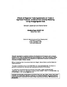
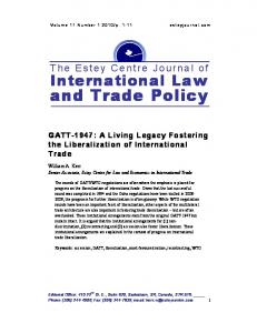
7. Results Impulse response function results The first task is to evaluate impulse responses from the model to see the effects that different policy shocks have on the Kitale and Nairobi prices. Key impulse responses from the model are shown in Figure 1. The impulse responses refer to the effect of a one time random shock in the impulse variable with all future random shocks to all variables set to zero. A positive shock to the NCPB purchase price premium increases both the Kitale and Nairobi prices and these increases are very persistent. This is as expected because an increase in the NCPB purchase price relative to the market price should lower supply delivered to non-NCPB markets and put upward pressure on Kitale prices. The increase in Kitale prices will then feed through into higher Nairobi market prices to the extent that these markets are integrated.

7

There is some weak evidence of low-order conditional heteroscedasticity in the Kitale price equation. However it is unlikely there would be conditional heteroscedasticity in the Kitale price but not the Nairobi or Mbale prices. We therefore assumed a time-invariant covariance matrix for the model’s residual vector.

23

40

Purchase Premium on Kitale Price

Purchase Premium on Nairobi Price

Sales Premium on Kitale Price

Sales Premium on Nairobi Price

Net Purchases on Kitale Price

Net Purchases on Nairobi Price

20

0

-20

40

20

0

-20 0

5

10

15

20

0

5

10

15

20

0

5

10

15

20

Step

Figure 1.

Impulse Response Functions

A positive shock to the NCPB sales price premium causes a persistent increase in the Nairobi price but a much more muted effect on Kitale prices (although Kitale prices do eventually rise). This is also consistent with economic logic because the higher NCPB sale prices are relative to the market price the less demand there will be for NCPB owned maize and the more demand there will be for maize coming to Nairobi through market channels. This upward pressure on Nairobi prices will eventually feed back into higher Kitale prices (though notice that this effect takes much longer than when the initial impact is in the production region, which suggests information flows more freely from Kitale to Nairobi than vice versa). Positive shocks to net NCPB purchases have negative effects on both Kitale and Nairobi prices, although the impact dies our quickly after six months or so. This might seem counterintuitive because we would expect that when the NCPB adds to stocks then 24

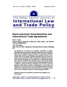
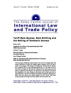
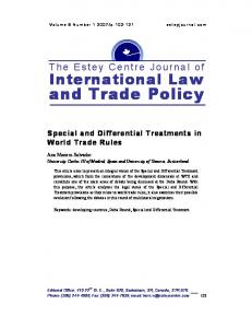
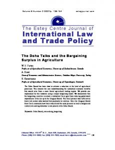
prices should rise. We have to remember, however, that this is the dynamic effect of a positive but unexpected random shock to net NCPB purchases, assuming no other shocks to the market but allowing all other equilibrium adjustments to the shock to take plus. Hence, it makes sense that if there is a positive unexpected shock to NCPB purchases there is an expectation that (other things remaining equal) those additional net purchases have to be released onto the market in the future and so prices begin to fall in anticipation of coming NCPB stock run-downs. The main goal of this study is to simulate what historical maize price paths would have been in Kenya in the absence of NCPB activities and import tariffs. We begin by focusing on NCPB activities assuming the tariff remained in place. Then we examine the effect of the tariff assuming NCPB maintained its historical role. And finally we look at removing both the NCPB effect and the tariff effect together. The Effects of NCPB Activities Prices in the absence of NCPB activities were simulated by: (a) constructing a set of counterfactual policy shocks that generate zero values for all three of the NCPB policy variables over the entire sample period; (b) assuming that the shocks to the market variables remain at their actual values over the sample period; and (c) constructing dynamic forecasts of the Kitale and Nairobi maize price paths under the counterfactual policy shocks and actual market shocks. The resulting simulated price paths are tabulated in Table 5 and graphed against the actual path of Kitale and Nairobi prices in Figures 2 and 3. The historical effect of the NCPB over the entire sample period was to raise both Kitale and Nairobi prices (by an average of a little over 5%) and also to stabilize prices by substantially reducing their coefficient of variation (see Table 5). However, these summary statistics mask the very large NCPB impacts that were estimated to have occurred in particular periods (see Figures 2 and 3). The NCPB’s activities raised prices in some periods (when the NCPB prices reflected substantial premiums to the market) and lowered them in others (when their prices reflected substantial premiums to the market).

25

For example, in the initial phases of the cereal market reform program, from early 1989 to 1992, our results indicate that the NCPB’s activities propped up maize market prices by roughly 30 percent in Kitale and roughly 20 percent in Nairobi (Table 5). This was during a period when private wholesale marketing was developing after having been suppressed for decades. In 1992/93 and again in 1993/94, drought conditions in Kenya sent Nairobi market prices over Ksh 800 per bag ($US 250 per tonne) and NCPB selling prices represented steep discounts to the market during this period. Not surprising, our simulation results indicate that the NCPB’s activities between June 1992 and June 1995 exerted downward pressure on market prices (between 15 to 20 percent lower). NCPB purchase prices were also substantially below wholesale prices in Kitale and other surplus areas during this period. Part of the price reduction effect around 1993 and 1994 may also have been due to the major increase in unrecorded private maize importation during this period, which unfortunately could not be incorporated into the model for lack of available data. After the maize market was ostensibly fully liberalized in 1995, the simulation results support the conventional wisdom in Kenya that the NCPB’s activities have served to raise maize market prices. Between July 1995 and June 2004, the model results indicate that NCPB raised wholesale market prices in both Kitale and Nairobi by roughly 16 percent. Interestingly, this impact on the market does not appear to have been achieved mainly through the shifting of marketed maize from market to NCPB marketing channels because NCPB’s actual purchases have been relatively modest during the post 1995 period. The two parallel marketing channels do not appear to be highly substitutable. Rather, it seems as though the NCPB’s price announcements (which have exceeded the market price by 10-15 percent in most years since 1995) influence perceptions and behavior of market participants in such a way as to raise open market prices mainly by the possibility of using the NPBP as a selling and buying option. Throughout the sample period, the NCPB appears to have dampened price variability in the wholesale markets. During drought years, it has normally sold heavily at deep price discounts to the market, and during bumper harvests its prices have tended to be higher than market prices. However, we cannot infer that the NCPB has reduced price uncertainty or price risk for producers. Some price instability (e.g., a seasonal

26

2000

1500 P R I C 1000 E 500

0 1989m

1993m

1997m Historical

2001m

2005m

No NCPB

Figure 2. Historical and Simulated (No NCPB) Kitale Prices

27

2000

1500 P R I 1000 C E 500

0 1989m3

1993m5 Historical

1997m7

2001m9

2005m11

No NCPB

Figure 3. Historical and Simulated (No NCPB) Nairobi Prices

28

Table 5. Summary of NCPB Effects on Kitale and Nairobi Wholesale Maize Prices, Nominal Ksh per 90kg bag Period

Kitale wholesale maize price (Ksh per 90kg bag)

Nairobi wholesale maize price (Ksh per 90kg bag)

Historical

No NCPB

% difference

Historical

No NCPB

% difference

April 1990 – May 1992 Mean Standard deviation Coefficient of variation

335.24 101.61 30.3%

256.19 99.35 38.8%

30.8% 2.3% -21.8%

422.58 53.77 12.7%

349.81 81.13 23.2%

20.8% -33.7% -45.1%

June 1992 – June 1995 Mean Standard deviation Coefficient of variation

723.20 216.83 30.0%

913.05 345.15 37.8%

-20.8% -37.2% -20.7%

898.76 164.34 18.3%

1080.71 347.07 32.1%

-16.8% -52.6% -43.1%

July 1995 – June 2004 Mean Standard deviation Coefficient of variation

996.71 308.09 30.9%

855.33 361.61 42.3%

16.4% -14.8% -26.8%

1212.56 277.27 22.9%

1048.81 384.06 36.7%

15.7% -27.8% -37.6%

Overall sample period (April 1990 – June 2004) Mean Standard deviation Coefficient of variation

848.56 355.34 41.9%

807.22 400.42 49.6%

5.1% -11.3% -15.5%

1033.64 365.58 35.4%

980.00 430.56 43.9%

5.5% -15.1% -19.4%

Note: “Historical” refers to actual prices; “no NCPB” prices are simulated from model results. Source: Ministry of Agriculture Market Information Bureau for actual prices; model simulation results for “no NCPB” prices.

29

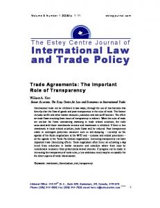
component to provide incentives for storage throughout the year) is to be expected and actually necessary to induce actors to undertake important marketing functions. Hence, the net impact of the NCPB on the predictability of the market cannot be inferred from these results. The Effects of the Tariff The tariff is included in the model via an adjustment to Ugandan prices to ensure these prices reflect the formal tariff cost of importing maize into Kenya. Within this framework, a simple way of simulating the effects of eliminating the tariff would be to re-adjust the Mbale, Uganda prices, period by period, to extract out the effect of the tariff, and then construct dynamic forecasts of the Kitale, Nairobi, and Ugandan maize price paths under the counterfactual assumption of no tariff. For now we set all other market and policy shocks to their historical levels (i.e. we assume the NCPB was implementing its historical policy rules. The resulting simulated price paths are tabulated in Table 6 and graphed against the actual path of Kitale and Nairobi prices in Figures 4 and 5. The tariff was estimated to have raised average Kitale prices by 2.5% over the sample period and average Nairobi prices by 1.8% . Not surprisingly, the effect of the tariff was almost zero in periods where the tariff was zero but higher when the tariff is higher. Also not surprisingly, the tariff has very little effect on Kenyan maize price variability over an extended period of time (see Table 6). These tariff effects may seem fairly minor given that the tariff was at times as high as 33%. However, as indicated earlier, there are several reasons why we would not expect Kenyan prices to differ from eastern Ugandan prices by an amount equal to the official tariff rate. First, it is widely believed that a substantial share of total imports from Uganda and Tanzania is smuggled into Kenya in an attempt to evade official border crossings (Awuor, 2003; RATES, 2004). Although such activities are likely to involve additional marketing costs, they presumably are lower than the costs that would otherwise be incurred by crossing through official border crossings, otherwise traders would not resort to such activities. Second, two focus group interviews of traders in 2004 reveals that there appear to be informal agreements between traders and border officials whereby the trader pays less (sometimes considerably less) than the official tariff rate on

30

2000 0

P KT/PK TSIM1 500 1000 1500 19 89 m3

1993m5

1997m7 MOVAR PKT

20 01 m9

2005m11

PKT SIM1

Figure 4. Historical and Simulated (No Tariff) Kitale Prices

31

2000 0

P N R/ PN R S IM 1 500 1000 1500 19 89 m3

1993m5

1997m7 MOVAR PNR

20 01 m9

2005m11

PNR SIM1

Figure 5. Historical and Simulated (No Tariff) Nairobi Prices)

32

Table 6. Summary of Maize Import Tariff Effects on Kitale and Nairobi Wholesale Maize Prices, Nominal Ksh per 90kg bag Period



Historical

No NCPB

% difference

Historical

No NCPB

% difference


335.35 101.61 30.3%

308.95 104.84 33.9%

8.5% -3.1% -10.7%

422.58 53.77 12.7%

395.73 58.39 14.8%

6.5% -7.9% -13.6%


723.20 216.83 30.0%

721.36 222.30 30.82%

0.3% -2.5% -2.7%

898.76 164.34 18.3%

898.31 170.59 19.0%

0.0% -3.7% -3.7%


996.71 308.09 30.9%

968.41 303.08 31.3%

2.9% 1.7% -1.2%

1212.56 277.27 22.9%

1188.26 274.64 23.1%

2.0% 1.0% -1.1%


848.56 355.34 41.9%

827.72 351.47 42.5%

2.5% 1.1% -1.4%

1033.64 365.58 35.4%

1015.43 363.63 35.8%

1.8% 0.5% -1.2%


maize importation.8 Third, in at least two marketing years trade flows were reversed due to weather disturbances in Uganda, causing the Kenyan import tariff to be irrelevant. For all of these reasons, we would expect that the net impact of the tariff on wholesale maize prices in Kenya would be less than the formal tariff rate (which fluctuated between zero and 35 percent over the sample period, but was 25-35% in most months. During some years, e.g., 1990/91 and 1998/99 marketing year, the import tariff raised Kenyan maize prices by 7-10 percent, but in most years, the estimated impact was negligible.

8

The advantage of the second process, from the standpoint of the trader, is that he/she obtains a form indicating formal customs clearance of the maize, which reduces the likelihood of having to pay bribes later at subsequent checkpoints in the way to Nairobi or other demand centers.

33

Joint Effects of the NCPB and the Tariff The counterfactual scenario of netting out the combined NCPB and tariff effects on prices results in graphs that are very similar to Figures 2 and 3 and so we do not report graphs for the combined case. However, the summary effects are provided in Table 7. We see that average prices were raised even higher by the joint effects of the policies, and prices were stabilized as well. As in the NCPB-only case there is a distribution of effects over time with prices being raised above what they would have otherwise been in most periods except the 1993-95 period when the NCPB was selling maize at a major discount to the market. Table 7. Summary of Cumulative NCPB and Maize Import Tariff Effects on Kitale and Nairobi Wholesale Maize Prices, Nominal Ksh per 90kg bag Period



Historical

No NCPB

% difference

Historical

No NCPB

% difference


335.24 101.61 30.3%

227.81 101.04 44.5%

47.6% 0.6% -31.8%

422.58 53.77 12.7%

320.40 86.73 27.1%

31.6% -38.0% -52.9%


723.20 216.83 30.0%

911.41 349.32 38.33%

-20.7% -37.9% -21.8%

898.76 164.34 18.3%

1081.20 352.23 32.58%

-16.9% -53.3% -43.9%


996.71 308.09 30.9%

831.79 347.84 41.8%

19.7% -11.4% -26.0%

1212.56 277.27 22.9%

1027.33 371.91 36.2%

18.0% -25.4% -36.8%


848.56 355.34 41.9%

787.83 397.69 50.5%

7.7% -10.6% -17.0%

1033.64 365.58 35.4%

963.19 429.33 44.6%

7.3% -14.8% -20.7%


34

8. Conclusions The objectives of this paper are to determine the effects of NCPB maize trading activity and the maize import tariff on wholesale maize market price levels and volatility. The analysis uses monthly maize price and trade data covering the period January 1990 to September 2004. Results are based on a vector autoregression (VAR) approach that allows estimation of a counterfactual set of maize prices that would have occurred over the 1990-2004 period had the NCPB not existed and trade restrictions been removed. In cases where a subset of variables in a structural econometric model are unobservable a legitimate “partially reduced form” model can be specified based on the relevant variables that are observed. This model is not as informative as the original structural model and the equations do not have the original structural interpretation as supply, demand, and policy equations. Nevertheless, the partially reduced form summarizes historical correlations and interactions among the observable variables and can still provide some useful insights. In particular, imposing a Choleski factorization or other means to identify the contemporaneous relationships among the endogenous variables allows identification of a set of policy shocks without putting any restrictions on the dynamic interrelationships between the variables in the system. These policy shocks can then be used to construct a counterfactual price path that would have existed under an alternative hypothetical path for the policy shocks, again, leaving the dynamics of the system essentially unrestricted. There are two main disadvantages to this approach. First, while it can estimate the net effect of a policy shock on the path of Kenyan maize prices it cannot provide definitive information about the mechanism that brings about that net effect (e.g. it cannot tell us whether the effect is primarily a supply effect or primarily a demand effect). Second, this modeling approach is very data intensive and the number of parameters to estimate can grow quickly to an unmanageable level, particularly if one were attempt to apply the approach to a regional model with four or more regions. Despite these disadvantages, the approach has been used successfully to evaluate policy effects in both macroeconomic models and microeconomic commodity market

35

models (see, for example, Bernanke, 1986 and Myers, Piggott and Tomek, 1990). And in cases like the Kenyan maize market where many of the variables required to estimate a full structural economic model are not observable, an approach based along these lines would seem to be the only viable econometric method available. Results of the VAR modeling and counterfactual simulations indicate that the NCPB’s activities have indeed had a marked impact on both maize price levels and volatility. The NCPB’s price setting and market operations have, on average, raised wholesale market prices in Kitale (a major surplus production area) and Nairobi (the main urban center) by 5.1 and 5.5 percent, respectively, over the entire sample period. However, the NCPB’s impact on the market varied considerably over different periods, being negative during the 1992/93 drought year and the 1993/94 year, when the NCPB was both buying and selling maize at a discount to market prices. Since the 1995/96 season, NCPB operations are estimated to have raised Kitale and Nairobi maize prices by 16.4 and 15.7 percent, respectively, implying a transfer of income from maize purchasing rural and urban households to relatively large farmers who account for roughly half of the country’s domestically marketed maize. The NCPB’s activities have also reduced the standard deviation and coefficient of variation of prices as well, consistent with its stated mandate of price stabilization. The maize import tariff, on the other hand, appears to have exerted only modest effects on open market maize price levels. Despite being set at 20 to 30 percent over the sample period, the tariff appears to have raised market maize price levels by only 2 to 3 percent.

The relatively weak impact of the tariff is likely to be due to apparently

widespread maize smuggling across borders, informal arrangements at border crossings that reduce effective tariff rates, and trade reversals in several years. These factors would presumably weaken or decouple the relationship between Uganda and Kenyan prices that otherwise might be expected if Ugandan maize consistently supplied Kenya, and if the official tariff were strictly enforced. In addition, the unavailability of key data, such as informal trade flows from Tanzania and Uganda constitute omitted information that may affect model results. The results imply very important income distributional effects arising from Kenya maize marketing and trade policy. Because 70 percent of Kenya’s maize surplus is

36

believed to be produced by roughly 1 percent of the farm population (mainly large farmers in the North Rift Valley), and because 65 percent of the rural small-scale farm families are typically net buyers of maize, policies that raise maize price levels are likely to have highly concentrated benefits and anti-poor distributional effects. However, rural households’ position in the maize market alone is not sufficient to determine the general equilibrium effects of maize pricing policy on welfare and income distribution. This is an important topic for further research.

37

References Ackello-Ogutu, C. and P. Echessah. 1997. Unrecorded Cross-Border Trade Between Kenya and Uganda. Technical Paper 59, SD Publication Series, Office of Sustainable Development, Africa Bureau, USAID, Washington, D.C. Awour T. A. 2003. Competitiveness on Maize Production from Western Kenya and Eastern Uganda in Kisumu Town of Kenya. MSc Thesis, Michigan State University through Tegemeo Institute, Nairobi, Kenya. Bernanke, B.S. (1986) “Alternative Explanations of the Money-Income Correlation.” Carnegie Rochester Conference Series on Public Policy 25: 49-100. Bernanke, B.S and I. Mihov (1998) “Measuring Monetary Policy.” The Quarterly Journal of Economics 113(3): 869-902. Fackler, P.L. (1988) “Vector Autoregressive Techniques for Structural Analysis.” Revista de Analisis Economico 3(2): 119-134. Greer, J. and E. Thorbecke. 1986. Food Poverty and Consumption Patterns in Kenya. Geneva: International Labour Office. Hamilton, J.D. (1994) Time Series Analysis. Princeton: Princeton University Press. Jayne, T.S., T. Yamano, J. Nyoro, and T. Awuor. 2001. Do Farmers Really Benefit From High Food Prices? Balancing Rural Interests in Kenya’s Maize Pricing and Marketing Policy. Working Paper 2b, Tegemeo Institute, Nairobi, Kenya. On-line at: http://www.aec.msu.edu/agecon/fs2/kenya/index.htm Karanja, D. and M. Renkow. 2003. The Welfare Effects of Maize Technologies in Marginal and Favored Regions of Kenya. Unpublished draft paper under review. Michigan State University, East Lansing, MI. Myers, R.J., R.R. Piggott, and W.G. Tomek (1990) “Estimating Sources of Fluctuations in the Australian Wool Market: An Application of VAR Methods.” Australian Journal of Agricultural Economics 34(3): 242-262. Nyoro J.K and Mary W Kiiru and T.S Jayne. 1999: Evolution of Kenya’s Maize Marketing systems in the Post Liberalization Era. A paper prepared in a joint collaboration with Tegemeo Agricultural Monitoring and Policy Analysis (TAMPA) Project, Egerton University/ Michigan State University with the support by the United States Agency for International Development/Kenya. On-line at: http://www.aec.msu.edu/agecon/fs2/kenya/index.htm

38

Nyoro, J.K., Lilian Kirimi, and T.S. Jayne. 2004. Competitiveness of Kenya and Ugandan Maize Production: Challenges for the Future. Working Paper 10, Egerton University, Tegemeo Institute, Nairobi. Online at: http://www.aec.msu.edu/agecon/fs2/kenya/index.htm RATES. 2003. Maize Market Assessment and Baseline Study for Kenya, April 2003. Center for Regional Agricultural Trade Expansion Support, Nairobi. Republic of Kenya. 2001. Statistical Abstract, Government Printer, Nairobi. Sims, C.A. (1980) “Macroeconomics and Reality.” Econometrica 48(1): 1-48.

39