J. Adv. Model. Earth Syst., Vol. 2, Art. #3, 21 pp.
Effects of Resolution on the Simulation of Boundary-layer Clouds and the Partition of Kinetic Energy to Subgrid Scales Anning Cheng1, Kuan-Man Xu2 and Bjorn Stevens3,4 1
Science Systems and Applications, Inc., Hampton, Virginia Climate Science Branch, NASA Langley Research Center, Hampton, Virginia 3 Max Planck Institute for Meteorology, Hamburg, Germany 4 Department of Atmospheric and Oceanic Sciences, University of California, Los Angeles, Los Angeles, California 2
Manuscript submitted 27 August 2009; in final form 25 January 2010
Seven boundary-layer cloud cases are simulated with UCLA-LES (The University of California, Los Angeles – large eddy simulation) model with different horizontal and vertical gridspacing to investigate how the results depend on gridspacing. Some variables are more sensitive to horizontal gridspacing, while others are more sensitive to vertical gridspacing, and still others are sensitive to both horizontal and vertical gridspacings with similar or opposite trends. For cloud-related variables having the opposite dependence on horizontal and vertical gridspacings, changing the gridspacing proportionally in both directions gives the appearance of convergence. In this study, we mainly discuss the impact of subgrid-scale (SGS) kinetic energy (KE) on the simulations with coarsening of horizontal and vertical gridspacings. A running-mean operator is used to separate the KE of the high-resolution benchmark simulations into that of resolved scales of coarse-resolution simulations and that of SGSs. The diagnosed SGS KE is compared with that parameterized by the Smagorinsky-Lilly SGS scheme at various gridspacings. It is found that the parameterized SGS KE for the coarse-resolution simulations is usually underestimated but the resolved KE is unrealistically large, compared to benchmark simulations. However, the sum of resolved and SGS KEs is about the same for simulations with various gridspacings. The partitioning of SGS and resolved heat and moisture transports is consistent with that of SGS and resolved KE, which means that the parameterized transports are underestimated but resolved-scale transports are overestimated. On the whole, energy shifts to large-scales as the horizontal gridspacing becomes coarse, hence the size of clouds and the resolved circulation increase, the clouds become more stratiform-like with an increase in cloud fraction, cloud liquid-water path and surface precipitation; when coarse vertical gridspacing is used, cloud sizes do not change, but clouds are produced less frequently. Cloud fraction and liquid water path decrease. DOI:10.3894/JAMES.2010.2.3 1. Introduction Boundary-layer clouds are parameterized in general circulation models (GCMs) because they are too small to resolve given even the most highly resolved representation of the global atmosphere. Even at the gridspacings used in the cloud resolving model (CRM) component of the Multi-scale Modeling Framework (MMF, Randall et al. 2003) or in a state of the art global cloud resolving model (GCRM, Tomita and Satoh 2004), circulations associated with boundary layer clouds are wholly unresolved. In an MMF, a CRM is embedded in each grid cell of the parent GCM to This work is licensed under a Creative Commons Attribution 3.0 License.
represent cloud physical processes. While the finest gridspacings used in traditional GCMs tend to be many tens of kilometers in the horizontal, both the MMF and GCRMs employ gridspacings of a few kilometers. Finer meshes can be employed as computational capacity permits. Since the gridspacing helps determine the extent to which the small scale processes are resolved, it is important to understand the effects of gridspacing on the simulation of boundarylayer clouds so as to better guide the use of the MMF (or GCRM) to represent the boundary-layer cloud processes. To whom correspondence should be addressed. Dr. Anning Cheng, 1 Enterprise Parkway, Suite 200, Hampton, VA 23666, USA
[email protected]
JOURNAL OF ADVANCES IN MODELING EARTH SYSTEMS
2
Cheng et al.
Studies on the sensitivities of simulation of boundarylayer clouds to gridspacing have usually focused on a single boundary-layer cloud case. Simulations have been performed with gridspacings less than 100 m in the horizontal and less than 40 m in the vertical direction in order to well resolve boundary layer circulations on scales of many hundreds of meters. The simulated results usually did not converge with a decrease in gridspacing in either direction. Stevens and Bretherton (1999) and Stevens et al. (2000) found that the thickness of the inversion, the depth of entrainment zone, and the shape of vertical velocity spectra were sensitive to the size of the horizontal and vertical mesh across the range of sizes they explored. Using a gridspacing range from 80 m to 10 m in the horizontal and from 40 m to 5 m in the vertical in simulations of a cumulus cloud regime capped by stratiform clouds, Stevens et al. (2002) pointed out that the mean cloud fraction, optical depth, and vertical fluxes of heat, moisture, and momentum are sensitive to numerical representation (grid spacing and choice of numerical methods) even for cases with relatively high resolution. The importance of the subgrid scale (SGS) parameterization on the convergence of the results from simulations with different gridspacings in the typical LES range has also been noticed. Here we distinguish between LES and CRMs. LES is designed to resolve the large-eddies of boundary layer turbulence, and hence has gridspacings smaller than the depth of the boundary layer (i.e., on the order of tens of meters); CRMs have grids chosen to help resolve the convective overturning of the troposphere, and hence feature gridspacings ranging from hundreds of meters to a few kilometers. Stevens et al. (1999) found that results from a SGS parameterization based on turbulence kinetic energy (TKE) are less sensitive to gridspacing than those from a Smagorinsky-Lilly SGS parameterization (Smagorinsky 1963) for a smoke cloud case. Stevens et al. (2002) also reported that the entrainment rate is dependent on SGS mixing for a stratocumulus case. More sophisticated turbulence closure schemes appear to reduce the dependence of CRM results on gridspacing. For instance, Cheng and Xu (2008) found that the vertical profiles of the total sensible and latent heat transports and cloud fraction are less sensitive to resolution for a CRM with a higher-order turbulence closure than one with a TKE SGS model because the higher-order turbulence SGS model more realistically absorbs the additional subgrid energy that is implied as the base grid is coarsened. An important factor that determines the quality of a SGS parameterization (at least for eddy-diffusivity based schemes) is the SGS TKE (Stevens et al. 1999). As the resolution of a simulation is degraded, the SGS TKE is expected to carry an increasing fraction of the transport, as well as mediate other processes, such as the coupling between cloud and radiative processes. Although some studies have explored the role of entrainment on the growth JAMES
Vol. 2
2009
and dissipation of boundary-layer clouds (e.g., Stevens and Bretherton 1999; Stevens et al. 2002), with a few notable exceptions (i.e., Mason and Brown, 1999) less attention has been paid on whether the SGS kinetic energy (KE) increases as one would expect as resolution is degraded from the typical LES to CRM range. The partition of KE into SGS and resolved-scale across a range of gridspacings and the impact on the vertical transports has not been systematically explored. Note that both SGS and resolved KEs to be extensively discussed in this study exclude the KE produced by the large-scale mean wind. The SGS KE belongs to TKE, while the resolved KE may include components from mesoscale circulations typically not associated with turbulence. Further discussion on the relationships among various scales will be given in section 3. The primary objectives of this study are 1) to systematically study how important aspects of simulated cloud-topped boundary layers change across a range of gridspacings used in LES, CRM, and the MMF for the major GEWEX (Global Energy and Water-cycle Experiment) Cloud System Study (GCSS) cases, and 2) to investigate the consistency with which energy is partitioned between the resolved and SGS at these varying resolutions and the impact of this energy partitioning on the vertical transports when boundary-layer clouds are present. We do so by exploring two classes of cloud-topped boundary layers: layers of shallow cumulus, and stratocumulus. In total we study seven different cases, but focus our analysis on two prototype cases, one of cumulus and the other of stratocumulus. The remaining simulations are then explored to help generalize our main findings. The rest of the paper is organized as follows. Section 2 provides the model description and experiment design. Results are presented in Section 3, and conclusions in Section 4. 2. Model description and experiment design The CRM used for this study was developed most recently at the University of California, Los Angeles (UCLA, Stevens et al. 1999). It represents the flow in the anelastic approximation with periodic boundary conditions in each horizontal direction. Free slip boundary conditions are set at the surface and model top. A fourth-order centered difference scheme is used to represent momentum advection on the three components of the velocity vector, and a monotone upwinding method is used for the advection of scalars. The scalars include the liquid-water potential temperature, the total water mixing ratio, the mass mixing ratio of rain water, and the number concentration of rainwater drops. Condensation is accounted for by a saturation adjustment (‘‘all or nothing’’) scheme in which cloud water is diagnosed as the difference between total water and saturation mixing ratio. Details of the cloud microphysical processes were discussed in Stevens and Seifert (2008) and Savic-Jovcic and Stevens (2008). The Smagorinsky-Lilly subgrid model is used to represent subgrid fluxes of both scalars and adv-model-earth-syst.org
Simulation of boundary-layer clouds
3
Table 1. Summary of GCSS cases performed in this study. Cases
Full name
BOMEX
Barbados Oceanographic and Meteorological Experiment Atmospheric Radiation Measurement Rain In Cumulus over the Ocean Atlantic Trade Wind Experiment Atlantic Stratocumulus Transition Experiment The Second Dynamics and Chemistry of Marine Stratocumulus field study – first research flight The Second Dynamics and Chemistry of Marine Stratocumulus field study – second research flight
ARM RICO ATEX ASTEX DYCOM-RF01 DYCOM-RF02
Cloud type
References
Marine shallow cumulus
Siebesma et al. (2003)
Continental shallow cumulus Drizzling shallow cumulus Cumulus capped by stratus Stratocumulus over Atlantic ocean
Brown et al. (2002) Rauber et al. 2007 Stevens et al. (2001) Roode and Duynkerke (1997)
Stratocumulus over east Pacific Ocean
Stevens et al. (2005)
Drizzling stratocumulus over east Pacific Ocean
Ackerman et al. (2009)
momentum. The radiative heating rates for the cases studied here are either prescribed or calculated using a simple flux parameterization that is dependent only on liquid water path. No short-wave radiation is included. A total of seven GCSS cases (Table 1) have been selected for this work. These cases span a large range of boundarylayer cloud regimes and produce cloud layers with a wide range of cloud fractions, liquid and rain water. They consist of two non-drizzling (ARM and BOMEX) and a drizzling (RICO) fair-weather cumulus cloud cases, two non-drizzling (ASTEX and DYCOM-RF01) and a drizzling (DYCOMRF02) stratocumulus-topped marine boundary cloud cases, and a mixed case (ATEX) of cumulus rising underneath a broken stratocumulus deck. The ARM case is a continental shallow cumulus observed from the Southern Great Plains (SGP) measurement site maintained by the Department of Energy Atmospheric Radiation Measurement Program (ARM). The rest of the cases are marine boundary-layer clouds. BOMEX, RICO, ASTEX, and ATEX are based upon observations taken from Atlantic Ocean and DYCOM-RF01 and –RF02 are from measurements in the stratocumulus cloud fields of the Northeast Pacific (Stevens et al. 2005). All simulations to be described below use the same initial conditions and forcings as the standard GCSS specification. A complete description of the intercomparison cases can be found in the original references, which we list in Table 1. We only briefly outline some salient features here. Largescale horizontal temperature and moisture advective tendencies are prescribed for all cases, as is a vertical motion field for calculating vertical advective fluxes given the mean fields. Time-varying surface latent and sensible heat fluxes derived from observations are used to force the model for the ARM case, with a maximum value of 500 W m22 for the latent heat flux and 140 W m22 for the sensible heat flux at local noon, in order to simulate diurnal variations of continental boundary-layer clouds. Constant surface latent and sensible heat fluxes were prescribed for BOMEX and ASTEX cases while constant sea surface temperatures (SSTs) were prescribed for the remaining marine cases. In three shallow cumulus cases (ARM, BOMEX, and RICO) the radiative cooling rate was prescribed, but similar to what
was done in the original inter-comparison studies a simple radiative flux parameterization based on liquid water path (Stevens et al. 1999) was used in the rest of the cases. To investigate how the results change as the gridspacing is coarsened, the horizontal and vertical gridspacings are varied from half of the value that was used in the original intercomparisons to the much coarser gridspacings typical of MMF and GCRM studies (Fig. 1). Uniform horizontal gridspacings ranging from 50 m to 4 km are used for all the cases. For the pure cumulus cases uniform grids were also used in the vertical, with gridspacings ranging from 20 to 320 m. For the stratocumulus cases, including ATEX, stretched grids were used in the vertical. These were prescribed so that vertical resolution along the finest part of the
Fig. 1. A schematic description of the gridspacing sensitivity testing strategy for the seven GCSS cases. Here Dx0 and Dz0 refer to the standard GCSS gridsizes in the x/y and z directions, respectively. The green, red and blue points denote the fineLES, GCSS-LES (benchmark experiment), and control, respectively.
JOURNAL OF ADVANCES IN MODELING EARTH SYSTEMS
4
Cheng et al.
Table 2. Summary of gridspacings used in the experiments performed in this study. The finest gridspacings in the vertical direction near inversion are shown for the stratocumulus cases. Cases
Benchmark experiments
BOMEX ARM RICO ATEX ASTEX DYCOM-RF01 DYCOM-RF02
100 m 6 100 m 6 40 m 100 m 6 100 m 6 40 m 100 m 6 100 m 6 40 m 100 m 6 100 m 6 40 m 50 m 6 50 m 6 25 m 50 m 6 50 m 6 5 m 50 m 6 50 m 6 5 m
Fine-LES 50 50 50 50 25 25 25
m m m m m m m
6 6 6 6 6 6 6
50 50 50 50 25 25 25
m m m m m m m
6 6 6 6 6 6 6
grid (around the temperature inversion which demarcates cloud top) varied between 5 and 50 m. The coarsest part of the grid, typically near the model top, had resultant gridspacings ranging from 40 to 350 m. The horizontal domain size used for each simulation is determined so that the simulations no longer show an explicit, or at least strong, sensitivity to domain size. The domain size is usually a few kilometers by a few kilometers (e.g., 6.4 km by 6.4 km for BOMEX) when the horizontal gridsize is less than 100 m, but can increase to 64 km by 64 km when the horizontal gridsize is 4 km. The vertical extent of the domain is 4 km for the shallow cumulus cases, and is 1.5 km for the stratocumulus cases. 3. Results 3.1. A shallow cumulus – the RICO case The drizzling shallow cumulus case follows the case based on observations taken during the Rain In Cumulus over the Ocean field study (RICO, Rauber et al. 2007). The initial condition and large-scale advective forcing data for this case are derived by compositing over a three-week period from December 16, 2004 to January 8, 2005, in which shallow cumulus convection was active. The combined radiosondes and dropsondes show only a weak inversion with continuously high relative humidity (up to 70%) in the inversion layer and above (not shown). The large-scale heat and moisture tendencies due to horizontal advection, large-scale subsidence and radiative cooling, which are assumed to be time independent, are prescribed while surface fluxes are calculated with a fixed sea surface temperature of 299.8 K and simulated near-surface temperature and water vapor mixing ratio at surface pressure of 1015.40 hPa. The observed (spatially-averaged) rainfall rate during the threeweek period is about 0.3 mm day21. The horizontal gridsize used in the LES intercomparison study was 100 m in both xand y-directions, with a domain size of 12.8 km 6 12.8 km. A uniform vertical gridsize of 40 m was used, with a domain depth of 4 km. The total integration time was 24 h. A detailed description of the configuration of the RICO composite case can be found online at http://www.gewex. org/gcss.html. We also made a higher resolution LES experiment, denoted as fine LES, using half of the gridspacing of the intercomparison study, i.e., 50 m in the horizontal and JAMES
Vol. 2
2009
20 m 20 m 20 m 20 m 12.5 m 2.5 m 2.5 m
Control experiments
Sensitivity tests
Increase gridspacings in all directions, represented by the blue points in Fig. 1
Same as control runs except using the diagnosed SGS TKE
20 m in the vertical directions, respectively. Similar to what was found by Stevens and Seifert (2008), differences are relatively small between the standard and fine LES experiments compared with those between the standard experiments and the coarser gridspacing experiments (listed as control experiments in Table 2 and shown as blue points in Fig. 1). Hereafter, the standard experiments are also called ‘‘benchmark’’ experiments. 3.1.1. Mean thermodynamic profiles and energy spectra There are two main effects of decreasing horizontal resolution on the RICO case: one is to weaken the distinction between the cloud layer and the overlying free atmosphere; the other is to change the vertical structure of the cloud field itself, i.e., the primary peak of cloud fraction and liquid water shifts from the upper cloud layer to the cloud base. These features are evident in Fig. 2 which presents the mean profiles averaged over the last four hours. Six simulations are presented in which the horizontal gridspacing systematically increases from 100 m to 2 km with a fixed vertical gridspacing of 40 m. The weak inversion layer above cloud top gradually disappears, but cloud water, cloud fraction, and rainwater near cloud base increase when the gridspacing becomes coarse. Cheng and Xu (2008) attributed this gradual degradation to the stronger resolved circulations at the coarser resolution produced by the buildup of the convective available potential energy (CAPE) required to cause over-turning on the scales resolved by the model. The overturning circulations tend to be more buoyant, and hence more energetic, and thus more effectively erode the capping inversion layer. As a result, the cloud water above 3000 m is nonzero for the coarser resolution runs (Fig. 2c). More episodic, but somewhat more violent, convection is also consistent with lower liquid water potential temperatures and higher total water mixing ratios in the subcloud layer. These latter features are probably responsible for larger cloud water and cloud fraction near cloud base. The deep cloud layers in the coarse-resolution runs (including MMF run) are responsible for the large amount of rain water (Fig. 2e), which is initiated at higher altitudes than in the fine-resolution runs that have weaker resolved-scale circulations. Notice that the MMF experiment uses horizontal gridsize of 4 km, and vertical gridspacing larger than 100 m, and it produces fairly reasonable cloud water and adv-model-earth-syst.org
Simulation of boundary-layer clouds
5
Fig. 2. Sensitivities of mean profiles to the horizontal gridspacings: (a) liquid-water potential temperature, (b) total-water mixing ratio, (c) cloud water content, (d) cloud fraction, and (e) rain water averaged over the last four hours for the RICO case. The horizontal gridspacing used for MMF is 4 km, and the vertical grid levels below 4 km are located at 24.1 m, 142.9 m, 423.1 m, 905.1 m, 1605.2 m, 2545.1 m, and 3645.3 m, respectively.
cloud fraction near cloud base, the reason for this will soon become apparent. The sensitivities of the simulations to vertical gridspacing with the horizontal mesh fixed at 100 m can be seen in
Fig. 3. The inversion of liquid water potential temperature and hydro-lapse at cloud top are arguably less sensitive to changes in the vertical gridspacing. However, the cloud fraction and cloud water, especially near cloud base,
JOURNAL OF ADVANCES IN MODELING EARTH SYSTEMS
6
Cheng et al.
Fig. 3. Same as Fig. 2 except for different vertical gridspacings. Homogeneous vertical grid spacing is used for this case.
decrease for the coarser vertical grid runs, which is contrary to the effects of coarser horizontal gridspacings (Figs. 2c, d). If the horizontal gridspacing becomes coarse, cloud sizes increase; the clouds become more stratiform-like with an increase in cloud fraction and cloud water, which is conJAMES
Vol. 2
2009
sistent with the fact that Dx always tends to be larger than Dz. If the coarse vertical gridspacing is used, cloud sizes do not change, but clouds are produced less frequently (more discussions about this are given in Section 3c). The compensating effects of increasing the horizontal and vertical adv-model-earth-syst.org
Simulation of boundary-layer clouds
7
Fig. 4. Sensitivity of the power spectra of kinetic energy to horizontal gridspacing (a), and vertical gridspacing (b) at 1520 m for RICO.
gridspacings on the cloud fraction near cloud base may explain the reasonable cloud fraction from the MMF configuration with the increase of gridspacings in both directions at the same time. To link the sensitivity of the mean profiles to the resolved-scale circulations, the power spectra of the resolved KE are compared among the different simulations. As in the sensitivities shown in Figs. 2 and 3, the KE power spectra are also more sensitive to the horizontal gridspacing than to the vertical gridspacing (Fig. 4). A few other distinct features appearing in Fig. 4 can be pointed out. First, all the resolved energy very roughly follows the k25/3 slope, which is associated with a constant energy flux to high wavenumbers. The slope of the power-spectra at high wavenumbers differs among simulations with different horizontal resolutions. The steeper slope is associated with the simulations with a 100 m horizontal mesh, which means the energy is being removed quickly by the SGS processes. Second, the power of the spectra decreases with the increase of horizontal gridspacing for small scales (k . ,1024 m21), which measures the decrease in variance (or energy) of the resolved eddies for such scales; the opposite or nearly flat trend occurs when k , ,1024 m21. This means that the resolved KE shifts to large-scale when the horizontal gridspacing becomes coarse. In contrast, the power spectra for different vertical gridspacings are similar except for the simulation with 320 m vertical gridspacing, which is larger than the inversion thickness. Although the strong circulation of the resolved scales for the simulations with coarse horizontal resolution is directly responsible for the large differences among the mean thermodynamic profiles, cloud water, and cloud fraction, the power spectra of the kinetic energy from the resolved scale roughly follow the k25/3 slope. This suggests that the response
of the resolved scale may be physically reasonable but the coarser resolution is likely making the flow behave more viscously, and hence energy is removed from the flow too effectively. In the analysis presented below, we will focus on the role that kinetic energy plays in the vertical transport of heat and moisture and on the mean states when the horizontal and vertical gridspacings are systematically coarsened. 3.1.2. Partition of kinetic energy to subgrid scales and its effects 3.1.2.1. Diagnostic studies Before the results are discussed in the following section, it is helpful to clarify a basic concept in large-eddy modeling, namely, the subfilter scale, and its relationship with the grid scale and subgrid scale extensively discussed in this study. Formally one likes to derive the equations for LES by applying a filter to the equations. In principle the filter should remove all scales unrepresentable on the grid. This is what happens for spectral models where a precise truncation of scales can be made. In practice the LES equations are filtered imperfectly. That is, the combination of the numerics and the grid mesh define, implicitly, a filter. Such a filter tends not to have well defined characteristics, and it can be said that it is not spectrally precise. In particular the filter that is implicitly defined by model’s numerical algorithms not only cuts off scales smaller than the grid mesh, but it distorts scales near the size of the mesh. In this case the filter scale is loosely defined as somewhat larger than the mesh scale. A drawback of such definition of the filter scale is the inability to separate the effects on the total error due to numerical errors versus physical errors in the representation of subgrid-scale processes. The effective scale of LES—the resolved scale—is always much larger than the grid scale,
JOURNAL OF ADVANCES IN MODELING EARTH SYSTEMS
8
Cheng et al.
Fig. 5. SGS KE (a) and resolved KE (b) diagnosed using running mean operator from the benchmark experiment, parameterized by the Smagorinsky-Lilly SGS scheme (a), and simulated by the UCLA CRM (b) for gridspacings of 250 m, 500 m, 1 km, and 2 km that are averaged over the last four hours of RICO simulations. ‘‘D_’’ denotes diagnosed variables, and ‘‘P_’’ denotes the parameterized and simulated ones.
and typically somewhat larger than the filter scale. In our subsequent analysis our ability to partition between resolved and subgrid scale circulations is hampered by the fact that we do not know the precise size and characteristics of the filter implicitly defined by the LES. Hence we use a simpler approach, based on a running mean operator tied to the gridscale to be discussed below. Such operators have undesirable properties for the analysis we perform here (Reynolds averaging rules are not satisfied) but should suffice for the points we wish to make. More discussions about subgrid-scale and subfilter can be found in Mason and Brown (1999). A running-mean operator is used in both x and y directions to separate the kinetic energy of the benchmark simulation with the standard GCSS resolution into that of resolved scales corresponding to coarse-resolution simulations and that of SGSs. The running mean operator is n 1 X akzi . A new smoothed sequence, bk , defined by bk ~ 2n i~{n is generated from a sequence of numbers ak , where ak can be any variable, such as u, v, w, and TKE. The scale removed by such a filter is determined by n, the half range of the running mean. For example, if n55, scales less than 1000 m are filtered out given the gridsize used for the benchmark simulation is 100 m; if n52.5, scales less than roughly 500 m are removed by the filter. The filtered results provide a benchmark for comparison with those obtained by the coarse-resolution simulations (i.e., control experiments listed in Table 2) that use the Smagorinsky-Lilly SGS parameterization. The horizontal spacing range used for running-mean operator has rather consistent effects on the partition of JAMES
Vol. 2
2009
KE to SGS and resolved KE. The SGS KE increases and the resolved KE decreases as the horizontal spacing ranges become larger (Fig. 5). Slightly more than half of the total KE becomes SGS KE when the horizontal spacing range is 250 m, but most of the KE is partitioned to the SGSs when the horizontal spacing range is 2 km. The associated SGS liquid water potential temperature and moisture transports are primarily determined by the SGS KE (Fig. 6). SGS transports increase due to the increase in SGS KE as the horizontal spacing ranges become larger; the resolved transports, on the other hand, decrease correspondingly. The sum of SGS and resolved KE and the total transport are, by design, independent of the horizontal spacing range. The Smagorinsky-Lilly SGS parameterization is not supposed to reproduce the SGS KE and the SGS liquid water potential temperature and moisture vertical transports because it is not designed for use in simulations with horizontal gridspacings in which the main, isotropic, and energy containing eddies are not resolved. For an atmospheric boundary layer whose depth varies between 500 m and 2 km this corresponds to scales around 100 m. But it is nonetheless informative to examine the parameterized KE and the liquid water potential temperature and moisture vertical transports (Figs. 5 and 6). The SGS KE from the parameterization differ little among the control simulations with the horizontal gridspacings in the range from 250 m and 1 km, and fails to produce the maximum in SGS KE above cloud base (located at 600 m). As a result, the compensating resolved KE is unrealistically larger compared to the benchmark, especially in the cloud layer between 600 m and 2500 m. adv-model-earth-syst.org
Simulation of boundary-layer clouds
9
Fig. 6. Same as Fig. 5 except for vertical transports of liquid-water potential temperature (hl) and total-water mixing ratio (qt) of RICO simulations. The subgrid-scale transports (w 00 hl 00 , w 00 qt 00 ) are shown in (a) and (b) while the resolved transports (w 0 h0l , w 0 qt0 ) are shown in (c) and (d).
3.1.2.2. Sensitivity experiments In order to further investigate the impact of the energy partition on the vertical transports of liquid water potential temperature and moisture, we modify the eddy viscosity in the Smagorinsky-Lilly SGS parameterization by using the diagnosed SGS KE (Fig. 5a): pffiffiffi ð1Þ km ~0:18cs l e , where cs 5 0.23 is a constant, e~(u002 zv 002 zw 002 )=2 is the diagnosed SGS KE, and u00 , v 00 , and w 00 are the three components of the SGS velocity in x, y, and z directions, rffiffiffiffiffiffiffiffiffiffiffiffiffiffiffiffiffiffiffiffiffiffiffiffiffiffiffiffiffiffiffiffiffiffiffiffiffiffiffiffiffiffiffiffiffiffiffiffiffiffiffiffiffiffiffiffiffiffiffiffiffiffiffi .h i
respectively. l~
1
(DxDyDz){2=3 z(zk=cs ){2
is a
characteristic length-scale averaging between a grid-scale
and a length-scale proportional to the height above the surface, which allows km =(u 1 z) to approach k in the neutral surface layer (the log law), where k~0:35, and u 1 is the frictional velocity. The rest of the Smagorinsky-Lilly SGS scheme in the UCLA CRM remains unchanged. In the sensitivity experiments (Table 2), the diagnosed mean SGS KE for different horizontal spacing ranges was taken from the benchmark results and fed into the model. It is assumed that the SGS KE is stationary and horizontally homogeneous. Because the initial condition and forcing data used in the sensitivity experiments are chosen such that they are in balance and the turbulence is usually homogeneous in the horizontal directions, we suspect that these assumptions are not limiting. The initial conditions are the mean profiles at hour 20 from the benchmark simulation with specified random
JOURNAL OF ADVANCES IN MODELING EARTH SYSTEMS
10
Cheng et al.
Fig. 7. Same as Fig. 6 except from the sensitivity tests, in which the diagnosed SGS KE was used in the Smagorinsky-Lilly SGS parameterization to calculate the eddy viscosity in order to investigate the effects of the partition of KE to SGSs on the simulation of the vertical transports of liquid-water potential temperature and moisture. All variables are averaged over the four hours of the simulations.
perturbations. The horizontal gridspacings are chosen to be 250 m, 500 m, 1 km, and 2 km for the four sensitivity experiments. The horizontal domain size is 64 km, the vertical gridspacing is 40 m and the model top is set to 4 km for all four sensitivity experiments. The forcing data used are the same as the control experiments, which were described in Section 2. The integration time is 4 hours. The energy partitioning strongly affects the vertical liquid water potential temperature and moisture transports. Despite the simplicity of the parameterization of the eddy viscosity in (1), the SGS liquid water potential temperature and moisture transports at cloud base and cloud top increase, especially in the 1 km and 2 km gridspacing runs (Figs. 7a and b), compared to those of the control experiments (Fig. 6). Because SGS processes such as the condensaJAMES
Vol. 2
2009
tion and the associated transports are not considered in (1), the transports in the cloud layer are still underestimated. The effects of the ‘‘realistic’’ SGS KE on the resolved scale transports are also drastic (Figs. 7c and d). The resolved heat and moisture transports from the 250 m and 500 m gridspacing tests compare fairly well with the diagnosed profiles from the benchmark simulation. The resolved KE for the 1 km and 2 km gridspacing tests reduces to zero (the resolved transport for these two experiments collapse to one line in Figs. 7c and d). The increase in the SGS transports may be the reason for this result, which likely deprives the large-scales of the energy they require to overturn in these simulations. Because of the larger imposed SGS KE for calculating viscosity than in the control simulations, better convergence is evident in the mean profiles of liquid water potential adv-model-earth-syst.org
Simulation of boundary-layer clouds
11
Fig. 8. Same as Figs. 2a and 2b except for the sensitivity tests, in which the diagnosed SGS KE was used in the Smagorinsky-Lilly SGS parameterization to calculate the eddy viscosity.
temperature and total water for the four experiments (Fig. 8) as compared to those shown in Fig. 2. The mean profiles of cloud fraction, cloud amount, and rain water mixing ratio are, however, unrealistic (not shown) because SGS condensation and microphysics are neglected in the Smagorinsky-Lilly SGS parameterization, which are crucial for producing reasonable profiles of those variables. 3.2. A drizzling stratocumulus – the DYCOM-RF02 case The Second Dynamics and Chemistry of Marine Stratocumulus field study – second research flight (DYCOM-RF02) took place over the ocean to the westsouthwest of San Diego, California, July 2001 (Stevens et al. 2005). Drizzling stratocumulus clouds were observed in a well-mixed boundary layer with an average surface precipitation rate of 0.35 mm day21. The drizzle had noticeable effects on entrainment and liquid water path. Following the prescription of Ackerman et al. (2009), surface sensible and latent heat fluxes and large-scale subsidence are prescribed in the simulations performed in this study. A simple, interactive radiation scheme is included; the radiative flux is diagnosed from the predicted liquid water content. In this study, the gridspacings for this case range from 25 m to 4 km in the horizontal, and range from 2.5 m to 40 m near the height of inversion in the vertical, gradually becoming coarser away from the inversion. Although a CRM with a horizontal gridspacing of 1 km can produce 100% cloud fraction for an observed overcast stratocumulus cloud case (Cheng and Xu 2008), large eddies are still unresolved compared to high-resolution large-eddy simulations. The strong radiative cooling near the cloud top can lessen the effects of the resolution on the simulation of the stratocumulus clouds. The inversion was maintained for
the experiments with coarser horizontal and vertical gridspacings (Figs. 9a, b and Figs. 10a, b), in contrast to the RICO case. It seems that the resolved circulation is not strong enough to break up the strong inversion because of the strong cloud top radiative cooling. The cloud thickness and rainwater increase for the experiments with coarser horizontal gridspacing (Figs. 9c-e) due to slightly stronger resolved circulations and vertical transport similar to what was found for the RICO case. On the other hand, cloud water, thickness and rain water decrease for the experiments with coarser vertical gridspacings (Figs. 10c, e). The larger cloud top entrainment from the coarser vertical gridspacing experiments may contribute to the dissipation of the stratocumulus clouds (Bretherton et al. 1999). Similar to RICO, the diagnosed portion of SGS KE from the benchmark simulation increases consistently as the horizontal spacing range becomes larger (solid line in Fig. 11), but the partitioning is influenced by the strong radiative cooling near cloud top and the strong coupling between the cloud layer and the subcloud layer, which are two characteristics of stratocumulus clouds. Another difference from RICO is that the SGS KE near cloud top is much larger than that near cloud base and is not sensitive to the changes of the horizontal spacing ranges, especially near the inversion (above 900 m). Furthermore, the subcloud layer and cloud layer are not as distinguishable in the SGS and resolved KE profiles as those of RICO (Fig. 5), which indicates a more continuous coupling between the subcloud layer and the cloud layer for stratocumulus clouds. The diagnosed resolved and SGS liquid water potential temperature and moisture transports from the benchmark simulation are consistent with the diagnosed resolved and SGS KE, with small magnitudes of resolved transports and large magnitudes of SGS transports (solid lines in Fig. 12)
JOURNAL OF ADVANCES IN MODELING EARTH SYSTEMS
12
Cheng et al.
Fig. 9. Same as Fig. 2, except for DYCOM-RF02. The profiles were obtained from the averages over the last two hours of the simulations.
occurring in the larger horizontal spacing ranges. These transports near the inversion are also not sensitive to the horizontal spacing range, where the radiative cooling is the strongest. JAMES
Vol. 2
2009
Although its magnitude is smaller than that diagnosed from the benchmark simulation, the Smagorinsky-Lilly SGS scheme gives a relatively reasonable SGS KE in the control experiments for the DYCOM-RF02 case compared to RICO adv-model-earth-syst.org
Simulation of boundary-layer clouds
13
Fig. 10. Same as Fig. 3, except for DYCOM-RF02. The profiles were obtained from the averages over the last two hours of the simulations. The finest vertical gridspacings used at the inversion are shown in the legend.
(dashed lines in Fig. 11). For example, the maximum region of the SGS KE near cloud top is well captured, and the magnitude of SGS KE becomes larger as the horizontal gridspacing increases.
The Smagorinsky-Lilly SGS scheme, however, underestimates the SGS transports at the cloud top (dashed lines in Figs. 12a, b) and the cloud base. The underestimation of the SGS transport near cloud top may be due to the small eddy
JOURNAL OF ADVANCES IN MODELING EARTH SYSTEMS
14
Cheng et al.
Fig. 11. Same as Fig. 5, except for DYCOM-RF02. The profiles were obtained from the averages over the last two hours of the simulations.
viscosity, and the scheme is not expected to give reasonable transports near cloud base where the gradient of the mean profile is very small and thus a parameterization of nonlocal transports may become important. The resolved transports are overestimated at the cloud top and cloud base (Figs. 12c, d), and so is the resolved KE (Fig. 11b). To investigate the impact of energy partition on the vertical transports of liquid water potential temperature and moisture for the stratocumulus clouds, the diagnosed SGS KE from the benchmark simulation was used to calculate the eddy viscosity in the Smagorinsky-Lilly SGS parameterization as was done for the RICO case. The initial conditions are the mean profiles at hour 2 from the benchmark simulation with specified random perturbations. The horizontal gridspacings used are 100 m, 250 m, 500 m, and 1 km for the sensitivity tests. The horizontal domain size is 64 km, and the vertical gridsize is 5 m below and near the inversion stretched to 40 m at the model top at 1.5 km. The forcing data used are the same as the control experiments, as described in Section 2. The integration time is 2 hours. With the ‘‘realistic’’ SGS KE, the liquid water potential temperature and moisture transports near cloud top from the sensitivity tests increase and are more reasonable (dashed lines in Fig. 13) compared with those diagnosed from the benchmark simulation (solid line in Fig. 13). As a result, the resolved transports decrease compared with those from the control experiments (dashed lines in Figs. 12c, d). It is noted that the resolved transports from the 250 m and 500 m runs compare well with those diagnosed from the benchmark simulation for their respective horizontal gridspacings. A convergence of the mean profiles of liquid water potential temperature and total water for the four sensitivity tests can be also seen for the DYCOM-RF02 case (not shown). JAMES
Vol. 2
2009
3.3. Results from all cases The sensitivity of vertically integrated TKE, maximum domain vertical velocity, cloud fraction, liquid water path, surface precipitation flux, the inversion height, cloud base height, and surface latent heat flux to both horizontal and vertical gridspacings for the three GCSS shallow cumulus cases (BOMEX, RICO, and ARM) and for the four stratocumulus cases (ASTEX, ATEX, DYCOM-RF01 and -RF02) are shown in Figs. 14 and 15, respectively. The differences between the control and the benchmark experiments (Fig. 1) of each variable are summed and averaged over the shallow cumulus and the stratocumulus cases, respectively. The sensitivities of the results to gridspacings fall into four categories depending on the statistic: more sensitive to horizontal gridspacing, more sensitive to vertical gridspacing, and sensitive to both horizontal and vertical gridspacings with similar or opposite trends. For instance, the surface latent-heat flux is most sensitive to the vertical gridspacing when it is larger than 3Dz0 for stratocumulus cases (Fig. 15h), where Dz0 is the vertical gridspacing of the benchmark simulation, while the vertically integrated TKE appears to depend more on horizontal gridspacing for the shallow cumulus cases (Fig. 14a), which is consistent with the power spectra shown in Fig. 4. Domain-maximum vertical velocity (wmax) is sensitive to both the horizontal and vertical gridspacings for all cases, and has the same trend: wmax decreases for the coarser gridspacings. Cloud fraction and liquid water path have an opposite dependence on the vertical and horizontal gridspacings (Figs. 14c, d and 15c, d): they increase with coarser horizontal gridspacing, but decrease with coarser vertical gridspacing. Most cloud-related variables have the opposite dependence on horizontal and vertical gridspacings, such as cloud fraction, liquid water path, and adv-model-earth-syst.org
Simulation of boundary-layer clouds
15
Fig. 12. Same as Fig. 6, except for DYCOM-RF02. The profiles were obtained from the averages over the last two hours of the simulations.
the height of cloud base, implying that changing the gridspacing proportionally in both the horizontal and vertical will lead to compensating effects and minimal overall changes. This is also the case for surface latent heat flux if the vertical gridspacing is not too large for the stratocumulus cases. In order to further understand the dependence of results on gridspacing, the dependence of the mean diameter of the clouds, the ratio of the diameter to the height, and the number of clouds in a 256 km by 256 km box (Nr) on the grid spacings for the three shallow cumulus cloud cases are presented in Fig. 16. The size and Nr of the clouds for stratocumulus cases (not shown) are qualitatively similar to shallow cumulus clouds except with larger diameters of the clouds and lower Nr. Note that the cloud size is calculated in each cloudy model level and averaged over all the cloudy levels, and the cloud amount of stratocumulus cloud is not
always 100% at all of the cloudy model levels. So the size of stratocumulus is still meaningful for representing the scale related to the turbulence inside the clouds. The size of the clouds, in terms of both height and diameter, increases when the horizontal gridspacing becomes coarse. Since Dz is usually less than Dx, the influence of Dz on the size of the simulated clouds is small (Fig. 16a). The size of the clouds reflects the energy that they carry, and so the vertically integrated TKE is mainly dependent on the horizontal gridsize (Figs. 14 and 15a). The Nr of the cloud, however, is sensitive to the gridspacings in both the horizontal and vertical directions. This is because a cloud may be broken in the vertical direction though its horizontal size does not change when the finer vertical gridsizes are used. Combining Figs. 14, 15, and 16, with the energy and the vertical transport analysis presented in Section 3.2, one can
JOURNAL OF ADVANCES IN MODELING EARTH SYSTEMS
16
Cheng et al.
Fig. 13. Same as Fig. 7, except for DYCOM-RF02. The profiles were obtained from the averages over the two hours of the simulations.
obtain a clearer understanding of the impact of gridspacings on the simulation of boundary layer clouds. When the horizontal gridspacing becomes coarse, energy shifts to large-scales (Fig. 4), the size of clouds and the resolved circulations increase (Figs. 16, 6-7, and 12-13); the amplitude of wmax decreases (Figs. 14b and 15b). The clouds also become more stratiform-like with increase in cloud fraction, cloud liquid water path and surface precipitation (Figs. 14 and 15c-e); When coarser vertical gridspacings are used, cloud sizes do not change, but clouds are produced less frequently (Fig. 16). So cloud fraction and liquid water path decrease (Figs. 14 and 15c, d). 4. Summary and discussion Seven test cases defined by the GEWEX Cloud System Study Boundary Layer Clouds Working Group were simulated JAMES
Vol. 2
2009
using the UCLA-LES with different horizontal and vertical gridspacings (and hence resolutions) to investigate how the results depend on the underlying grid-mesh employed. The sensitivities of the results on the spacing of the grid mesh fall into four categories depending on the statistic: more sensitive to horizontal resolution, more sensitive to vertical resolution, and sensitive to both horizontal and vertical resolutions with similar or opposite trends. For most cloud-related variables having the opposite dependence on horizontal and vertical gridspacings, changing the gridspacing proportionally in both directions produces compensating effects that minimize the net change. There could be some combination of vertical and horizontal coarse gridspacings in which the MMF produces meaningful results. The horizontal and vertical gridspacings used in the superCAM (Randall et al. 2003) seem to produce fairly reasonable cloud fraction and cloud amount for the shallow cumulus adv-model-earth-syst.org
Simulation of boundary-layer clouds
17
Fig. 14. Sensitivities of vertically integrated TKE (a), maximum domain vertical velocity (b), cloud fraction (c), liquid water path (d), surface precipitation flux (e), the inversion height (f), cloud base height (g), and surface latent heat flux (h) to both horizontal and vertical gridspacings for the three shallow cumulus cases. The differences between the results from the control experiments and those from the benchmark experiments are plotted as contours in each panel.
JOURNAL OF ADVANCES IN MODELING EARTH SYSTEMS
18
Cheng et al.
Fig. 15. Same as Fig. 14, except for the four stratocumulus cases (ATEX, ASTEX, DYCOM-RF01 and -RF02).
JAMES
Vol. 2
2009
adv-model-earth-syst.org
Simulation of boundary-layer clouds
19
Fig. 16. Cloud diameter (a), the ratio of the diameter to the height of clouds (b), and Nr (c) composited for the three shallow cumulus cases.
clouds (Fig. 2). However, the dependence on the horizontal and vertical resolution for some variables is not the same, as shown in Figs. 14 and 15. A more realistic way would be to use more advanced closure models, such as the higher-order closure used by Cheng and Xu (2006). When the horizontal gridspacing becomes coarse, cloud sizes increase and clouds are produced less frequently. The amplitude of wmax decreases. The clouds become more stratiform-like (larger cloud fractions) with a larger cloud liquid water path and more surface precipitation. When coarse vertical gridspacing is used, cloud sizes do not change, but clouds are produced less frequently. So, both cloud fraction and liquid water path decrease. If conditions are favorable for producing shallow cumulus clouds in the MMF, they will be resolved as scattered stratocumulus clouds. Since the grid-mean cloud water is more concentrated and continuous within a CRM box of the MMF for the case of stratocumulus clouds as compared to shallow cumulus clouds (comparing Figs. 3c and 9c), the shallow
cumulus clouds are probably produced in a smaller horizontal area with a larger cloud amount instead of larger horizontal area with less cloud amount. Although the mean thermodynamic profiles, cloud water, and cloud fraction are rather sensitive to the different horizontal resolutions, the power spectra of the kinetic energy follow the k25/3 slope well for all resolutions, suggesting that the resolved scale circulations may be a physically reasonable response to the unrealistic parameterizations in the model. In this paper, we have mainly discussed the SGS KE and its impact on the vertical transports of heat and moisture. A running-mean operator is used to separate the kinetic energy of the higher-resolution benchmark simulation into that of resolved scales of coarse-resolution simulations and that of SGSs. More energy is partitioned to the SGSs when the horizontal spacing range of the running mean operator increases. If the parameterized SGS KE is smaller than that diagnosed from the benchmark simulation, the compens-
JOURNAL OF ADVANCES IN MODELING EARTH SYSTEMS
20
Cheng et al.
ating resolved KE is usually unrealistically large compared to that diagnosed from the benchmark simulation. But the diagnosed total KE and transports are about the same for simulations with various horizontal spacing ranges. Despite its simplicity, the Smagorinsky-Lilly SGS scheme produces a relatively more reasonable SGS KE for the stratocumulus clouds than for the shallow cumulus clouds. In order to further investigate the impact of the energy partitioning on the SGS vertical transports of liquid water potential temperature and moisture, the diagnosed SGS KE from the benchmark simulations was used in the Smagorinsky-Lilly SGS parameterization to calculate the eddy viscosity. It turns out that the KE partition strongly affects the vertical liquid water potential temperature and moisture transports. The SGS liquid water potential temperature and moisture transports are more reasonable with the diagnosed SGS KE used compared to those of the control experiments. The resolved heat and moisture transports from simulations with the 250 m and 500 m gridspacings compare fairly well with those diagnosed from the benchmark simulation. Due to the larger imposed SGS KE for calculating viscosity than in the control simulations, one can see a convergence of the mean profiles of liquid water potential temperature and total water for different horizontal resolutions. Overall, eddy-diffusivity based schemes appear to function well, even at rather coarse resolution, presuming that the right amount of SGS energy can be predicted. Because the SGS energy amounts represent a balance between the vigor of the large-scales, which in turn depends on the extent to which small scale eddies consume available potential energy, this is not a trivial issue. Still this result implies that eddy diffusivity based methods have promise. Acknowledgments: This work has been supported by the National Science Foundation Science and Technology Center for Multi-Scale Modeling of Atmospheric Processes, managed by Colorado State University under cooperative agreement No. ATM-0425247. Dr. Zachary Eitzen is thanked for reading drafts of this paper. Two anonymous reviewers are thanked for the constructive comments. References Ackerman, A. S., and coauthors, 2009: Large-eddy simulations of a drizzling, stratocumulus-topped marine boundary layer. Monthly Weather Review., 137, 10831110, doi: 10.1175/2008MWR2582.1. Bretherton, C. S., and coauthors, 1999: An intercomparison of radiatively driven entrainment and turbulence in a smoke cloud, as simulated by different numerical models. Quart. J. Roy. Meteor. Soc., 125, 391-423, doi: 10.1002/qj.49712555402. Brown, A. R., R. T. Cederwall, A. Chlond, P. G. Duynkerke, J.-C. Golaz, M. Khairoutdinov, D. C. Lewellen, A. P. Lock, M. K. MacVean, C.-H. Moeng, R. A. J. Neggers, A. P. Siebesma, and Stevens, 2002: Large-eddy simulation of JAMES
Vol. 2
2009
the diurnal cycle of shallow cumulus convection over land. Q. J. Roy. Meteor. Soc., 128, 1075-1093, doi: 10.1256/003590002320373210. Cheng, A. , and K.-M. Xu, 2006: Simulation of shallow cumuli and their transition to deep convective clouds by cloud-resolving models with different third-order turbulence closures. Q. J. Roy. Meteor. Soc., 132, 359-382, doi: 10.1256/qj.05.29. Cheng, A. , and K.-M. Xu, 2008: Simulation of boundarylayer cumulus and stratocumulus clouds using a cloudresolving model with low and third-order turbulence closures. J. Meteor. Soc. Japan, 86A, 67-86, doi: 10.2151/ jmsj.86A.67. Mason, P. J., and A.R. Brown, 1999: On subgrid models and filter operations in large eddy simulations. J. Atmos. Sci., 56, 2101–2114, doi: 10.1175/1520-0469(1999)056 ,2101:OSMAFO.2.0.CO;2. Randall, D. A., M. F. Khairoutdinov, A. Arakawa, and W. W. Grabowski, 2003: Breaking the cloud parameterization deadlock. Bull. Amer. Meteor. Soc., 84, 1547–1564, doi: 10.1175/BAMS-84-11-1547. Rauber, R. M., and Coauthors, 2007: Rain in shallow cumulus over the ocean: The RICO campaign. Bull. Amer. Meteor. Soc., 88, 1912–1928, doi: 10.1175/BAMS88-12-1912. Roode, S. R. de and P. G. Duynkerke, 1997: Observed Lagrangian transition of stratocumulus into cumulus during ASTEX: Mean state and turbulence structure. J. Atmos. Sci., 54, 2157-2173, doi: 10.1175/15200469(1997)054,2157:OLTOSI.2.0.CO;2. Savic-Jovcic, V., and Stevens, 2008: The structure and mesoscale organization of precipitating stratocumulus. J. Atmos. Sci., 65, 1587-1605, doi: 10.1175/ 2007JAS2456.1. Siebesma, A. P., C. S. Bretherton, A. Brown, A. Chlond, J. Cuxart, P. G. Duynkerke, H. Jiang, M. Khairoutdinov, D. C. Lewellen, C.-H. Moeng, E. Sanchez, Stevens, and D. E. Stevens, 2003: A large eddy simulation intercomparison study of shallow cumulus convection. J. Atmos. Sci., 60, 1201-1219, doi: 10.1175/1520-0469 (2003)60,1201:ALESIS.2.0.CO;2. Smagorinsky, J., 1963: General circulation experiments with the primitive equations: I. The basic experiment. Mon. Wea. Rev., 91, 99–164, doi: 10.1175/1520-0493 (1963)091,0099:GCEWTP.2.3.CO;2. Stevens, B., C.-H. Moeng, and P. P. Sullivan, 1999: Largeeddy simulations of radiatively driven convection: sensitivities to the representation of small scales. J. Atmos. Sci., 56, 3963–3984, doi: 10.1175/1520-0469(1999)056 ,3963:LESORD.2.0.CO;2. Stevens, B., A. S. Ackerman, B. A. Albrecht, A. R. Brown, A. Chlond, J. Cuxart, P. G. Duynkerke, D. C. Lewellen, M. K. Macvean, R. A. J. Neggers, E. Sanchez, A. P. Siebesma, and D. E. Stevens, 2001: Simulations of trade wind cumuli under a strong inversion. adv-model-earth-syst.org
Simulation of boundary-layer clouds J. Atmos. Sci., 58, 1870-1891, doi: 10.1175/15200469(2001)058,1870:SOTWCU.2.0.CO;2. Stevens, B., C.-H. Moeng, A.S. Ackerman, C.S. Bretherton, A. Chlond, S. de Roode, J. Edwards, J.C. Golaz, H. Jiang, M. Khairoutdinov, M.P. Kirkpatrick, D.C. Lewellen, A. Lock, F. Mu¨ller, D.E. Stevens, E. Whelan, and P. Zhu, 2005: Evaluation of large-eddy simulations via observations of nocturnal marine stratocumulus. Mon. Wea. Rev., 133, 1443–1462, doi: 10.1175/ MWR2930.1. Stevens, B. and A. Seifert, 2008: Understanding macrophysical outcomes of microphysical choices in simulations of shallow cumulus convection. J. Meteor. Soc. Japan, 58A, 143-162, doi: 10.2151/jmsj.86A.143. Stevens, D. and C. S. Bretherton, 1999: Effects of resolution on the simulation of stratocumulus entrainment. Quart.
21
J. Roy. Meteor. Soc., 125, 425–439, doi: 10.1002/ qj.49712555403. Stevens, D., J. B. Bell, A. S. Almgren, V. E. Beckner, and C. A. Rendleman, 2000: Small-scale processes and entrainment in a stratocumulus marine boundary layer. J. Atmos. Sci., 57, 567–581, doi: 10.1175/1520-0469 (2000)057,0567:SSPAEI.2.0.CO;2. Stevens, D., A. S. Ackerman, and C. S. Bretherton, 2002: Effect of domain size and numerical resolution on the simulation of shallow cumulus convection. J. Atmos. Sci., 59, 3285–3301, doi: 10.1175/1520-0469(2002)059 ,3285:EODSAN.2.0.CO;2. Tomita, H., and M. Satoh, 2004: A new dynamical framework of nonhydrostatic global model using the icosahedral grid. Fluid Dyn. Res., 34, 357-400, doi: 10.1016/ j.fluiddyn.2004.03.003.
JOURNAL OF ADVANCES IN MODELING EARTH SYSTEMS