Effects of Stand Density on Top Height Estimation for Ponderosa Pine ABSTRACT
Martin Ritchie, Jianwei Zhang, and Todd Hamilton Site index, estimated as a function of dominant-tree height and age, is often used as an expression of site quality. This expression is assumed to be effectively independent of stand density. Observation of dominant height at two different ponderosa pine levels-of-growing-stock studies revealed that top height stability with respect to stand density depends on the definition of the dominant height. Dominant height estimates calculated from a fixed number of trees per acre (ranging from 10 to 60 of the tallest trees per acre) were less affected by density than those calculated from a proportion (with the cutoff ranging from 95th to the 70th percentile) of the largest trees in the stand. Keywords: site index, growth and yield, dominant height
T
he potential for tree volume production of forested lands is linked to numerous factors. Many are difficult to quantify. Availability of water and nutrients, growing season length, temperature, and solar radiation all contribute to productivity. An effective and often-used surrogate for these factors is site index, a productivity index derived from tree heights. Site index has been used widely in forest types across North America and is still used for many western conifers, including ponderosa pine (Pinus ponderosa P.&C. Lawson). Curtis et al. (1974) defined site index as follows: “Site quality of even-aged stands is usually expressed as site index— average height of some specified stand component at a specified reference age.” The average height referred to by Curtis may be referred to as the site height, top height, or dominant height, and the definition thereof is not standardized. The average may or may not be weighted, and the specified stand component is quite variable. The various methods of estimation for a given definition of top height are often biased (Rennolls 1978), and varying plot size from the defined plot size imposes some level of bias (Garcia 1998, 2005, Magnussen 1999). A primary usage for site index has been in modeling stand yields over time (e.g., DeMars and Barrett 1987, Hann 2009). In such implementations, errors in site index estimates are costly, as estimates of forest yield over time form the basis for decisionmaking with regard to both evaluating short-term treatment response and long-term forest planning. Site index, expressed as a function of dominant height and stand age, is typically assumed to be static and unaffected by other factors. Top height has been suggested to have a “lack of sensitivity” to thinning from below (Assmann 1970), and some have noted the potential for density-induced changes in dominant height growth or site index (Dunning 1942, Baker 1953). Ponderosa pine is a widely distributed and highly valued timber species, and numerous site curves have been published (e.g., Meyer 1938, Lynch 1958, Powers and Oliver 1978, Barrett 1978, Hann
and Scrivani 1987). These equations are developed for specific geographic regions, to account for any changes in height growth patterns that may exist within the range of the species. Although the effects of density on average height of ponderosa pine have been demonstrated (Peracca and O’Hara 2008), research results on site index and top-height growth have been inconsistent. Lynch (1958), using a paired-analysis procedure, detected a significant density effect for ponderosa pine site index in the inland northwest. However, Minor (1964) did not detect any density effect in establishing site index curves for northern Arizona. In a study of height growth for southern Oregon (Ritchie and Hann 1990), growth equations forecast reductions in potential height growth of up to 10% for ponderosa pine trees in a dominant crown position (a crown ratio greater than 60% and crown closure at the top of the tree less than 5%), suggesting the potential for a density effect on growth and, thus, dominant height. With regard to other species, Alexander et al. (1967) presented adjustments for site index in lodgepole pine (Pinus contorta Dougl. ex Loud.) and more recently, Flewelling et al. (2001) developed Douglas-fir (Pseudotsuga menziesii [Mirbel] Franco) site index equations with adjustments for stand density during the early stages of stand development. Pienaar and Shriver (1984) found no consistent response in dominant height growth to variations in planting density of slash pine (Pinus elliottii Englem.). One of the difficulties with top height is that the definition involves order statistics that can be sensitive to definition of top height (Rennolls 1978). One aspect of this sensitivity is the effect of plot size on top height estimation. Reductions in plot size produce underestimates of top height (Garcia 1998, Sharma et al. 2002, Mailly et al. 2004). Another potential problem area is the true degree of independence of top height from density management. The intent of this study was to examine the influence of density management on top height and seek definitions to minimize any density influence. We examined the relationships between various
Manuscript received November 23, 2010, accepted June 21, 2011. Martin Ritchie (
[email protected]), and Jianwei Zhang, US Forest Service, PSW Research Station, 3644 Avtech Parkway, Redding, CA 96002. Todd Hamilton, US Forest Service, Shasta-Trinity National Forest, 3644 Avtech Parkway, Redding, CA 96002. The authors acknowledge the contributions of the researchers who installed and maintained the Crawford Creek and Elliot Ranch Levels-of-Growing-Stock studies for almost 40 years: Jim Barrett, Pat Cochran, and William Oliver. We also thank David W. Hann for thoughtful suggestions on the analysis.
18
WEST. J. APPL. FOR. 27(1) 2012
Table 1. Ponderosa pine (or Sierra mixed-conifer in the case of Dunning and Reineke 关1933兴) top height definition for site index determination by site index reference. Reference Dunning and Reineke (1933) Meyer (1938) Lynch (1958) Arvanitis et al. (1964) Minor (1964) Powers and Oliver (1978) Powers (1972) Barrett (1978) Biging (1985) Hann and Scrivani (1987) Milner (1992)
a b
Methods for site index estimation
Table 2. Plot-level trees per acre, quadratic mean diameter (QMD), basal area, and average height, for each growing stock level (GSL) (1999 and 2004 measurements) in the Elliot Ranch installation (GSL exceeds basal area because sites were due for rethinning at time of remeasurement).
Average height of dominant trees.a,b Average height of dominant and codominant trees.a,b Calculate predicted height of a tree with mean basal area of dominant and codominants.b Average site index for the tallest 5–6 dominant ponderosa pine trees.b Average height of 5 or more dominants, free of disease or defect, with no indication of past suppression.b Average height of 15 dominant trees per acre, with no sign of past suppression or injury. Calculate site index from the height of the tallest tree on a 0.2-ac plot. Implied as 4–6 dominants from a 0.2-ac plot. Average site index for at least 6 dominant trees with healthy crowns, no disease or defect, and no evidence of past suppression.b Average site index for approximately 10 trees that exhibit height growth patterns at or near the potential for the site.
Number is undefined. Area is unspecified.
expressions of top height and stand density in two ponderosa pine levels-of-growing-stock (LOGS) studies (Oliver 2005), one on a highly productive site in northern California and the other on a marginally productive site in northeastern Oregon.
Methods Application of Site Index Quantifying the effects of density management on top height is complicated by the existence of multiple definitions. Numerous approaches have been specified for ponderosa pine (Table 1). As noted by King (1966), the method of tree selection and sample size determination are key elements to consider when estimating site index. Several methods have been proposed (Rennolls 1978). One approach is guided by a fixed proportion (e.g., King 1966), where some proportion of trees, sorted by size, are selected. In the case of King (1966), this recommendation was for the largest 10 out of 50 (20%). Yet another approach is to select a sample guided by a number of trees per acre (e.g., Powers and Oliver 1978). Some definitions used for ponderosa pine are difficult to evaluate because of either a lack of specificity (e.g., some number of dominant trees) or the absence of a specified area. We used both methods in evaluating ponderosa pine top height. Study Sites Data were obtained from two of the six installations of the westwide ponderosa pine LOGS study (Oliver 2005): the Elliot Ranch and Crawford Creek sites. The ponderosa pine LOGS study design specified that each installation would consist of three replications of plots thinned to five or six different stand densities. Plots sizes for the study ranged from 0.25 to 0.5 ac in size, with 20-ft isolation strips for small saplings, and from 0.5 to 1.0 ac, with 30-ft isolation strips, for the larger size classes. For both Elliot Ranch and Crawford Creek, plot size was specified as 0.5 ac, although adjustments were made to this at Crawford Creek.
GSL
1999 trees per acre QMD (in.) Basal area (ft2/ac) 2004 trees per acre QMD (in.) Basal area (ft2/ac) Mean height (ft) Standard deviation of height (ft)
40
70
100
130
160
21 27.4 84 21 29.6 99 122 12
41 24.0 136 41 25.7 148 117 13
78 19.8 163 75 21.2 178 108 16
109 18.0 186 97 19.4 194 102 21
151 16.6 224 136 17.8 234 96 19
Thinning guides were established using the Myers (1967) growing stock levels (GSLs). GSL is determined by the relationship between basal area and average stand diameter. The GSL is the basal area remaining after thinning when a stand has achieved a mean stand diameter of 10 in. (Oliver 2005). Thus, for stands with a diameter above 10 in., GSL is the basal area (ft2 ac⫺1) target. In recent thinnings, the targets were adjusted to a corresponding stand density index level (Reineke 1933). For consistency in this analysis, we will reference each plot’s density by the specified initial target GSL value. The two selected sites bracket a wide range in productive capacity for ponderosa pine. The Elliot Ranch installation, located on the west slope of the northern Sierra Nevada, is at the high end of observed site index. Oliver (1997) estimated site index (breast height base age 50) to be between 115 and 120 ft. Crawford Creek, located in the Blue Mountains of Oregon, demonstrates a much lower rate of height growth. Cochran and Barrett (1995) reported site index values somewhere between 79 and 103 ft (breast height base age 100) at Crawford Creek. Conveniently, both sites can be considered to have achieved (approximately) the appropriate base age at the time of most recent observation. Because of this, the current top height is essentially equal to the achieved site index for the site, regardless of the reference curve used. Elliot Ranch The Elliot Ranch plantation was established in the spring of 1950 following a wildfire. The area was planted at 6 ⫻ 8-ft spacing (approximately 900 trees per acre). The planting was predominantly ponderosa pine with a small amount of off-site Jeffrey pine (Pinus jeffreyi Grev. & Balf.). The Jeffrey pine died before the study was established, leaving a pure plantation of ponderosa pine. The site is located on the Foresthill divide at 39° 10⬘ N latitude, 120° 44⬘ W longitude in the Sierra Nevada foothills, at an elevation of 4,000 ft. Annual precipitation ranges from 40 to 62 in. (Oliver 1997). The installation was established in 1969 with GSLs of 40, 70, 100, 130, and 160. Each level was replicated three times in a completely randomized design with a plot size of 0.5 ac. At the current observation total age of 55, after 35 years of the study, tree diameters and heights can be seen to vary substantially with growing stock level (Table 2). Note that with a total stand age of 55, the breast height age is approximately 50, with an estimated age to breast height of 5 years. The tallest tree observed at Elliot Ranch is 154 ft at age 55. WEST. J. APPL. FOR. 27(1) 2012
19
At Elliot Ranch, plots were thinned to target densities in 1969, 1974, 1979, and 1989. Plots have been remeasured at 5-year intervals. At each measurement period, breast height diameter (dbh) was observed for each tree. At the beginning of the experiment, total tree height was subsampled at each measurement period. However, in the 2004 measurement, heights were measured on all 557 living trees. At the time of establishment, it was thought that the Elliot Ranch site was of uniform productivity. However, it was later determined that the installation is on a boundary between two different soil types that vary in productivity. Seven of the plots are classed in the Cohasset series, and eight are in the Horseshoe series or unclassified alluvium. The Horseshoe series appears to be slightly less productive than the Cohasset series (Oliver 1997). A correction was established by averaging across a number of different selections of dominant trees, ranging from the tallest in the plot to the tallest 10 –20 per acre. Differences ranged from 6 to 10 ft, with an average of 8 ft. For this analysis, we applied an 8-ft adjustment to the average heights in the Cohasset series plots to correct for the soil variability within the installation. There appears to be little chance of confounding with treatment, as the split among treatments for the two soil series was remarkably even; all GSLs were present in both soil series, and mean GSL for each series differed very little (difference in mean GSL ⫽ 9). Crawford Creek The Crawford Creek installation is located at 44° 36⬘ N latitude, 118° 26⬘ W longitude in the Blue Mountains of eastern Oregon, at an elevation of 4,400 ft. Annual precipitation averages 21 in., falling mostly as snow with accumulations to 2 ft (Cochran and Barrett 1995). The Crawford Creek site is in a natural stand of ponderosa pine, with an understory of scattered western larch (Larix occidentalis Nutt.) seedlings and saplings occurring in the most open plots. Unlike Elliot Ranch, the plots are grouped in three geographically distinct blocks of six plots. Treatments were randomly assigned within each of these blocks. Initial treatments were applied in 1967. At establishment, the stand was approximately 60 years old (total age); at the time of the 2004 measurement, the stand was approximately 97 years old, just below the base age of 100 for central Oregon ponderosa pine (Barrett 1978). The tallest tree observed at Crawford Creek was 95 ft. The GSLs for Crawford Creek were 30, 60, 80, 100, 120, and 140. The plots were thinned to target density in 1967, 1977, and 1986. Plots were remeasured at approximately 5-year intervals until the last measurement in 2004. At each measurement period, dbh was recorded for each tree and heights were subsampled. In the 2004 remeasurement, tree height was observed for all trees on all but one of the plots. On one of GSL-140 plots, approximately half the trees were selected for height measurement. Total number of living trees in 2004 for all plots was 1,385, with height observed on 1,299 (94%) in the 2004 measurement. Heights were predicted using a locally derived height-diameter equation for the 86 trees with missing heights in the GSL-140 plot. Plot size for 13 of the Crawford Creek plots was 0.5 ac, and the remaining 5 were 0.4 ac. Evidently this adjustment to the study design was done to save time, because the densest plots (GSL 140 and 120 at Crawford Creek) had many trees. This variation in plot size within Crawford Creek will have some effect on the variability and will tend to cause some degree of underestimation of top height relative to the 0.5-ac plots. As with Elliot Ranch, larger tree size is associated with lowest levels of growing stock in the most recent 20
WEST. J. APPL. FOR. 27(1) 2012
Table 3. Plot-level trees per acre, quadratic mean diameter (QMD), basal area, and mean height, for each growing stock level (1998 and 2004 measurements) at the Crawford Creek installation (note that growing stock level is below basal area because thinning is now due). GSL
1998 trees per acre QMD (in.) Basal area (ft2/ac) 2004 trees per acre QMD (in.) Basal area (ft2/ac) Mean height (ft) Standard deviation of height (ft)
30
60
80
100
120
140
36 16.0 49 36 17.2 57 74 8
76 14.3 89 76 15.8 102 72 9
129 12.5 109 128 13.2 121 65 8
207 10.5 123 201 11.2 136 61 9
272 9.8 145 268 10.5 161 57 9
334 9.3 157 293 9.8 154 58 10
measurement (Table 3). Recent mortality, primarily from mountain pine beetle (Dendroctonus ponderosae) has been high in the highGSL plots (120 and 140) at Crawford Creek, resulting in a net loss in basal area in the 1999 –2004 growth period. Analysis As top height definitions vary both in methods and level of specificity across published site index systems, we considered a range of possible definitions We considered six different methods of calculating a top height for each plot using three different definitions of tree size (height, dbh, and dbh2 ⫻ height [dbh2ht]) and two different quantities for ordering (percentile and stems per acre): 1. 2. 3. 4. 5. 6.
Mean height of the largest p percentile of the height distribution. Mean height of the largest n stems per acre of the height distribution. Mean height of the largest p percentile of the diameter distribution. Mean height of the largest n stems per acre of the diameter distribution. Mean height of the largest p percentile of the dbh2ht distribution. Mean height of the largest n stems per acre of the dbh2ht distribution.
In each case, trees were selected only if they did not demonstrate top damage, excessive lean, or history of bark beetle activity. Application of dbh2ht may be considered as a basal-area-weighted height distribution or as a surrogate for the volume distribution. Because of the subjectivity involved, we did not consider any methods derived from a field determination of dominance. We fit a simple linear model for various definitions of top height: top heightijk ⫽ 0ijk ⫹ 1ijkGSL ⫹ ⑀
(1)
with 2 selection methods (i ⫽ 1, 2: trees per acre and percentile), three sorting keys (j ⫽ 1–3: height, dbh, dbh2ht) and six different levels of selection (k ⫽ 1, 2 . . . , 6). The limits were specified as the largest 10, 20, 30, 40, 50, and 60 trees per acre and the 70th, 75th, 80th, 85th, 90th, and 95th percentiles. Relative height, defined here as the ratio of mean height of a selection method for dominant trees divided by the maximum observed height for the site, was plotted over the percentile of the distribution chosen and over the number or proportion of trees (Figures 1– 4).
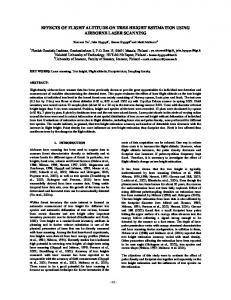
Figure 1. For Elliot Ranch, each sample plot’s relative height (top height divided by maximum observed height) is plotted over selection by percentile at growing stock levels (40 –160) for selection by height (a), selection by dbh (b), and selection by dbh2 ⴛ height (c).
Figure 3. For Crawford Creek, each sample plot’s relative height (top height divided by maximum observed tree height) is plotted over selection by percentile at growing stock levels (30 –140) for selection by height (a), selection by dbh (b), and selection by dbh2 ⴛ height (c).
Figure 2. For Elliot Ranch, each sample plot’s relative height (top height divided by maximum observed height) is plotted over selection by trees per acre by growing stock levels (40 –160) for selection by height (a), selection by dbh (b), and selection by dbh2 ⴛ height (c).
Figure 4. For Crawford Creek, each sample plot’s relative height (top height divided by maximum observed tree height) is plotted over selection by trees per acre by growing stock levels (30 –140) for selection by height (a), selection by dbh (b), and selection by dbh2 ⴛ height (c).
Results and Discussion
height and drive down estimates of site index derived from this top height. This is confirmed in the plots of relative height (Figures 1– 4), where the steepest part of the curve is usually at the lowest
It is axiomatic that the more trees selected from a sorted list (largest to smallest) will produce progressively lower estimates of top
WEST. J. APPL. FOR. 27(1) 2012
21
levels of selection (fewer than 20 trees per acre or the 10th percentile). In Figures 1– 4, a flat line is indicative of a lack of sensitivity to selection intensity, whereas a steep or erratic trend suggests that small changes in the number or percentage of tree selected may have a great impact on resulting top height and site index estimates. Stability of any top height metric with regard to the number of trees selected is a desirable feature, as it implies robustness in a derived site index estimate. At Crawford Creek, selecting by percentile produced fairly steep slopes (Figure 3), although this trend was less pronounced at Elliot Ranch (Figure 1). These curves tend to be steeper for percentile selection at the highest densities because when selecting by percentile from a dense plot, a small change in percentile selected involves a greater number of trees than the same percentile from a more open stand. By the same token, in the more open stands, the same change in percentile selected represents fewer trees and has less influence on top height. The relationship between top height and trees per acre or percentile selected by the tallest trees is monotonic (e.g., Figure 1a), whereas section by dbh or dbh2ht can produce erratic trends, particularly at the low selection intensity levels (e.g., Figure 1b and 1c). Tables 4 and 5 present the results of linear fits over GSL. The probability levels (P values) test the hypothesis that the slope of the line relating top height to GSL is zero. Thus a significant probability level is evidence of some degree of top-height instability across varying levels of density, using an assumed linear relationship. The actual magnitude of the slope is expressed as a value labeled ⌬, which is the estimated change in top height (ft) associated with an increase in density of 100 GSL. This ⌬ value is just below the maximum observed effect on top height conditioned on the range in values of this study. Fits for top height at Elliot Ranch presented in Table 4 reveal a reduction in top height of approximately 4.4 ft for an increase in GSL of 100 when top height is defined as the 10 tallest trees per acre. However with a P value of 0.08, this is of marginal statistical significance. In general, selecting by trees per acre at Elliot Ranch appears to provide top height estimates that are fairly stable across a range of densities. Changes in top height for a change of 100 GSL range from ⫺4.4 to ⫹3.3 ft within a range of the tallest 10 to tallest 60 trees per acre, and none of these are significant departures from zero at the 5% level. Similarly, selecting by largest diameter trees per acre at Elliot Ranch shows a range of GSL effects from ⫺4.0 ft to 2.6 ft, and again, none of these values is statistically different from zero at the 5% level. In contrast, selection by a proportion of the distribution of heights at Elliot Ranch results in top height values that change more with density (ranging from ⫺8.6 to ⫺13.8 ft when selecting by height), and these values are all highly significant (all P values ⬍0.01). Selecting by a proportion of dbh or dbh2ht produces similar results. The tradeoff is in the intercept value (I-40 is the intercept translated to top height at a minimum GSL of 40). In other words, for any given level of density, the top height values are less sensitive to proportional selection than selection by trees per acre. So if top height of the most open stands is considered a true achievable top height, then there is a distinct tradeoff between selection by proportion and selection by trees per acre. At Crawford Creek, the general trends are the same, although top height values are much lower. However, the range of top height values for selection by trees per acre trends more strongly negative (a greater effect of increasing density on decreasing top height). The range of values here is ⫺4.2 ft to ⫺8.1 ft, and one must also consider 22
WEST. J. APPL. FOR. 27(1) 2012
Table 4. Elliot Ranch results for fit of top height as a linear function of growing stock level (GSL) for combinations of number of trees per acre (TPA) or percentile where the selection is based on height, dbh, and dbh2 ⴛ height (dbh2ht). The intercept is the mean top height for the lowest GSL (I-40), and the slope is expressed as a change in top height associated with a change of 100 GSL. Selection Largest TPA by height 10 20 30 40 50 60 Largest TPA by dbh 10 20 30 40 50 60 Largest TPA by dbh2ht 10 20 30 40 50 60 Percentile by height 95th 90th 85th 80th 75th 70th Percentile by dbh 95th 90th 85th 80th 75th 70th Percentile by dbh2ht 95th 90th 85th 80th 75th 70th
I-40
⌬GSL ⫽ 100
P value
135.0 129.2 123.4 122.3 117.2 114.2
⫺4.41 ⫺2.78 0.33 ⫺0.96 2.31 3.29
0.084 0.308 0.925 0.829 0.711 0.598
130.8 128.3 123.9 122.4 117.5 114.9
⫺4.03 ⫺4.85 ⫺2.92 ⫺2.54 1.17 2.57
0.134 0.095 0.438 0.533 0.858 0.696
132.9 128.6 123.8 122.2 118.7 115.2
⫺5.05 ⫺3.99 ⫺0.19 ⫺0.19 0.10 2.44
0.067 0.177 0.617 0.635 0.988 0.717
139.9 139.1 138.5 137.5 136.7 135.8
⫺8.64 ⫺10.6 ⫺12.2 ⫺12.8 ⫺13.4 ⫺13.8
0.009 0.001 0.000 0.000 0.000 0.000
133.7 131.6 132.7 132.2 131.7 131.5
⫺6.47 ⫺6.79 ⫺9.14 ⫺10.0 ⫺10.7 ⫺11.6
0.089 0.075 0.017 0.009 0.006 0.002
136.8 136.7 136.3 135.3 134.2 132.9
⫺8.22 ⫺10.9 ⫺11.9 ⫺12.5 ⫺12.2 ⫺12.0
0.025 0.003 0.001 0.001 0.001 0.001
that because Crawford Creek is a less productive site, these top height responses as a proportion of total height are greater than those observed at Elliot Ranch. As the number of trees selected for top height estimation increases, the probability levels tend to increase using trees per acre on both sites. As long as enough trees are selected (about the 20 largest per acre), one would expect top height values to be fairly robust for a wide range of density values on a good site such as Elliot Ranch, and perhaps less so for a poorer site such as Crawford Creek. When trees are selected using a proportion of the distribution, density is generally highly statistically significant, and the estimate of ⌬ is large relative to that observed when selection is by trees per acre (Table 4). The difference in sensitivity to selection method between the two sites appears to be a result of a greater range of heights for any given definition of dominance at Elliot Ranch, because thinnings were executed from below at both sites. It should be noted that sensitivity to changing the number of the largest trees per acre defining top height was high at Elliot Ranch
Table 5. Crawford Creek results for fit of top height as a linear function of growing stock level (GSL) for combinations of number of trees per acre (TPA) or percentile where the selection is based on height, dbh, and dbh2 ⴛ height (dbh2ht). The intercept is the mean top height for the lowest GSL (I-30), and the slope is expressed as a change in top height associated with a change of 100 GSL. Selection Largest TPA by height 10 20 30 40 50 60 Largest TPA by dbh 10 20 30 40 50 60 Largest TPA by dbh2ht 10 20 30 40 50 60 Percentile by height 95th 90th 85th 80th 75th 70th Percentile by dbh 95th 90th 85th 80th 75th 70th Percentile by dbh2ht 95th 90th 85th 80th 75th 70th
I-30
⌬GSL ⫽ 100
P value
83.4 79.8 77.3 78.2 76.6 75.2
⫺5.27 ⫺5.12 ⫺4.23 ⫺6.98 ⫺6.44 ⫺6.03
0.059 0.067 0.129 0.079 0.104 0.128
80.3 77.7 77.3 76.7 75.5 74.4
⫺6.37 ⫺5.42 ⫺6.35 ⫺8.06 ⫺7.47 ⫺7.36
0.025 0.055 0.025 0.045 0.062 0.067
80.4 77.8 76.7 77.2 76.0 74.5
⫺5.13 ⫺5.43 ⫺5.45 ⫺7.36 ⫺6.98 ⫺6.51
0.065 0.051 0.050 0.062 0.077 0.099
84.5 83.5 82.7 82.4 81.5 81.0
⫺9.09 ⫺10.6 ⫺11.6 ⫺12.7 ⫺13.1 ⫺13.7
0.004 0.000 0.000 0.000 0.000 0.000
81.5 80.7 79.9 79.7 78.6 77.9
⫺8.99 ⫺10.5 ⫺11.1 ⫺12.0 ⫺11.9 ⫺12.3
0.005 0.001 0.001 0.000 0.000 0.000
82.6 81.2 81.0 80.5 80.0 79.7
⫺8.99 ⫺9.92 ⫺11.1 ⫺12.1 ⫺12.8 ⫺13.4
0.006 0.002 0.000 0.000 0.000 0.000
and relatively low at Crawford Creek. At Elliot Ranch, the more productive of the two sites, there was greater within-plot variability in tree heights among the larger trees. SD of height of the 40 tallest trees per acre, for example, was consistently higher for Elliot Ranch than Crawford Creek. If resulting estimates of site index are indeed affected by density management, then what effect might this have on management? First, if site index is being used to drive growth models, it may lead to underestimated height growth and volume response to density management. The degree is difficult to determine, as it will depend on the particular growth models and the linkages between diameter and height growth. Second, it is possible to underestimate the value of unmanaged stands, as the true potential site index may be higher than that observed. In comparing two ponderosa pine stands with the same estimated site index, one with density management and one without, the unmanaged stand will have the greater capacity for productivity as indexed by height, because site index is effectively underestimated in the unmanaged stand.
Finally, although there are no standards for the way in which top height is defined, we find that the definition itself may overwhelm any concerns for the effects of density. For example, a site index value derived from a definition of the largest 10 trees per acre is not comparable to one derived from the largest 40 trees per acre. Therefore, a consistent definition for top height in ponderosa pine is important for comparable site index estimates.
Conclusions In general, we found that top height in ponderosa pine decreased with increasing stand density. If resilience to changes in density is desired, then selection by trees per acre rather than percentile should be favored. At the most productive site, the effect of changes in GSL appeared to be most influential for selection by percentile whereas this trend was less pronounced at the poorer site. Similarly, with lower productivity, selection by trees per acre minimized the GSL effect on top height estimation. Selection of dominant trees by a percentile of the size distribution appeared to be sensitive to density and may be inadvisable if site index estimations are required across a range of densities. Selecting by tree height tends to produce the highest values of top height. However, it would appear that if top height is defined with a limit between the largest 20 – 40 trees per acre, the distinction between sorting by diameter, height, or basal-area-weighted height are relatively small. For comparative purposes, site index estimates should be accompanied by the specification of top height, and comparisons of ponderosa site index without a clear definition of top height should probably be avoided.
Literature Cited ALEXANDER, R.R., D. TACKLE, AND W.G. DAHMS. 1967. Site indexes for lodgepole pine, with corrections for stand density: Methodology. US For. Serv. Res. Pap. RM-29. 8 p. ARVANITIS, L.G., J. LINDQUIST, AND M. PALLEY. 1964. Site index curves for even-aged young-growth ponderosa pine of the west-side Sierra Nevada. Cal. For. Prod. No. 35. Cal. Ag. Exp. Stn. ASSMANN, E. 1970. The principles of forest yield study. Pergamon Press, Oxford. 506 p. BAKER, F.S. 1953. Stand density and growth. J. For. 51:95–97. BARRETT, J.W. 1978. Height growth and site index curves for managed even-aged stands of ponderosa pine in the Pacific Northwest. US For. Serv. Res. Pap. PNW-232. BIGING, G.S. 1985. Improved estimates of site index curves using a varying parameter model. For. Sci. 31(1):248 –259. COCHRAN, P.H., AND J.W. BARRETT. 1995. Growth and mortality of ponderosa pine poles thinned to various densities in the Blue Mountains of Oregon. US For. Serv. Res. Pap. PNW-RP-483. CURTIS, R.O., D.J. DEMARS, AND F.R. HERMAN. 1974. Which dependent variable in site index-height-age regressions? For. Sci. 20:74 – 87. DEMARS, D.J. AND J.W. BARRETT. 1987. Ponderosa pine managed-yield simulator: PPSIM Users guide. US For. Serv. Gen. Tech. Rep. PNW-GTR-203. DUNNING, D. 1942. A site classification for the mixed-conifer selection forests of the Sierra Nevada. US For. Serv. Cal. For. Range Exp. Stn. Res. Note 28. DUNNING, D. AND L.H. REINEKE. 1933. Preliminary yield tables for second-growth stands in the California pine region. US Tech. Bull. 354. 23 p. FLEWELLING, J., R. COLLIER, B. GONYEA, D. MARSHALL, AND E. TURNBLOM. 2001. Height-age curves for planted Douglas-fir, with adjustments for density. SMC Working Paper No. 1. Stand Management Coop., College of Forest Resources, Univ. of Washington. GARCIA, O. 1998. Estimating top height with variable plot sizes. Can. J. For. Res. 28:1509 –1517. GARCIA, O. 2005. Top height estimation in lodgepole pine sample plots. West. J. Appl. For. 20:64 – 68. HANN, D.W. 2009. ORGANON user’s manual, ed. 8.4. Department of Forest Resources, Oregon State Univ., Corvallis, OR. 129 p. HANN, D.W., AND J. SCRIVANI. 1987. Dominant-height-growth and site-index equations for Douglas-fir and ponderosa pine in southwest Oregon. Oregon State Univ. For. Res. Lab. Res. Bull. 59. WEST. J. APPL. FOR. 27(1) 2012
23
KING, J.E. 1966. Site index curves for Douglas-fir in the Pacific northwest. Forestry Paper 8. Weyerhaeuser For. Res. Center. LYNCH, D. 1958. Effects of stocking on site measurement and yield of second-growth ponderosa pine. US For. Serv. Intermountain For. Range Exp. Stn. Res. Pap. 56. MAILLY, D., S. TURBIS, I. AUGER, AND D. POTHIER. 2004. The influence of site tree selection method on site index determination and yield prediction in black spruce stands in northeastern Que´bec. For. Chron. 80:134 –140. MAGNUSSEN, S. 1999. Effect of plot size on estimates of top height in Douglas-fir. West. J. Appl. For. 14:17–27. MEYER, W.H. 1938. Yield of even-aged stands of ponderosa pine. US Tech. Bull. 630. 59 p. MYERS, C.A. 1967. Growing stock levels in even-aged ponderosa pine. US Forest Service Res. Pap. RM-33. 8 p. MILNER, K.S. 1992. Site index and height growth curves for ponderosa pine, western larch, lodgepole pine, and Douglas-fir in western Montana. West. J. Appl. For. 7:9 –14. MINOR, C.D. 1964. Site index curves for young-growth ponderosa pine in northern Arizona. US For. Serv. Res. Note RM-37. OLIVER, W.W. 1997. Twenty-five-year growth and mortality of planted ponderosa pine repeatedly thinned to different stand densities in northern California. West. J. Appl. For. 12(4):122–130.
24
WEST. J. APPL. FOR. 27(1) 2012
OLIVER, W.W. 2005. The West-wide ponderosa pine levels-of-growing-stock study at age 40. In Proc. of the symp. on ponderosa pine: Issues, trends and management, Ritchie, M.W., D.A. Maguire, and A. Youngblood (tech. coords.). US For. Serv. Gen. Tech. Rep. PSW-GTR-198. PERACCA, G.G., AND K.L. O’HARA. 2008. Effects of growing space on growth for 20-year old giant sequoia, ponderosa pine and Douglas-fir in the Sierra Nevada. West. J. Appl. For. 23:156 –165. PIENAAR, L.V., AND B.D. SHIVER. 1984. The effect of planting density on dominant height in unthinned slash pine plantations. For. Sci. 30:1059 –1066. POWERS, R.F. 1972. Estimating site index of ponderosa pine in northern California: standard curves, soil series, stem analysis. US For. Serv. Res. Note PSW-265. POWERS, R.F., AND W.W. OLIVER. 1978. Site classification of ponderosa pine stands under stocking control. US For. Serv. Res. Pap. PSW-128. REINEKE, L.H. 1933. Perfecting a stand-density index for even-aged forests. J. Ag. Res. 46:627– 638. RENNOLLS, K. 1978. “Top Height”; its definition and estimation. Commonw. For. Rev. 57:215–219. RITCHIE, M.W., AND D.W. HANN. 1990. Equations for predicting the 5-year height growth of six conifers species in southwest Oregon. Res. Pap. 54. Oregon State Univ. Forest Res. Lab. SHARMA, M., R.L. AMATEIS, AND H.E. BURKHART. 2002. Top height definition and its effect on site determination in thinned and unthinned loblolly pine plantations. For. Ecol. Manag. 168:163–175.