Efficiencies of Different Genes and Different Tree-building in Recovering a Known Vertebrate Phylogeny Claudia A. M. RUSSO,~Naoko Takezaki, and Masatoshi Institute of Molecular
Evolutionary
Genetics
and Department
Methods
Nei
of Biology, Pennsylvania
State University
The relative efficiencies of different protein-coding genes of the mitochondrial genome and different tree-building methods in recovering a known vertebrate phylogeny (two whale species, cow, rat, mouse, opossum, chicken, frog, and three bony fish species) was evaluated. The tree-building methods examined were the neighbor joining (NJ), minimum evolution (ME), maximum parsimony (MP), and maximum likelihood (ML), and both nucleotide sequences and deduced amino acid sequences were analyzed. Generally speaking, amino acid sequences were better than nucleotide sequences in obtaining the true tree (topology) or trees close to the true tree. However, when only first and second codon positions data were used, nucleotide sequences produced reasonably good trees. Among the 13 genes examined, Nd5 produced the true tree in all tree-building methods or algorithms for both amino acid and nucleotide sequence data. Genes Cytb and Nd4 also produced the correct tree in most tree-building algorithms when amino acid sequence data were used. By contrast, Co2, ZVdl, and Nd4Z showed a poor performance. In general, large genes produced better results, and when the entire set of genes was used, all tree-building methods generated the true tree. In each tree-building method, several distance measures or algorithms were used, but all these distance measures or algorithms produced essentially the same results. The ME method, in which many different topologies are examined, was no better than the NJ method, which generates a single final tree. Similarly, an ML method, in which many topologies are examined, was no better than the ML star decomposition algorithm that generates a single final tree. In ML the best substitution model chosen by using the Akaike information criterion produced no better results than simpler substitution models. These results question the utility of the currently used optimization principles in phylogenetic construction. Relatively simple methods such as the NJ and ML star decomposition algorithms seem to produce as good results as those obtained by more sophisticated methods. The efficiencies of the NJ, ME, MP and ML methods in obtaining the correct tree were nearly the same when amino acid sequence data were used. The most important factor in constructing reliable phylogenetic trees seems to be the number of amino acids or nucleotides used.
Introduction It is well known that the phylogenetic trees reconstructed from different genes for the same set of organisms are often different (e.g., Goodman et al. 1982; Hedges 1994). This is true even with mitochondrial DNA (mtDNA), where all genes are inherited together without recombination and there is no confusion of orthologous and paralogous genes (e.g., Cao, Adachi, and Hasegawa 1994; Cao et al. 1994; Simon et al. 1994; Honeycutt et al. 1995). The differences between phylogenetic trees reconstructed may be caused by sampling error of nucleotides or codons, different patterns of nucleotide or amino acid substitutions, etc., but in most cases it is difficult to know which of the reconstructed trees is the correct one because the true tree is unknown. It is possible that some genes are more suitable for re‘Present address: Departamento eral do Rio de Janeiro, Brazil.
de Genetica,
Universidade
Fed-
Key words: mtDNA genes, neighbor joining, minimum evolution, maximum parsimony, maximum likelihood, vertebrate species, molecular phylogeny. Address for correspondence and reprints: Masatoshi Nei, Institute of Molecular Evolutionary Genetics and Department of Biology, 328 Mueller Laboratory, The Pennsylvania State University, University Park, Pennsylvania 16802. Email:
[email protected]. Mol. Biol. Evol. 13(3):525-536. 1996 0 1996 by the Society for Molecular Biology and Evolution. ISSN: 0737-4038
constructing a phylogenetic tree than others, but it is usually difficult to know which gene is the best. This problem can be solved if the true phylogeny of the organisms is known. Hillis, Huelsenback, and Cunningham (1994) studied the accuracy of a reconstructed tree by producing an artificially generated phylogeny in phages, inducing mutation by chemical mutagens. While this experiment is interesting, it is desirable to examine the accuracy of the trees reconstructed by using existing organisms. Actually, there are organisms of which the phylogeny is firmly established by fossil records and morphological characters. For example, no one would dispute the phylogenetic relationships of humans, chimpanzees, macaques, marsupials, birds, and bony fishes. If we use these groups of organisms, it is possible to determine how reliable a particular gene is for obtaining the correct tree. One of the purposes of this paper is to study this problem by using 13 protein-coding genes in the mitochondrial genome for a group of vertebrate species, of which the phylogeny is known. Because the number of codons and the extent of sequence divergence differ considerably among the genes, it is possible to examine their effects on the phylogenetic tree reconstructed. In this paper we are also interested in studying the effi525
526
Russo et al.
Rat
loo
la,
Bibb et al. 1981), rat (Rattus norvegicus-X14848, Gadaleta et al. 1989), opossum (Didelphis virginiana229573, Janke et al. 1994), chicken (Gallus gallusX52392, Desjardins and Morais 1990), African clawed M 102 17, X0 1600, and frog (Xenopus Zaevis-X02890, X01601, Roe et al. 1985), rainbow trout (Oncorhynchus mykiss-L2977 1, R. Zardoya, J. M. Bautista, and A. Garrido-Pertierra, unpublished data), loach (Crossostoma Zacustre-M9 1245, Tzeng et al. 1992), and carp (Cyprinus carpio-X6 10 10, Chang, Huang, and Lo 1994). The phylogenetic tree of these organisms is known (Car-i-01 1988, pp. 11,605-606; Gingerich, Smith, and Simons 1990; Gingerich et al. 1994) and is given in figure 1. The nucleotide sequences were retrieved from the GenBank, except the carp sequence, which was taken from the EMBL databank. Protein-coding nucleotide sequences were converted into amino acid sequences according to the mammalian mitochondrial genetic code. The amino acid sequences for two subunits of adenosine triphosphatase (genes Atp6 and Atp8), cytochrome b (Cytb), three subunits of cytochrome c oxidase (Cal, Co2, and Co3), and seven subunits of nicotinamide adenine dinucleotide dehydrogenase (Ndl, Nd2, Nd3, Nd4, Nd41, Nd5, and Nd6) were then aligned for each protein separately by using the CLUSTAL V computer program (Higgins, Bleasby, and Fuchs 1992) with the default option. All sites with alignment gaps were removed from data analysis. The numbers of codons used for each gene and the entire set of 13 genes are given in table 1. In the analysis of DNA sequences, we used the nucleotide sequences of each gene determined by the alignment of amino acid sequences. Therefore, the number of nucleotides for each gene is three times the number of codons. In this study the nucleotide sequences for rRNAs, tRNAs, control region, and intergenic regions were not used.
Moose
100
OpoJsm
la,
ChidLm
xmopvJ Trout LWCh Carp I
0
I
0.05
FIG. l.-The known tree used in this paper. The phylogenetic relationships of the 11 vertebrate species are based on morphological characters and fossil records. The branch lengths are least-squares estimates of the neighbor-joining tree with Poisson-correction distance. p: Balaenoptera physalus. m: B. muse&s.
ciencies of different tree-building methods or algorithms in recovering the correct tree, though this scope is somewhat limited because there are only 13 genes. Our primary interest is in the trees constructed from amino acid sequences, as the organisms used are distantly related and synonymous substitutions are apparently saturated (Cao et al. 1994). However, we will also examine phylogenetic trees constructed from DNA sequences for the sake of comparison with protein sequence trees. Materials Organisms
and Methods and Sequence
Data
There are now many complete mtDNA sequences from diverse groups of organisms. For our study, we have chosen sequences from 11 vertebrate organisms for which the evolutionary relationships are established and the complete sequence is available. The organisms used (and the source of the sequences with the GenBank accession numbers) are two whale species (Balaenoptera physalus-X61145, Amason, Gullberg, and Widegren 199 1; Balaenoptera musculus-X72204, Arnason and Gullberg 1993), cow (Bos taurus-VO0654 and 501394, Anderson et al. 1982), mouse (Mus musculus-V00711, Table 1 Some Statistical Genes
Properties
of 13 Mitochondrial
Atp6
Number of codons . . . . . . . 219 5 Minimum p distance (%) . . Maximum p distance (%) . . 50 2.1 Gamma parameter . . . . . . . . Parsimony sites* . . . . . . . . . 119 RCI (%)t . . . . . . . . . . . . . . . 71
Atp8 52 10 79 13.3 44 73
Co1 511 1 14 0.5 81 55
Phylogenetic
Analysis
To reconstruct phylogenetic trees from the 13 genes and the entire set of genes, we used four commonly used
Genes for Amino Acid Sequence Data
co2 224 1 33 1.6 68 72
co3 259 1 25 0.7 64 71
Cytb 377 3 28 0.9 121 54
Ndl 312 1 33 1.1 117 54
Nd2 342 5 58 3.4 207 57
Nd3 112 0 44 1.1 54 71
Nd4 457 7 60 1.7 212 59
Nd41 97 3 42 4.7 51 76
Nd5
Nd6
All
582 3 44 1.6 278 54
138 5 67 8.1 92 71
3,682$ 3 37 1.2 1,508 61
* Phylogenetically informative sites for parsimony analysis. t RCI stands for the average resealed consistency index for the reconstructed unweighted parsimony tree(s). $ There are small proportions of overlapping codons between Afp6 and A@8 and between Nd4 and Nd41, but they were treated as though they were independent codons.
Mitochondrial
tree-building methods: neighbor joining (NJ) (Saitou and Nei 1987), minimum evolution (ME) (Rzhetsky and Nei 1992), maximum parsimony (MP) (Eck and Dayhoff 1966, p. 165), and maximum likelihood (ML) (Felsenstein 198 1). Amino Acid Sequences The NJ and ME methods are so-called distance methods and require pairwise distances. For amino acid sequence data, we used three different distance measures: proportion of amino acid differences (p distance), Poisson-correction distance, and gamma distance (see MEGA; Kumar, Tamura, and Nei 1993). The gamma distance takes into account the heterogeneity of evolutionary rates among different amino acid sites, and the extent of heterogeneity is measured by the gamma parameter a. The a value was estimated by using the computer program GAMMA (S. Kumar, personal communication), which is based on parsimony analysis (Kocher and Wilson 1991). GAMMA requires an input tree, and we used the known tree in all cases. NJ trees were constructed by using MEGA, whereas ME trees were constructed by the program METREE (Rzhetsky and Nei 1994). ME trees were constructed only for p distance and Poisson-correction distance, because METREE does not compute gamma distance. In the search for ME trees, we examined only the NJ tree or trees whose topological distance (dT; see below) from the NJ tree (not the true tree) was 2 or 4, since the ME and NJ trees are known to be very similar to each other (Rzhetsky and Nei 1992). In the present case the number of trees with dT = 2 is 16, but the number of trees with dT = 4 varies with the topology of the NJ tree (Rzhetsky and Nei 1992). In the case of the true tree in figure 1 the number is 160. Maximum-parsimony trees were constructed by using the default option of the branch and bound search of the software PAUP (Swofford 1993). Both weighted and unweighted MP trees were produced. Unweighted parsimony generated a single most parsimonious tree for all genes except for Atp6, Atp8, and Cal, where 3, 3, and 2 equally parsimonious trees were produced, respectively. When two or more parsimonious trees were obtained, we constructed a strict consensus tree. Weighted parsimony was performed by using the resealed consistency index (Farris 1989) as a weighting factor for each parsimony site. This index varies from 0 (high degree of homoplasy) to 1 (no homoplasy). (Homoplasy is equivalent to parallel and backward mutations.) In this study we applied this weighting procedure only for one cycle. Weighted parsimony always produced a single most parsimonious tree. To produce ML trees, we used Adachi and Hasegawa’s (1994) program ProtML. Because the ML meth-
Genes and Tree-building
Methods
527
od for protein data requires a large amount of computer time, we first used the star decomposition (SD) algorithm, which generates one final tree, as in the case of the NJ method. This tree (SD tree) may not be the real ML tree, so we also used the specific-tree algorithm, which examines any set of specified trees. We examined all trees whose topological distance from the SD tree was equal to 2 or 4 and chose the tree showing the highest likelihood as the ML tree. This algorithm is similar to that of finding ME trees (Rzhetsky and Nei 1992). We used four different ProtML substitution models for constructing trees, i.e., the Poisson, Dayhoff, JTT, and JTT-f models. The Poisson model uses a Poisson model of amino acid substitution, whereas the Dayhoff and JTT algorithms use the empirical amino acid substitution models based on the data compiled by Dayhoff, Schwartz, and Orcutt (1978) and Jones, Taylor, and Thornton (1992), respectively. The JTT-f model uses Jones, Taylor, and Thornton’s substitution model under the assumption that the relative frequencies of the 20 different amino acids in a sequence are identical with the average observed frequencies for all sequences and remain the same for the entire evolutionary process. Actually, we also used the Poisson and Dayhoff models with the observed amino acid frequencies, but this modification hardly affected the topologies of the trees obtained. Therefore, we shall not consider these models in this paper. Nucleotide
Sequences
To compare the utility of DNA sequences for phylogenetic construction with that of amino acid sequences, we constructed phylogenetic trees for all genes by using either all three codon positions of the sequences or first and second codon positions only. In both sets of data we again used the NJ, ME, MP, and ML methods. The distance measures used for NJ were the p, JukesCantor, Kimura-2-parameter, and gamma distances (see Nei 1991). The values of gamma parameter a were also computed by using the program GAMMA. In the case of the ME method we used only the p, Jukes-Cantor, and Kimura-2-parameter distances. The NJ and ME trees were constructed by MEGA and METREE, respectively. In the case of MP trees, we again used PAUP for both unweighted and weighted parsimony. Weighting was done by using the resealed consistency index. The ML trees were constructed by using the NucML program by Adachi and Hasegawa (1994). We again used the SD algorithm and the specific-tree algorithm for trees with dT = 2 and 4. The substitution models used were the Poisson, proportional, and HKY (Hasegawa, Kishino, and Yano 1985) models (see Adachi and Hasegawa 1994).
528
Russo et al.
Table 2 Pairwise p Distances ganisms
1 2 3 4 5 6 7 8 9 10 11
Whale-p . . . . Whale-m . . . . cow . . . . . . . . Rat . . . . . . . . . Mouse . . . . . . Opossum . . . . Chicken . . . . . Xenopus . . . . Trout . . . . . . . Loach . . . . . . carp . . . . . . .
(p X 100) for Atp6 Amino Acid Sequences from 11 Vertebrate
Or-
2
3
4
5
6
7
8
9
10
11
5
23 22
29 27 23
26 25 21 5
30 30 24 28 27
45 46 44 48 47 42
48 47 45 50 49 43 31
49 47 47 49 48 44 27 20
47 46 47 48 48 45 27 25 13
48 47 49 49 48 46 27 25 12 8
NOTE.-All insertions/deletions were removed from the entire data set, and the distances were computed by using the remaining 219 amino acid sites. p, Buluenopteru physalus; m, Buluenopteru musculus. Note that mammalian species show similar distances from chicken, Xenopus, and fishes. This makes it difficult to obtain the correct tree.
Accuracy
of the Topology
Obtained
The accuracy of the tree topology obtained was measured by the topological distance of the tree obtained from the true tree. This distance (dr) is based on the work by Robinson and Foulds (198 1) and Penny and Hendy (1985) and is given by the following formula (Rzhetsky and Nei 1992). do = 2[min(q,&)
-
rl +
14r
-
%I,
where qr and qt are the total numbers of ways of sequence partitions (equal to the number of interior branches) for the tree reconstructed from a given data set and for the true tree, respectively, and r is the number of partitions (interior branches) that are identical for the two trees. For bifurcating trees, dT is equal to twice the number of sequence partitions for which the two trees compared are different (incorrect interior branches of the reconstructed tree). Thus, dT = 0 means that the tree obtained is the same as the true tree, and as dr increases, the deviation from the true tree increases. In the case of MP trees we also computed the average rescaled consistency index (RCI) for all parsimony sites to examine the reliability of the tree obtained. To compare the efficiencies of different tree-building methods, we used the sum of dr for all genes and the number of genes generating the correct topology (nc) among the 13 genes examined. Results Statistical
Properties
of Different
Genes
Table 1 shows various statistical properties of the 13 mitochondrial genes used in this study. The number of codons or amino acids encoded varies from 52 (Atp8) to 582 (Nds), and thus we can examine the effect of gene size on the accuracy of the tree reconstructed. The
minimum and maximum p distances indicate that some genes (e.g., Co1 and Co3) are highly conserved whereas others (e.g., Atp8 and N&) are quite divergent. Of course, the distance value varies with sequence pair, and table 2 shows the magnitude of variation in p among different pairs of sequences for the gene Atp6 as an example. The gamma parameter also varies from gene to gene, but the extent of heterogeneity of substitution rate (l/u) is not so great as in the case of the control region of mtDNA sequences, where a = 0.15 has been obtained (Kocher and Wilson 1991). The number of amino acid sites that are informative for parsimony analysis (parsimony sites) varies from 44 to 278, suggesting that some genes are much more useful for parsimony analysis than others. The average resealed consistency index, which is supposed to be negatively correlated to the extent of parallel or backward mutations, varies from gene to gene, but this index seems to have no correlation with the maximum p distance. Reconstruction of Phylogenetic Amino Acid Sequences
Trees
Table 3 shows the topological distances (dT) of reconstructed trees from the true tree for different genes and different tree-building methods. Gene Nd5 produced the correct tree in all tree-building methods and algorithms used, and genes Cytb and Nd4 also produced the correct tree in all the methods except in a few ML algorithms. Co3 produced the correct tree in all parsimony and ML algorithms and in the NJ and ME methods with p distance. By contrast, genes Co2, Ndl, and Nd4Z generated incorrect trees in all tree-building methods. The topologies produced by different tree-building algorithms were often the same or very similar, though there were several exceptions (Atp8, Co2, Nd3, Nd41, and Nd6). These results indicate that when a tree-building
Mitochondrial
Table 3 Topological
Distances (&) of Reconstructed
Genes
Atp6
Atp8
Co1
co2
2 2 2
2 0 0
2 0 0
2 2
2 0
2 2
Genes and Tree-building
Methods
529
Trees from the True Tree co3
Cytb
4 4 4
0 2 2
0 0
4 4
0 2
0
Ndl
Nd2
Nd3
Nd4
2 2 2
0 2 2
2 0 0
0 0
2 2
2 2
2 2
0
Nd41
Nd5
Nd6
All
Sum
n,
0
16 14 16
6 7 7
18 18
5 5
NJ P .............. Poisson ........ Gamma ........ ME P .............. Poisson ........ MP Unweighted ..... Unweighted-b ... Weighted ....... Weighted-b ..... ML star decom. Poisson ........ Dayhoff ........ JTT ........... JTT-f .......... ML specific-trees Poisson ........ Dayhoff ........ JTT ........... JTT-f .......... Sum ............
2 1 2 2
0 2 0 0
0 0 0 2
8 8 8 8
0 0 0 0
0 0 0 0 21
10 10 4 4 99
0 0 0 0 6
2 4 2 6 31
0
0 0 0
1 1 2 1
0 2 0 0 25
0
0 0
0 0
0 0 0
2 2 4
0
0
2 2 4
0 0
0 0
0
0
0
0
2 2
0
0
0
0
0
0
2 1 2 2
0
0
0
na 0 na
2 2 2 2
0
2 2 2 2 45
0 0
0 0
0 2 0 0 0 26
4 2 2 2 48
0 0 2 2 8
6 8 4 4 66
0 0
0 0 0
0 0 2 2 28
21 21 20 21 18 26 22 24
8 5 6 4
26 28 20 24
7 7 5 5
Nom.-Unweighted-b stands for unweighted bootstrap consensus trees and weighted-b weighted bootstrap consensus trees. na: Because of a large amount of computer time required, the tree was not constructed. n,: Numbers of genes that produced the true tree. The dT values in boldface letters indicate that the ML value for the tree obtained is lower than that of the true tree.
method produces a given topology other methods or algorithms also tend to produce the same topology, whether it is correct or not. This finding is similar to that observed in Saitou and Imanishi’s (1989) computer simulation with respect to DNA sequences. If the differences in dT among different tree-building methods are primarily caused by sampling error of nucleotides, one would expect that large genes tend to produce the correct tree more often than small genes. There is certainly such a tendency, but some large genes (e.g., Cal) sometimes produced incorrect trees. Therefore, there must be some other factors that affect the accuracy of the tree reconstructed. One such factor could be the pattern of amino acid substitution. If this pattern varies from gene to gene, different genes may produce different topologies. We therefore examined this pattern by estimating the transition matrix of amino acids for each gene. In this study we used Yang’s (1995) computer program PAML to estimate all the elements of the 20 X 20 transition matrix under the assumption of the general reversible amino acid substitution model. However, all genes produced very similar transition matrices. Therefore, it was difficult to explain the differences in dT by different amino acid substitution patterns. In the case of Col, however, the small extent of sequence divergence (table 1) is probably responsible for its relatively poor performance.
Among different tree-building methods, NJ tends to show small &‘s, whereas ML tends to show large &‘s. The other methods show intermediate dT values. Table 3 also includes the number of genes that produced the correct topology (nc). According to this criterion, the ML star decomposition with the Poisson model is best in topology construction and is followed by NJ with Poisson-correction distance and gamma distance. However, because the number of genes examined is small, the differences in nc are not statistically significant. Clearly, we need more genes to compare different treebuilding methods, including nuclear genes. In both NJ and ME methods, we used two or three different distance measures, but they had little effect on the topology of the tree reconstructed. One might expect that a distance measure that is proportional to the number of amino acid substitutions performs better in phylogenetic reconstruction than other distances and thus either Poisson-correction distance or gamma distance is better than p distance. However, for the reconstruction of phylogenetic trees the variance as well as the linearity of a distance measure with the number of substitutions plays an important role (Nei, Tajima, and Tateno 1983; Goldstein and Pollock 1994; Tajima and Takezaki 1994). Therefore, a simple measure such as p distance or Poisson-correction distance often shows a better perfor-
530
Russo et al.
Table 4 AIC Values for Different ML Substitution Models Atp6
co1
co2
Ndl
Nd5
Nd6
Poisson . . Dayhoff . . JTT . . . . . JTT-f . . . .
779 313 222
843 319 234
547 185 110
1,024 468 294
2,011 1,007 650
674 330 236
Nom.-The the differences
minimum AIC value was observed for JTT-f for all genes, and from this minimum are given for other models.
*
*
*
*
*
*
mance. In our case all three distance measures showed more or less the same results. It is interesting to note that in the cases of genes Co1 and Nd3 with Poisson-correction distance the NJ method identified the correct topology, whereas the ME did not. This indicates that the criterion of minimum evolution led to choosing an incorrect topology rather than to improving or keeping the NJ tree. This may have happened by chance (Rzhetsky and Nei 1992), but it seems that an optimization process such as the ME criterion does not always work well with real data (see Discussion). We have used four different algorithms to produce MP trees, but in most of the genes used the four algorithms produced essentially the same topology. This raises a question about the efficiency of weighted parsimony with the RCI. It is also interesting to note that there is virtually no correlation between RCI and dT in parsimony methods. The dT value is generally small when the number of parsimony sites is large, but the correlation between the two quantities is not very high. The four different models for the ML star decomposition algorithm produced the same tree for six genes but different trees for the others. Kishino and Hasegawa (1989, 1990) suggested that when different models produce different ML trees, the most likely tree should be chosen by using the Akaike information criterion (AIC), which is defined as -2 X (estimated log likelihood) + 2 X (number of free parameters) (Akaike 1974). The tree with the smallest AIC value is supposed to be the best. The number of free parameters in AIC is the same for the Poisson, Dayhoff, and JTT models, but the number for the JTT-f is greater than that for the others by 19, because the amino acid frequencies are estimated from data. Table 4 shows the AK values for a few genes for the four different substitution models. It is clear that AIC is smallest for the JTT-f model and largest for the Poisson model. Actually, this was the case for all genes. However, table 3 shows that JTT-f is not efficient in obtaining the correct tree and the Poisson model is slightly better. Therefore, AIC does not seem to be a good criterion to choose the correct tree at least in the
present case. However, this result might have been obtained because we used the SD algorithm, which does not examine a large number of trees. Indeed, when we computed the likelihood for the true tree, the value was higher than that of the SD tree in eight cases (dr values in boldface letters in table 3). Therefore, the inefficiency of the ML criterion observed in table 3 may be due to the inefficiency of the SD algorithm. However, when we examined all trees that are different from the SD tree by dT = 2 or 4, the dT value of the ML tree did not always decrease. Rather it increased in some genes. The nc value also remained nearly the same. Interestingly, many of the ML trees obtained were not the true tree, but all of them had a likelihood value higher than that for the true tree. These results suggest that the ML criterion may not always be very efficient in obtaining the correct topology for protein sequences. The reliability of a phylogenetic tree reconstructed is expected to increase as the number of codons used increases. To examine whether this expectation is true or not, we constructed a tree based on the entire set of genes using all statistical methods except the bootstrap consensus trees by parsimony. The bootstrap consensus trees required too much computer time to be completed in a reasonable time. As is seen from table 3, the trees obtained showed the correct topology regardless of the method used. When the bootstrap test (Felsenstein 1985) was applicable, all interior branches had a bootstrap value of lOO%, and the interior branch test (Rzhetsky and Nei 1992) gave a confidence probability of 99.9% or higher for all interior branches. This clearly supports the idea that the number of codons (or characters) used is very important for constructing a reliable phylogenetic tree. Nucleotide
Sequences
As mentioned earlier, synonymous substitutions between mammalian and nonmammalian sequences are almost certainly saturated or near saturation. Therefore, nucleotide sequences are expected to be subject to a large extent of noise. However, a number of authors (e.g., Cummings, Otto, and Wakeley 1995) have used all three codon positions of nucleotide sequences for constructing trees for distantly related organisms. Some authors have used only first and second codon positions, because these positions are less affected by synonymous substitutions than third codon positions (Cao, Adachi, and Hasegawa 1994; Cao et al. 1994). It is therefore interesting to examine the efficiencies of these approaches in obtaining the correct topology. Table 5 shows the dT values of the trees obtained for each gene for the cases of all three codon positions data and first two codon positions data (the latter in parentheses). When all codon positions are used, many
Mitochondrial
Genes and Tree-building
Methods
53 1
Table 5 Topological Distances (&) of Reconstructed Trees from the True Tree for Nucleotide Sequence Date Genes
Atp6
Atp8
co1
co2
co3
Cytb
Ndl
Nd2
Nd3
Nd4
Nd41
Nd.5
Nd6
All
Sum
II,
NJ P . . . . . . . . . . . 4(O)
2(2)
2(4)
4(2)
4(2)
O(2)
2(2)
2(2)
2(O)
O(0)
2(4)
O(0)
O(0)
O(0)
24(20)
4(5)
JC* . . . . . . . . . 4(O) Kimura . . . . . . 4(O) Gamma . . . . . 4(O) ME
2(2) 2(2) 2(2)
2(4) 2(4) 2(4)
4(2) 4(2) 4(4)
4(2) 4(2) 4(2)
2(2) 2(2) 2(2)
2(2) 2(2)
2(2) 2(2)
4(O) 4(O)
O(0) O(0)
2(4) 2(4)
O(0) O(0)
O(0) O(0)
O(0) O(0)
2(2)
2(2)
4(O)
O(2)
2(4)
O(0)
O(0)
O(0)
28(20) 28(20) 28(24)
3(5) 30) 3(4)
P ........... JC . . . . . . . . . . Kimura . . . . . . MP Unweighted .. Weighted . . . . ML star decom. Poisson . . . . . Proportion? ..
2(O) 2(O) 2(O)
2(2) 2(2) 2(2)
2(4) 2(4) 2(4)
4(2) 4(4) 4(4)
2(O) 2(O) 2(O)
2(4) 4(4) 4(4)
2(2) 2(2) 2(2)
2(2) 2(2) 2(2)
2(O) 2(O) 4(O)
O(0) 2(2) 2(2)
2(4) 2(4) 2(4)
O(0) O(0) O(0)
O(2) O(2) O(2)
O(0) O(0) O(0)
22( 22) 26(26) 28(26)
3(5) 2(4) 2(4)
4(O) 4(O)
6(4) 6(4)
6(5) 4(6)
6(3) 6(4)
4(l) 4(O)
4(2) 4(2)
2(4) 2(4)
4(O) 4(O)
2(2) 2(2)
2(O) 2(O)
2(4) 2(4)
O(0) O(0)
2(2) 2(2)
na na
44(27) 42(28)
l(4) l(5)
2(2) 4(2)
4(O) 4(O) 4(O)
4(6) z(6) O(4)
4(4) 4(4) 2(4)
2(2) 4(2) 2(2)
O(0) O(0) O(0)
2(2) 2(2) 2(2)
O(2) O(2) O(2)
2(O) 2(O) O(0)
O(2) O(0) O(0)
2(2) 2(2) 2(2)
O(0) O(0) O(0)
O(2) O(2) O(2)
O(0) O(0) O(0)
22(24) 24(22) 16(18)
5(4) 5(5) 7(6)
4(4) 4(4) 4(4)
4(6) 2(6) 2(6)
4(4) 4(2) 2(2)
2(2) 4(2) 4(2)
2(2) 2(2) 2(2)
2(2) 2(2) 2(2)
O(0) O(0) O(0)
2(2) 2(2) 2(2)
O(2) O(0) O(0)
4(2) 4(2) 4(2)
O(0) O(0) O(0)
O(4) O(2) O(2)
O(0) O(0) O(0)
26(30) 26(24) 24(24)
4(3) 4(4) 4(4)
HKY . . . . . . . 4(O) ML specific-trees Poisson . . . . . 2(O) Proportion . . . 2(O) HKY
. . . . . . . 2(O)
Non.-The dT values for all three codon positions and those for first and second positions (in parentheses) are given separately. See the footnote to table 2 for boldface letters. * JC: Jukes and Cantor’s distance. t Proportion: proportional model (Adachi and Hasegawa 1994).
genes show a higher dT value than that for amino acid sequences. This suggests that nucleotide sequences are less appropriate for constructing trees for distantly related organisms. However, Nd.5 again shows dT = 0 for all tree-building methods and algorithms. Nd4 and Nd6 also show dT = 0 or 2 for all algorithms. Actually, Nd6 performs slightly better for nucleotide sequences than for amino acid sequences, but this is exceptional. The dT values for first and second codon positions data are generally slightly smaller than those for all three positions data as expected, but they are still generally higher than the values for amino acid sequence data. Some genes such as Atp6 and Nd3 tend to show a smaller dT value for this case than for the case of amino acid sequences. Table 5 shows that when all three codon positions are used the MP method shows high dT and low nc values, whereas the ML star decomposition algorithm tends to have low dT and relatively high ~2~ values. In the present case the difference between nc = 1 and nc = 7 is significant at the 5% level if we use Fisher’s exact test. Therefore, the ML star decomposition algorithm is significantly better than the MP method in obtaining the correct tree. It seems that MP is affected by substitution noise more strongly than the other methods. However, when only first and second codon positions are used, all tree-building methods show similar dT and
IZ~ values, and thus all methods seem to be equally efficient. As in the case of amino acid sequences, the efficiencies of NJ and ME in obtaining the correct tree does not improve by using distance measures that are supposed to reflect the number of nucleotide substitutions better than p distance. Similarly, in ML a more sophisticated model does not necessarily give the correct tree more often than the others. In the present set of data the HKY model showed the lowest AIC value among the three models for all genes (data not shown). The HKY model has some tendency to generate a better tree particularly in the case of the SD algorithm. However, the merit of this model is small and could be due to chance. The ME method examined about 180 trees in addition to the NJ tree. However, this algorithm has hardly affected the final tree chosen. In other words, the NJ and ME trees were the same in most cases. In the case of ML, the specific-tree algorithm examined a large number of trees including the true tree in most cases, but the performance of the algorithm in terms of dT and nc was also no better than that of the SD algorithm. Actually, the former algorithm chose an incorrect tree slightly more often than the latter, and the incorrect tree chosen always had a higher likelihood value than the true tree. As in the case of amino acid sequence data, when all 13 genes were used, the correct tree was obtained in
532
Russo et al.
all cases examined. However, the bootstrap value was about 70% for one branch of the NJ trees when all three codon-positions data were used, though the CP value was 99.9% or higher. (No bootstrap tests were done for the ME, MP, and ML methods.) Discussion Comparison
of Genes
As mentioned earlier, one of the purposes of this paper is to find mitochondrial genes that are suitable for constructing phylogenetic trees for distantly related organisms. Our results have shown that amino acid sequences are generally more informative than nucleotide sequences for constructing reliable trees and that Nd5 is the most appropriate gene for this purpose. The next best genes are Nd4 and Cytb. Actually, Nd5 seems to be most appropriate even for nucleotide sequences. By contrast, genes Co2, Ndl, and Nd4Z seem to be least appropriate. This conclusion is consistent with the results obtained by Cao et al. (1994), though their purpose was not to find appropriate genes. These authors conducted ML analysis of protein sequences to study the phylogenetic relationships of cow, fin whale, harbor seal, human, mouse, and rat. Genes Cytb, Nd4, and Nd5 produced the same tree as the genome tree obtained by using all genes, whereas Co2, Ndl, and Nd4Z did not. This result did not change when blue whale and gray seal were added (Cao, Adachi, and Hasegawa 1994). However, note that in this case the true tree is not well established (Novacek 1992), and thus this conclusion is dependent on the assumption that the genome tree is identical with the true tree. In the past Cal, Co2, and Cytb have been used extensively for phylogenetic analyses (e.g., Adkins and Honeycutt 1994; Cantatore et al. 1994), but Nd4 and Nd5 have not. Both Nd4 and Nd.5 are large genes, and their protein sequence divergences seem to be appropriate for constructing trees for distantly related organisms of higher vertebrates. We therefore recommend that these genes should be used more often. Comparison
of Models
and Algorithms
We have seen that in the cases of the NJ and ME methods Poisson-correction and gamma distances, which are supposed to reflect the number of amino acid substitutions better than p distance, are no better than the latter distance in producing the correct topology. This seems to be strange. Using computer simulation, however, Saitou and Nei (1987), Sourdis and Krimbas (1987), Saitou and Imanishi (1989), and Nei (1991) have shown that in the case of DNA sequence data p distance produces the correct tree slightly more often than the Jukes-Cantor distance, unless the rate of nucleotide substitution varies considerably with evolutionary lineage
and sequence divergence is high. This is partly because p distance has a smaller variance relative to the mean than corrected distances. Similar results were obtained by Schiiniger and von Haeseler (1993) and Tajima and Takezaki ( 1994). Figure 1 shows that the sequences from the three fish species evolved considerably slower than the others. These three species formed one cluster outside the other sequences, and all mammalian sequences evolved nearly at the same rate. Furthermore, if we impose an artificial root in the middle of the branch between mammals and nonmammals, the tree looks like a linear tree with a molecular clock. This may have helped p distance to generate trees as good as those obtained by Poissoncorrection or gamma distance. A somewhat similar statement can be made about the weighted and unweighted parsimony methods used. For the present data set, both methods showed essentially the same efficiency of obtaining the correct topology, though weighted parsimony is supposed to be better than unweighted parsimony. These results are somewhat different from those of Hillis, Huelsenback, and Cunningham (1994), Tateno, Takezaki, and Nei (1994), Huelsenbeck (1995), and Nei, Takezaki, and Sitnikova (1995), who have shown that in the case of nucleotide sequence data weighted parsimony is often more efficient than unweighted parsimony in obtaining correct topologies. One possible reason for this difference is that in our data set the extent of sequence divergence was not very large (tables 1 and 2) and in this case weighting does not give much advantage. In the case of likelihood methods we already indicated that the improvement of the substitution model in terms of the AIC value does not necessarily increase the chance of obtaining a better topology. Similar results have been obtained by Cao, Adachi, and Hasegawa (1994), Cao et al. (1994), and Yang, Goldman, and Friday (1994). These results are somewhat unexpected, because the differences in AIC among different substitution models are substantial. Using computer simulation, however, Gaut and Lewis (1995) showed that unless the extent of sequence divergence is very large the probability of obtaining the correct topology for a less complicated substitution model is essentially the same as that for a more complicated one even if sequence data are generated by the latter model. Yang (1996) also showed that a simple model (Jukes-Cantor model) may give a higher probability of obtaining the correct topology than a sophisticated model (substitution rate varying among different sites) (depending on the model tree used) even when sequence data are generated by the latter model. These studies were done with nucleotide sequence data, but the same conclusion is expected to hold with amino acid sequence data as well. However,
Mitochondrial
conducting a computer simulation with the Huelsenbeck (1995) type trees of two very long branches and two very short branches, Hasegawa and Fujiwara (1993) produced examples in which the Dayhoff model recovers the correct tree more often than the Poisson and proportional models when amino acid sequences are generated by the Dayhoff model. Therefore, if the rate of substitution varies extensively with evolutionary lineage, the above conclusion may not apply. So far we emphasized the effectiveness of simple distance measures or simple substitution models in obtaining correct topologies. However, for estimating branch lengths or evolutionary times between sequences, unbiased distances (unbiased estimators of substitutions) or correct substitution models generally give better results (Tateno, Takezaki, and Nei 1994). That is, a distance measure or substitution model that is appropriate for estimating branch lengths is not necessarily good for topology inference. In this case one can use different distance measures or substitution models for topology construction and branch length estimation (Nei, Tajima, and Tateno 1983; Nei and Takezaki 1994). For a data set similar to the present one, however, it is still advisable to use corrected distances or appropriate substitution models, because they would give more reliable branch length estimates though they may not improve topology construction. Optimization Principle in Phylogenetic Analysis In the present set of data, ME was no better than NJ in obtaining the correct topology. This is somewhat counterintuitive, because Rzhetsky and Nei (1993) have shown that the true topology has the smallest expected value of the sum of branch lengths when unbiased distances are used and this has been the theoretical basis of the ME method. In practice, however, distance estimates are subject to sampling error, and for this reason the ME method is not necessarily better than the NJ method. The criterion of maximum likelihood also does not always choose the correct topology. In fact, the ML specific-tree algorithm used here showed a tendency to be inferior to the ML star decomposition algorithm. This is partly due to sampling error, because the difference in likelihood value between the ML tree and the true tree was not statistically significant in most cases when the topologies of the two trees were different and the differences were tested by Kishino and Hasegawa’s (1989) method. However, there seem to be some other factors that make the topology estimation by likelihood complicated. At the present time, the theoretical basis of likelihood method of topology estimation remains unclear (Nei 1987, p. 324-325; Yang 1994, 1996; Yang, Goldman, and Friday 1995), and there seems to be no
Genes and Tree-building a
X 0.1
b
0.1
p
0.5
d
MP
NJ
No.
c
533
0.05
Model tree
nucl.
0.5
Methods
ha
JC
K2P
UW
W
50
92
58
55
18
89
51
100
97
65
61
89
98
56
200
100
76
72
98
99
66
300
100
82
78
99
100
72
400
100
87
83
100
100
76
500
100
91
85
100
100
79
1000
100
97
94
100
100
91
2000
100
99
99
100
100
97
FIG. 2.-Percent probabilities of obtaining the correct topology estimated by computer simulation. The model tree used is somewhat similar to that of Yang (1996) and consists of four nucleotide sequences (a, b, c, and d). The value for each branch is the expected number of nucleotide substitutions per site, and a set of four sequences was generated by using pseudorandom numbers following the model tree (see Nei, Takezaki, and Sitnikova 1995). These sequences were then used to construct a tree by the NJ, MP, and ML methods. This was replicated 1,000 times, and the proportion of cases in which the correct topology was obtained (probability of obtaining the correct topology) was computed. p, JC, and K2P stand for the p, Jukes-Cantor, and Kimura-2-parameter (not modified Kimura) distances, respectively. Nucleotide substitution was simulated by using the K2P model of a transition/transversion rate ratio equal to 2. Weighted parsimony trees were constructed following Nei, Takezaki, and Sitnikova (1995). UW unweighted parsimony. W weighted parsimony.
mathematical proof that the correct topology gives the highest expected likelihood value among all possible topologies, as will be discussed below. Comparison of Digerent Tree-building Methods It is a difficult and tricky problem to compare the relative efficiencies of different tree-building methods in obtaining correct topologies, because the theoretical basis of each method is not well established. Recently Edwards (1995) stated that in the study of evolution, which is an “after-trial” evaluation, the ML method is known to be the best. However, it should be noted that the topology estimation in phylogenetic analysis is not the same as the estimation of parameters in the classical theory of the ML method, because the maximization of likelihood is conducted separately for different topologies (different probability spaces) (Nei 1987, p. 323325; Yang 1994, 1996). Indeed, it is not difficult to construct examples in which the ML method is inferior to the MP and NJ methods (Yang 1996; N. Takezaki and M. Nei, unpublished). Figure 2 shows one such example. Of course, a series of computer simulations have shown that ML is generally slightly better than other methods in many different situations (Saitou and Im-
534
Russo et al.
anishi 1989; Fukami-Kobayashi and Tateno 1991; Hasegawa and Fujiwara 1993; Tateno, Takezaki, and Nei 1994; Kuhner and Felsenstein 1994; Huelsenbeck 1995), but still we do not know the general property of this method (Yang 1996). If the results in table 3 give any guidance, simple methods such as the NJ and the ML star decomposition algorithms give as good results as the more time-consuming ME, MP, and ML methods. This is an important finding in this paper. However, the latter methods have one advantage over the simple methods. That is, they give several alternative trees, and thus one can evaluate statistical significance between different topologies and identify a group of potentially correct trees (e.g., Kishino and Hasegawa 1989; Rzhetsky and Nei 1992). The present study has another important message; if a large gene or a good-behaving gene is used, it produces a good tree whichever method is used. It is particularly impressive that all tree-building methods produced the correct tree when the entire set of genes was used. Note that it is not necessarily easy to obtain the correct tree in the present case, because mammalian species show similar distance values from chicken, Xenopus, and fishes (table 2). At any rate, the choice of a good gene or a large number of amino acids or nucleotides seems to be more important than a choice of a particular tree-building method as long as the method has some theoretical justification. Amino Acid vs. Nucleotide
Sequences
Examining the efficiencies of protein-coding genes in estimating the topology of the genome tree for mtDNA, Cummings, Otto, and Wakeley (1995) concluded that the topology of the tree produced by a gene is a poor indicator of the topology of the genome tree. This conclusion is different from ours, and there are two reasons for this. First, it is still unclear whether their genome tree represents the true phylogenetic tree of the organisms used (whale, cow, seal, human, mouse, rat, frog, carp, and loach) (Novacek 1992), though recent molecular data tend to support it. If the genome tree is not the correct one, their conclusion is not very meaningful. Second, they used all three codon positions of nucleotide sequences and did not attempt to enhance the efficiency of any of the tree-building methods used (NJ, MP, and ML). Probably for these reasons, individual genes did not produce the genome tree (supposed to be the true tree) as often as in our data analysis. If they had used first and second codon positions only instead of all the three positions, they might have obtained better results. Data Set Used However, it should be mentioned obtained in this paper are dependent
that the results on the data set
used. As mentioned earlier, the unrooted version of the tree in figure 1 roughly satisfies the condition of a linear tree with a molecular clock, and probably for this reason we obtained the true tree when we used large genes or the entire set of genes. Actually, if several groups of fast-evolving sequences and slowly evolving sequences are mixed in the true tree, construction of the correct topology usually becomes more difficult, though theoretically all the methods used here are supposed to take care of varying substitution rates. For example, if lamprey and sea urchin sequences, which have evolved much faster than fish and Xenopus sequences, are included in our data set, we obtain an incorrect tree for all tree-building methods even if we use the entire set of genes. In this case the cluster of lamprey and sea urchin is attached to the interior branch connecting mammals and nonmammals and this branching pattern is statistically significant (data not shown). At the present time we do not know the real reason for this, but it suggests that we must be very careful about the tree obtained when many fast-evolving and slowly evolving sequences are mixed. We are now investigating this problem from a theoretical point of view. Acknowledgments We thank Sudhir Kumar for his help in the alignment of sequences and for the computation of gamma parameters and Ziheng Yang, Andrey Rzhetsky, and Walter Fitch for their comments on an earlier version of this paper. We are also grateful to Tanya Sitnikova for developing a computer program to identify all the trees that are different from a given tree by dT = 2 and 4. This paper is part of the Ph.D. thesis of Claudia A. M. Russo at the Departamento de Gen&ica da Universidade Federal do Rio de Janeiro. Claudia A. M. Russo was sponsored by CNPq (National Research Council) from the Education Ministry, Brazil. This study was supported by research grants from the National Institutes of Health and National Science Foundation to M.N. LITERATURE CITED ADACHI, J., and M. HASEGAWA. 1994. MOLPHY: programs for molecular phylogenetics, version 2.2. Institute of Statistical Mathematics, Tokyo. ADKINS, R. M., and R. L. HONEYCUTI-.1994. Evolution of the primate cytochrome c oxidase subunit II gene. J. Mol. Evol. 38:215-231. AKAIKE, H. 1974. A new look at the statistical model identification. IEEE Trans. Automat. Contr. AC-19:71&723. ANDERSON,S., H. L. DEBRUIJN, A. R. COULSON, I. C. EPERON, E SANGER, and I. G. YOUNG. 1982. The complete sequence of bovine mitochondrial DNA: conserved features of the mammalian mitochondrial genome. J. Mol. Biol. 156:683717.
Mitochondrial
ARNASON, U., and A. GULLBERG. 1993. Comparison between the complete mtDNA sequences of the blue and fin whale, two species that can hybridize in nature. J. Mol. Evol. 37: 312-322. ARNASON, U., A. GULLBERG, and B. WIDEGREN. 1991. The complete nucleotide sequence of the mitochondrial DNA of the fin whale, Balaenopteraphysalus. J. Mol. Evol. 33556 568. BIBB, M. J., R. A. VAN ETTEN, C. T. WRIGHT, M. W. WALBERG, and D. A. CLAYTON. 198 1. Sequence and gene organization of mouse mitochondrial DNA. Cell 26: 167-180. CANTATORE,I?, M. ROBERTI, G. PESOLE, A. LUDOVICO,E MILELLA, M. N. GADALETA, and C. SACCONE. 1994. Evolutionary analysis of cytochrome b sequences in some perciformes: evidence for a slower rate of evolution than in mammals. J. Mol. Evol. 39:589-597. CAO, Y., J. ADACHI, and M. HASEGAWA. 1994. Eutherian phylogeny as inferred from mitochondrial DNA sequence data. Jpn. J. Genet. 69:455-472. CAO, Y., J. ADACHI, A. JANKE, S. PUBO, and M. HASEGAWA. 1994. Phylogenetic relationships among eutherian orders estimated from inferred sequences of mitochondrial proteins: instability of a tree based on a single gene. J. Mol. Evol. 39:5 19-527. CARROLL, R. L. 1988. Vertebrate Paleontology and Evolution. Freeman, New York. CHANG, Y.-S., E-L. HUANG, and T-B. Lo. 1994. The complete nucleotide sequence and gene organization of carp (Cyprinus carpio) mitochondrial genome. J. Mol. Evol. 38:138155. CUMMINGS, M. l?, S. F? O-rro, and J. WAKELEY. 1995. Sampling properties of DNA sequence data in phylogenetic analysis. Mol. Biol. Evol. 12:814-822. DAYHOFF, M. O., R. M. SCHWARTZ, and B. C. ORCUT~. 1978. A model of evolutionary change in proteins. Pp. 345-352 in M. 0. DAYHOFF, ed. Atlas of Protein Sequence and Structure, v. 5. National Biomedical Research Foundation, Washington, D.C. DESJARDINS, I?, and R. MORAIS. 1990. Sequence and gene organization of the chicken mitochondrial genome: a novel gene order in higher vertebrates. J. Mol. Biol. 212:599-634. ECK, R. V., and M. 0. DAYHOFF. 1966. Atlas of Protein Sequence and Structure. Natl. Biomed. Res. Foundation, Silverspring, Maryland. EDWARDS, A. W. E 1995. Assessing molecular phylogenies. Science 2671253. FARRIS, J. S. 1989. The retention index and the resealed consistency index. Cladistics 5:417419. FELSENSTEIN,J. 1981. Evolutionary trees from DNA sequences: a maximum likelihood approach. J. Mol. Evol. 17:368376. -. 1985. Confidence limits on phylogenies: an approach using the bootstrap. Evolution 39:783-791. FUKAMI-KOBAYASHI, K., and Y. TATENO. 1991. Robustness of maximum likelihood tree estimation against different patterns of base substitutions. J. Mol. Evol. 32:79-91. GADALETA, G., G. PEPE, G. DE CANDIA, C. QUAGLIARIELLO, E. SBISA, and C. SACCONE. 1989. The complete nucleotide
Genes and Tree-building
Methods
535
sequence of the Rattus norvegicus mitochondrial genome: cryptic signals revealed by comparative analysis between vertebrates. J. Mol. Evol. 28:497-516. GAUT, B. S., and F? 0. LEWIS. 1995. Success of maximum likelihood phylogeny inference in the four-taxon case. Mol. Biol. Evol. 12: 152-162. GINGERICH, I? D., S. M. RAZA, M. ARIF, M. ANWAR, and X. ZHOU. 1994. New whale from the Eocene of Pakistan and the origin of cetacean swimming. Nature 368:844-847. GINGERICH,I? D., B. H. SMITH, and E. L. SIMONS. 1990. Hind limbs of Eocene Basilosaurus: evidence of feet in whales. Science 249: 154-157. GOLDSTEIN, D. B., and D. D. POLLOCK. 1994. Least squares estimation of molecular distance-noise abatement in phylogenetic reconstruction. Theor. Pop. Biol. 45:219-226. GOODMAN, M., A. E. ROMERO-HERRERA,H.
DENE, J. CZELUSNIAK, and R. E. TASHIAN.1982. Amino acid sequence evidence on the phylogeny of primates and other eutherians. Pp. 115-19 1 in M. GOODMAN, ed. Macromolecular Se-
quences in Systematic and Evolutionary Biology. Plenum Press, New York. HASEGAWA, M., and M. FUJIWARA. 1993. Relative efficiencies of the maximum likelihood, maximum-parsimony, and neighbor-joining methods for estimating protein phylogeny. Mol. Phylogenet. Evol. 2: l-5. HASEGAWA, M., H. KISHINO, and T. YANO. 1985. Dating the human-ape splitting by a molecular clock of mitochondrial DNA. J. Mol. Evol. 22: 160-174. HEDGES, S. B. 1994. Molecular evidence for the origin of birds. Proc. Natl. Acad. Sci. USA 91:2621-2624. HIGGINS, D. G., A. J. BLEASBY, and R. FUCHS. 1992. CLUSTAL V: improved software for multiple sequence alignment. CABIOS 8:189-191. HILLIS, D. M., J. I? HUELSENBACK, and C. W. CUNNINGHAM. 1994. Application and accuracy of molecular phylogenies. Science 264671-677. HONEYCUTT,R. L., M. A. NEDBAL, R. M. ADKINS, and L. L.
JANECEK.1995. Mammalian mitochondrial DNA evolution: a comparison of the cytochrome b and cytochrome c oxidase II genes. J. Mol. Evol. 40:26&272. HUELSENBECK, J. P. 1995. Performance of phylogenetic methods in simulation. Syst. Biol. 44:17-48. JANKE,A., G. FELDMAIER-FUCHS, W. K. THOMAS,A. VONHAESELER,and S. P&&Bo. 1994. The marsupial mitochondrial genome and the evolution 1371243-256.
of placental
mammals.
Genetics
JONES,D. T., W. R. TAYLOR,and J. M. THORNTON.1992. The rapid generation of mutation data matrices from protein sequences. CABIOS 8:275-282. KISHINO,H., and M. HASEGAWA.1989. Evaluation of the maximum likelihood estimate of the evolutionary tree topologies from DNA sequence data, and the branching order in Hominoidea. J. Mol. Evol. 29:170-179. . 1990. Converting distance to time: application to human evolution. Methods Enzymol. 183:550-570. KOCHER,T D., and A. C. WILSON. 1991. Sequence evolution of mitochondrial DNA in human and chimpanzees: control region and a protein-coding region. Pp. 391413 in S. Os-
536
Russo et al.
AWA and T. HONJO, eds. Evolution of Life. Springer-Verlag, New York. KUHNER, M. K., and J. FELSENSTEIN.1994. A simulation comparison of phylogeny algorithms under equal and unequal evolutionary rates. Mol. Biol. Evol. 11:459-468. KUMAR, S., K. TAMURA, and M. NEI. 1993. MEGA: molecular evolutionary genetics analysis, version 1.Ol. Institute of Molecular Evolutionary Genetics, The Pennsylvania State University, University Park, Penn. NEI, M. 1987. Molecular Evolutionary Genetics. Columbia University Press, New York. . 199 1. Relative efficiencies of different tree-making methods for molecular data. Pp. 90-128 in M. M. MIYAMOTO and J. CRACRAFT, eds. Phylogenetic Analysis of DNA Sequences. Oxford University Press, New York. NEI, M., E TAJIMA, and Y. TATENO. 1983. Accuracy of estimated phylogenetic trees from molecular data. II. Gene frequency data. J. Mol. Evol. 19:153-170. NEI, M., and N. TAKEZAKI. 1994. Estimation of genetic distances and phylogenetic trees from DNA analysis. Proc. 5th World Cong. Genet. Appl. Livestock Prod. 21:405412. NEI, M., N. TAKEZAKI, and T. SITNIKOVA. 1995. Assessing molecular phylogenies. Science 267:253-255. NOVACEK, M. J. 1992. Mammalian phylogeny: shaking the tree. Nature 356: 121-125. PENNY, D., and M. D. HENDY. 1985. The use of tree comparison metrics. Syst. Zool. 34:75-82. ROBINSON, D. E, and L. R. FOULDS. 1981. Comparison of phylogenetic trees. Math. Biosci. 53: 13 1-147. ROE, B. A., D.-P MA, R. K. WILSON, and J. E-H WONG. 1985. The complete nucleotide sequence of the Xenopus Zuevis mitochondrial genome. J. Biol. Chem. 260:9759-9774. R~HETSKY, A., and M. NEI. 1992. A simple method for estimating and testing minimum-evolution trees. Mol. Biol. Evol. 9:945-967. . 1993. Theoretical foundation of the minimum-evolution method of phylogenetic inference. Mol. Biol. Evol. 10: 1073-1095. -. 1994. METREE:, a program package for inferring and testing minimum-evolution trees. CABIOS 10:409412. SAITOU, N., and T. IMANISHI. 1989. Relative efficiencies of the Fitch-Margoliash, maximum-parsimony, maximum-likelihood, minimum-evolution, and neighbor-joining methods of phylogenetic tree construction in obtaining the correct tree. Mol. Biol. Evol. 6:514-525.
SAITOU, N., and M. NEI. 1987. The neighbor-joining method: a new method for reconstructing phylogenetic trees. Mol. Biol. Evol. 4:406-425. SCH~NIGER, M., and A. VON HAESELER. 1993. A simple method to improve the reliability of tree reconstructions. Mol. Biol. Evol. 10:471483. SIMON, C., E FRATI, A. BECKENBACH,B. CRESPI, H. LIU, and I? FLOOK. 1994. Evolution, weighting, and phylogenetic utility of mitochondrial gene sequences and a compilation of conserved polymerase chain reaction primers. Ann. Entomol. Sot. Am. 87:651-701. SOURDIS, J., and C. KRIMBAS. 1987. Accuracy of phylogenetic trees estimated from DNA sequence data. Mol. Biol. Evol. 4:159-166. SWOFFORD, D. L. 1993. PAUP: phylogenetic analysis using parsimony, version 3.1. University of Illinois, Champaign. TAJJMA, E, and N. TAKE~AKI. 1994 Estimation of evolutionary distance for reconstructing molecular phylogenetic trees. Mol. Biol. Evol. 11:278-286. TATENO, Y., N. TAKEZAKI, and M. NEI. 1994 Relative efficiencies of the maximum-likelihood, neighbor-joining, and maximum-parsimony methods when substitution rate varies with site. Mol. Biol. Evol. 11:261-277. TZENG, C.-S., C.-E HUI, S.-C. SHEN, and I? C. HUANG. 1992. The complete nucleotide sequence of the Crossostoma lacustre mitochondrial genome: conservation and variations among vertebrates. Nucleic Acid Res. 20:4853-4858. YANG, Z. 1994. Statistical properties of the maximum likelihood method of phylogenetic estimation and comparison with distance matrix methods. Syst. Biol. 43:329-342. -. 1995. Phylogenetic analysis by maximum likelihood. PAML, version 1.O. Institute of Molecular Evolutionary Genetics, The Pennsylvania State University, University Park, Penn. . 1996. Phylogenetic analysis using parsimony and likelihood methods. J. Mol. Evol. (in press) YANG, Z., N. GOLDMAN, and A. FRIDAY. 1994. Comparison of models for nucleotide substitution used in maximum-likelihood phylogenetic estimation. Mol. Biol. Evol. 11:316324. YANG, Z., N. GOLDMAN, and A. FRIDAY. 1995. Maximum likelihood trees from DNA sequences: a peculiar statistical estimation problem. Syst. Biol. 44:384-399. TAKASHI GOJOBORI, reviewing
Accepted
December 7, 1995
editor