Its measurement unit reflects the economic notion by including money value (e.g. ..... added value, which is the surplus of gross output above intermediate ...
Applied Studies in Agribusiness and Commerce – A P STR AC T Agroinform Publishing House, Budapest
SCIENTIFIC PAPERS
Efficiency indicators in different dimension András Nábrádi, Károly Petô, Viktória Balogh, Erika Szabó, Andrea Bartha, Krisztián Kovács University of Debrecen, Faculty of Agricultural Economics and Rural Development, Department of Business Economics and Marketing Abstract: There are several variations of efficiency definitions and of course ratios concerned with efficiency. A better understanding of the notion of efficiency is critical to dissolve ambiguity about it. Many confuse efficiency with other supposedly synonymous notions such as profitability, successfulness, competitiveness, liquidity or productivity. This ambiguity originates not only in subjective reasons, but the lack of hierarchical order among certain ideas. The primary driver in our research is, to systematize efficiency in general, and formulate a new categorical approach of the efficiency in corporate level.
Key words: efficiency, corporate level, new categories
Introduction, key conceptual fields A better understanding of the notion of efficiency is critical to dissolve ambiguity about it. Many confuse efficiency with other supposedly synonymous notions such as profitability, successfulness, competitiveness or productivity. This ambiguity originates not only in subjective reasons, but the lack of hierarchical order among certain ideas. The fact that different areas of science use different names for equal notions can also pose considerable problems, but the same ideas may also be interpreted in a distinct sense. The primary driver in our research is, among others, to systematize the above mentioned notions and ideas. There are several definition can be found in different sources which reflected on that sometimes we speak about the same formula in different way or vice versa, we speak about different items based on the same definition. Let we show some examples: Efficiency: Producing a desired results with a minimum of effort, expense or waste. (Webster’s New World Dictionary 1995.) Efficiency: State or quality of being efficient (Hornby (ed.): Oxford értelmezô kéziszótár. /Oxford dictionary/ Kultúra International, Budapest, 1989.) Efficiency: Getting any given results with the smallest possible inputs, or getting the maximum possible output from given resources. (A Dictionary of Economics. Second Edition. Oxford University Press, 2002.) Efficiency: Technical efficiency: a measure of the ability of manufacturer to produce the maximum output of acceptable quality with the minimum of inputs. Economic efficiency: a measure of the ability of an organization to produce and distribute its product at the lowest possible cost. (A Dictionary of Economics. Third Edition. Oxford University Press, 2002.) Productivity: A measure of the output of an organisation or economy per unit of input (labour, raw materials, capital etc.)
(A Dictionary of Economics. Second Edition. Oxford University Press, 2002.) It is sure, that the field of efficiency is not clear. Why this miserable situation? If we look around in the business textbooks about the efficiency we can find several ratios belongs to that big category. Efficiency ratios has five goups like: liquidity, leverage, activity, profitability and growth. (F.R. David Strategic management case and concepts. (2007). Within the categories we recognize logical correlations hovewer sometimes if the ratio is bigger than we consider that is better, somtimes there are total opposite of our meaning. That is why the primary driver of our article, to systematize efficiency in general, and formulate a new categorical approach of the efficiency in corporate level.
Material and methods Concerning with international textbooks we collect different efficiency definitions and efficiency ratios. Analyzing approaches we made three main categories. Using internationally accepted efficiency ratios in corporate level a new grouping method were initiated. Reorganizing former classification we have made a new formula for grouping efficiency ratios and definition. Our suggestion is that it will be extremely useful to add to the former categories four new elements reflected to the origin of the efficiency calculation. Finally analyzing efficiency ratios we strongly recommended for the decision makers: only one efficiency ratio is not enough for making judgement about a firm efficiency.
Results and Discussions The premise of our investigation is the notion of efficiency defined in the widest possible sense.
8
András Nábrádi, Károly Petô Viktória Balogh, Erika Szabó, Andrea Bartha, Krisztián Kovács
Our hypothesis suggests that corporations are successful if they are efficient, liquid and competitive. What does efficiency stand for? In economic terms, efficiency is the expression of the successfulness of management. It can be measured by collating input and output. More poignantly, efficiency is the random combination quotient of output and input! 1 Efficiency indicators can be subsumed into three main groups on corporate level:
System of corporate input-output relations
Input Output Input Corporate
Output
Input Output
I. Based on derived data: • “Physical” efficiency • Economic efficiency II. Based on relations (I/O): • Labour productivity • Labour intensity • Endowment • Output-proportionality III. Based on input types: • Average efficiency • Additional efficiency • Marginal efficiency I. Basically, there are two main categories of efficiency on the grounds of derived data. The first is the large group of “physical” efficiency and the second is economic one. We use the term of “physical” efficiency if in input-output relations both input and output are measures expressed in physical dimension. In the SI system: mass (e.g. kg), distance (e.g. m), area (e.g. m²), capacity (e.g. Kw) etc. If any of the elements (input-output) are expressed in money value, economic or business efficiency is mentioned. Its measurement unit reflects the economic notion by including money value (e.g. €/kg, €/ m², or their reciprocals. The mostly used indicator groups can be calculated on the grounds of relations. The first group of indicators (I) is too general, the third (III) is in-plant one (field register, log of animal feed, etc.) Relation-based classification is used when the existence and measurability of several input-output relations are discussed on corporate level (Figure 1.). A realistic reflection of relations suggests that a certain input in the resource need of a company is the part of another input, therefore efficiency indicators can also be generated from input/input relations. This correlation can be found on the input side as well. A certain corporate output is the part of another output; consequently, output/output relations can generate efficiency indicators. In the two basic category of efficiency (economic, “physical”) four groups of indicators are included. These are the following: 1
Input
Figure 1. System of corporate input-output relations
– Indicators of endowment, which are the quotients of input/input, – Indicators of labour intensity, which are the quotients of input/output results, – Indicators of labour productivity, which are the quotients of output/input, – Output-proportionality indicators, which are the quotients of output/output values. The second criterion for achieving efficiency is corporate competitiveness, which, beyond efficiency, means adaptability to in-company and out-of-company factors (e.g. marketability, ecological factors etc.). The third factor is liquidity. Liquidity means the capacity of a company to fulfil its payment obligations within the set deadline. A business (activity) is successful, if it is efficient, compatible and liquid. This is presented on Figure 2.
Figure 2. Dimensions for the notion of efficiency
Several authors in the past decades tried to interpret the notion of efficiency as it is in correlation with several areas, phenomena and representations of life. “Earlier, basically the system of central planning and distribution, ignoring the relations of reality, input-field-output, the negation of the
The authors note here that earlier sources mentioned efficiency as a synonymous notion of economicalness. The latter notion should not be deleted from everyday language, but in technical language the use of efficiency seems to be more advantageous to express the same meaning for certain definitions.
Efficiency indicators in different dimension
9
potential of decreasing outputs, the insufficient knowledge of western technical literature and other sources etc. played a key role; whereas after the transformation of regime the potentials of money-making, market development, the disorders of liberalization and deregulation and the constant character of transforming, transitional conditions pushed profitability in the background.” [3]. Efficiency – as a notion – is generally the comparison of certain event category and certain input category. It leads to conclude that efficiency is a relative category, and the calculation of a single formula or its result is not enough to declare whether a corporation or a farm is efficient or not. Accordingly, the general formula of efficiency can be given as follows:
The productivity of labour shows the volume of manufactured products, production value during a unit of working time.
The reciprocal of labour productivity is labour intensity, which shows the volume of labour for the production of a unit of product.
In most cases, efficiency is discussed exclusively as the measurable, quantifiable result of activities, however, the authors elucidate efficiency can be examined in terms of national economy, society, regions, corporations and incorporation units as well. Consequently, efficiency can not only be discussed in general, but in concrete partial terms as well.
Analysis of partial efficiency and its indicators The definition of the efficiency in worldwide is not the same as we have discussed in the introduction part of this article. However dictionaries and textbooks approaches very often are different in national level governments are fixed the basic definitions. We can see an example in Hungary: The interpretation of efficiency, on the basis of the Government Regulation 217/1998 (XII.30.) amended by the governmental regulation of 280/2003 (XII.31.) is the following: products, services and other output produced in the course of a given activity and the correlations of resources used for their production. Another interpretation claims that an economic activity is efficient, if it is successful in respect of a set objective. Objectives (output) may include outputs, gross production value, net production value, added value, revenue and the growth of profit. The resources (input) of economic activities may subsume: the use of living labour, assets and land [11]. The analysis of partial input is demonstrated on Figure 3. Output Assets
1. Productivity of labour (efficiency of labour) and labour intensity
Labour productivity = Net production value/ Labour force
Efficiency= Output/Input, or Efficiency= Input/Output, or Efficiency= Output/Output, or Efficiency= Input/Input.
Labour
As the figure indicates, the simplest interpretation of efficiency is that certain resource (labour, assets, land) is compared to some category of the production value (net production value, gross production value, added value) and the efficiency of the given resource may be calculated in this way. The following section details these calculations, their procedures, indices and interpretations.
Land
Labour intensity = Labour force/ Net production value Labour intensity can be influenced by the following factors: – Technical equipment of labour – The organization of work – Monetary interest These indicators are the following: agricultural output for an annual unit of labour, operating (business) output for an annual unit of labour, net production value per capita, added value per capita etc.
2. Efficiency and intensity of assets The indicators of asset efficiency express the generation of new (added) value by locked-up tangible and intangible assets in the form of a quotient. The quotient of asset efficiency can be calculated if the net production value is divided by the adequate asset and then this value is multiplied by 100: Asset efficiency = Net production value / Assets*100 Such asset efficiency indicators can be the following: net production value for 100 HUF of activated tangible assets, net production value for 100 HUF of stock, net production value for 100 HUF of “total” assets etc. The indicators of asset intensity are the reciprocals of asset efficiency. These can be calculated if activated tangible assets, stocks and “total assets” one by one are divided by net production value then they are multiplied by 100. The tendency of these indicators is favourable if they show a decreasing value, i.e., the lower the value of the indicator than 100 is, and the more favourable the value of the indicator is. Asset intensity = Assets/ Net production value *100
Figure 3. Areas of partial efficiency
10
András Nábrádi, Károly Petô Viktória Balogh, Erika Szabó, Andrea Bartha, Krisztián Kovács
Such are the following: tangible assets for the production of 100 HUF net production value, funds necessary for the production of 100 HUF net production value and “total assets” required for the production of 100 HUF net production value.
3. Territorial efficiency Territorial efficiency is determined by the quotient of production output and agricultural area. This is primarily influenced by the quality of production, as it is reflected by the following formula: Territorial efficiency = Production output/ Agricultural area From another viewpoint, the conceptual sphere of partial efficiency can be expanded by further indicators as well.
The indicator of wage intensity is the reciprocal of the above mentioned value and shows the necessary volume of wage costs (living labour), which is indispensable for the production of a unit of net production value. The value of the indicator is favourable if it stays low. Wage intensity = Wage costs/ Net production value
6. Capital efficiency, capital-related corporate revenue Capital efficiency (equity profitability) reflects the volume of production value, profit or loss after taxation that a capital unit outputs for a corporation, i.e. the efficiency which operates (equity) capital invested in a corporation. Capital efficiency = Production value / Equity capital
4. Stock management Stock management primarily focuses on the velocity of turnover and the revolution of stocks. These indicators are suitable for the comparison of the annual data of certain sectors or the same businesses. Generally speaking, the faster the velocity of turnover for a stock, the shorter the duration of one revolution and the more positive the stock management of a corporation. Data on the velocity of turnover, which are higher than the standard values of a given industrial sector, can indicate the insufficiencies of asset management and the resulting low efficiency. The velocity of stock turnover in days shows the number of days required by stocks for obtaining sales revenues. Velocity of turnover (Fs) = Σ Average stock of intangible assets (Fá )* number of period days (T)/ Revenues (É) The higher the velocity of turnover in a given sector, the fewer assets are required for the production activities. The revolution of assets (in turns) shows how many times stocks are refunded in revenues. Number of turns (S) = Revenues (É)/ Average intangible asset stock (Fá)
5. Wage efficiency and wage intensity The indicator of wage efficiency expresses the potential of the corporation to create the new (added) value of used (paid) wages, which can be calculated if net production value is divided by wage costs.
Capital-related corporate revenue is also included here, which shows how much corporate revenue can be realized by using a unit of equity capital. Capital-related corporate revenue = Corporate revenue / Equity capital
7. Level of production cost Production cost can be calculated if production cost (in the formula: material cost, the cost of used services, the cost of other related services, staff costs, depreciation) is divided by gross production cost. It shows what cost level is needed to achieve a unit of production value. Level of production cost = Production cost / Gross production value
8. Indicator of currency extraction The indicator of currency extraction shows the volume of internal input needed to receive a unit of currency in the course of selling a certain product abroad, at given world market prices. It is used if the internal input and foreign trade price of products that can be potentially taken into account in terms of foreign trade are known. Indicator of currency extraction = Total direct cost of export sales (HUF)/ Revenue in currency (USD, Euro)
Wage efficiency = Net production value/ Wage costs It is favourable if it takes high values. The value of the indicator is also suitable to compare the subdivisions of corporations and corporations themselves.
If, for example a product that can be produced from 100 HUF can be sold for 2 USD in the international market, the currency extraction indicator of the given product is 50 HUF/USD [12].
Efficiency indicators in different dimension
Analysis on complex efficiency and its indicators As it has been mentioned earlier in this study, efficiency cannot be evaluated by a single indicator. The realistic evaluation of efficiency requires the joint analysis of several indicators as single indicators are merely suitable to express the economicalness of a given resource. (For example, the efficiency of the use of tangible assets, the efficiency of the use of source materials, the efficiency of the use of labour etc.). There are some indicators which facilitate the efficient and economic use of other inputs and resources. Such indicators are the indicators of complex efficiency, which are used for the analysis of corporate financial statements. They primarily examine how efficiently corporations operate.
1. Resource (Locked-up production factors) – efficiency This indicator can be applied to measure the development and efficiency of a given corporation and to compare it to other companies. The value of the indicator is influenced not only by output expectations but by the development of asset/wage ratio as well. The multipliers in the denominator of the indicator express the average output expectations for certain resources, which are usually determined by the companies but there exists a system which is used by everybody. If all the assets are used, the expectable output is 20% and the efficiency level of wages is about 1.8. The activity of the corporation can be regarded of average efficiency, if the indicator is about 100%. Complex efficiency = Net production value / (0.2 Value of assets + 1.8 Wage costs) Complex efficiency shows the volume of net production value produced by a unit of living labour and objectified labour, taking the adequate output expectations into consideration. Therefore, the applied multipliers express the average output expectations related to the given resources. If the rate is lower than the minimal value of complex efficiency (1) and the tendency is decreasing, the process is unfavourable as the corporation is unable to realize higher new (added) value than its locked-up property and wages, and it is also unable to consolidate its existing level.
2. Efficiency of inputs It expresses the output-growing effect of inputs and examines the direction, the positive or negative quantity and quality of output change or its value in terms of money caused by the efficient inputs. The elements of living and objectified labour, staff costs, depreciation and other inputs may be included in the group of material-type inputs. Input efficiency = Net revenue/ Σ Living and objectified labour input
11 Depending on the wider or more restricted interpretation of certain inputs or input categories, there are several categories: – Average efficiency: Total output/ Total input – Additional efficiency: Surplus output / Surplus input – Marginal efficiency: quantified output change caused by the last measurable input unit The complex efficiency of a corporation can be measured by the analysis of its resource efficiency and input efficiency. The benefit of the complex efficiency indicator is that it is suitable for the analysis and the comparison of highlighted corporate subdivisions and similar companies as well. However, its severe disadvantage is that it is difficult to interpret and sometimes to compare in the case of different companies, as for a high-standard company with living labour, wage costs would be of primary significance whereas if a company offers services with high asset demand , the value of assets would become significant. The determination of multipliers in the denominator of the indicator is subjective, it can vary from company to company; therefore, this formula cannot be widely applied to avoid misunderstandings.
The efficiency of social efficiency and its indicators The notion of social efficiency is difficult to determine, several authors have already given different interpretations. “The notion of efficiency is easy to interpret on individual level: within given limits, the highest output is the efficient one. However, on community or society level the solution is not as easy. For the evaluation of social efficiency economist apply Pareto’s theories. Society prefers processes which increase and improve the well-being of individuals or groups without causing harm for others. Community resources are used optimally if resources cannot be allocated to improve the well-being of certain groups without deteriorating the situation of others. In other words, a certain group’s situation can only improve at the expense of some other group” [15]. In economic terms, and the production of an economy is effective if nobody’s well-being can be enhanced without pushing other groups into unfavourable situations [6]. Samuelson – Nordhaus (1988) elucidated that “when each producer maximizes his profit selfishly and each consumer maximizes his own benefits, the system is quite efficient” or “the exclusion of losses or with other words, the use of economic resources, which leads to the maximum well-being of economic players with a given volume of resources and technological level. This is the brief expression of allocation efficiency.” Economically speaking, this interpretation of efficiency has been accepted by many: “Pareto-efficiency is merely related to consumers. Though its interpretation covers complex activities, from this point of view only the consumers’ final value judgement is decisive. If allocation is efficient, somebody’s situation can only be improved to the detriment of another consumer. It should also be noted that not the mechanism, but the environment plays a role in the
12
András Nábrádi, Károly Petô Viktória Balogh, Erika Szabó, Andrea Bartha, Krisztián Kovács
definition of efficiency. This observation is in the focus of our further studies. The notion of efficiency is not related to the issues of distribution either. If an allocation gives everything to one consumer, this allocation can be regarded efficient as well.” [2]. A Pareto-efficient situation is a case when the utility or the satisfaction of a single person cannot be enhanced without the re-grouping or the exchange of goods without decreasing somebody else’s utility or satisfaction. Under certain restricting conditions perfect competition leads to Pareto-efficiency. From non-Pareto situations contributions shall be made towards Pareto-efficient ones. [13]. When the distribution of goods among economic players is modified in a society, Pareto-improvement is performed if at least one player’s well-being is improved without decreasing someone else’s condition. The distribution is Pareto efficient, if Pareto improvement cannot be performed. Pareto-efficient distribution is called Paretooptimum [14]. A better understanding of social efficiency is critical to understand its sub-divisions such as unemployment, poverty and environmental pollution. These areas are in correlation and they can be examined on individual level – how efficient a certain citizen is – or on social level – as the impact of the total efficiency of individuals on society. Consequently, these areas also possess social efficiency, but they are not efficient. Samuelson – Nordhaus (1988) assert that “The sources of poverty are the following: the lack of education, training, discrimination and disadvantageous family background, overcrowding and insufficient nutrition. In a certain sense, poverty originates in the circumstances of poverty. If the vicious circle of insufficient education, large-scale unemployment and low income levels is broken, education and human capital are enhanced for the poor, the efficiency of the future is intensified.” If we possess this knowledge it can be claimed that social efficiency is the sum total of individual social utilities.
Efficiency on national level The system of national accounts (SNA) provides numerical information on the processes of economy, certain economic sectors and branches. National accounts describe goods and services that are generated and transformed and also the generation, distribution and re-distribution of revenues. They depict the use of these revenues for consumption and accumulation. The national accounts illustrate the processes of financing, the roles of banks and other financial institutions and property. The various accounts of the national system of accounts can be divided into four groups: – production accounts, – revenue accounts, – capital accounts, – property accounts.
1. Gross output In the case of national accounts the reasonable starting point is gross national output (GO), which is the total value of all the products and services in a country in a given period of time. Therefore, total output on the commodity market, the total production of an economy. Output is not equal with the sold quantity, as it includes stocks as well. Output expresses the sphere of consumer goods, capital goods, goods and services for government procurement. Gross output subsumes items which are not for final use, but serve as the source materials for other products.
2. Gross domestic product, GDP GDP = GO – intermediate consumption = Added value If intermediate consumption is deducted from the total output of all the corporations and sectors, i.e. the value of gross output, the value of disposable products for final use is received. Actual final consumption is the value of those products and services, which are consumed by households and the community independently of the source of financing. On the level of national economy, it equals with final consumption expenditures. The value of final use for a business is expressed by added value, which is the surplus of gross output above intermediate consumption. Macro-economic models identify commodity market output with the volume of added value. GDP can be analyzed from three sides: – production; – use; – revenue (Table 1.). Table 1. GDP from different aspects Production: GDP =
+ the sum total of added value calculated at basic prices; + tax on products; – subsidies for products; – financial intermediation services, indirectly measured (FISIM)
Use: GDP =
+ household final monetary expenditure; + final monetary expenditure of the state budget + final monetary expenditure of non-profit institutions; + gross fixed capital formation; + export; – import.
Revenue: GDP =
+ + – + +
wages and salaries; social contribution; production aid ; tax on production; gross operating surplus, mixed revenues.
3. Gross national income, GNI At the same time, added value is also the income of producers: realized gross income. Gross national income is the total primary income realized by the citizens of a country in a given year, a modified form of GDP.
Efficiency indicators in different dimension
13
4. Net domestic product, NDP
GNDI (NNDI)
Net domestic product is the sum total of net incomes in a given country. In terms of income, NDP is the sum of new, primary incomes in a given year.
GNI (NNI) Citizens’ income and capital from abroad
GDP (NDP)
NDP = GDP – amortisation Domestic products and services for final consumption and service
5. Net National Income, NNI A gross national income is a modified form of gross domestic product, it is clear to see that net national income can be deduced from gross national income.
Citizens’ primary income realized in the country
Incoming international transfers (+) Citizens’ income for domestic use
Outgoing international transfers (-)
Foreign citizens’ income and capital in the country
Source: 1998 Tömpe F. 1998 Figure 4. Correlations of SNA indicators
NNI = GNI – amortisation NNI = GDP – foreigners’ domestic income + citizens income from abroad
6. Gross National Disposable Income, GNDI Income generated in the national economy is not equal with the volume of income that can be actually used, as it is influenced by transfers to or from the rest of the world, as secondary income transfers. If the indicators of national income are corrected with international transfer movements, the disposable indicators of national income are received: GNDI = GNI – income to the rest of the world + income from the rest of the world
7. Net National Disposable Income, NNDI) NNDI is the net match of GNDI i.e. the amortised part of the gross disposable national income. NNDI = GNDI – amortisation The above indicators can be summarized in the following table: (Table 2.) 2. Table The summary table of SNA indicators
Produced income
Half-net type indicators (“gross”) in their names
Net-type indicators
GDP
NDP
Income from primary distribution
GNI
NNI
Income for final use
GNDI
NNDI
Figure 4. illustrates the correlations of SNA indicators: The above indicators are absolute numbers, which do not clarify clearly which countries are more efficient in terms of e.g. production. The production of a smaller country can considerably lag behind that of a bigger one, but it does not necessarily mean that the given country has higher development. The above indicators become the landmarks of efficiency if they are compared to some factors. The following tables (Tables 3., 4.) demonstrate that if the base value is the absolute sum of the GDP, then Slovakia produces
more than Slovenia. The same examination for one citizen shows reverse results, i.e. GDP for one person in Slovenia is higher, so production is more efficient. In other words, the indicators of national economy per one inhabitant give an indicator of efficiency, which is decisive to identify which is more effective country in terms of production.
Efficiency on regional level From production side, the GDP of a country equals with the sum of the gross added value (the difference of gross output and ongoing intermediate consumption) and the undistributed balance of taxes on products, deducing the undistributed service charges, the margins [9]. The above indicators are quite problematic to use at regional level. Problems are posed by the following reasons: 1. For theoretical reasons, indivisible activities below country level include: activities of public administration e.g. foreign affairs and national defence, handling of public debt and environmental protection. 2. Activities which cannot be localised below country level, which include activities requiring movement e.g. transport, telecommunications, post electricity supply. 3. Rendering the surplus value of organizations with several premises to one area. 4. Taking activities performed out-of-premises into consideration, e.g. construction services, repairmaintenance, delivery of patients, animal health, competitive sport, film production, news agencies. 5. The validity and preciseness of statistical reporting. 6. Relation of regional GDP and incomes. The difference of GDP and incomes is primarily caused by the fact that capital owners’ residence and the location of production are different and labour has to commute regularly. 7. Interpretation of data. [4]. The statistical body of the European Union, EUROSTAT does not provide data on territorial units below NUTS II. level. However, KSH (Central Statistical Office) has calculated country level data in Hungary since 1995.
14
András Nábrádi, Károly Petô Viktória Balogh, Erika Szabó, Andrea Bartha, Krisztián Kovács Table 3. The formation of GDP from country to country 2000
2001
2002
2003
2004
2005
2006
Million EUR (from 1 January 1991), Million ECU (until 31 December 1998) EU 27
9 159 613.0
9 535 688.2
9 893 476.7
10 057 392.7
10 555 180.7
10 990 754.4
11 583 402.5
EU 25
9 105 562.3
9 475 534.5
9 828 412.1
9 987 012.9
10 474 463.3
10 889 320.7
11 461 184.7
EU 15
8 721 848.7
9 043 791.6
9 369 575.8
9 533 908.5
9 982 975.0
10 326 045.0
10 838 650.7
Euro region
6 586 449.2
7 003 957.6
7 246 974.4
7 459 875.5
7 760 642.5
8 025 485.2
8 402 778.1
Euro region (13 countries)
6 733 466.5
7 026 380.6
7 271 108.6
7 485 203.5
7 787 381.6
8 053 737.2
8 433 231.9
Euro region (12 countries)
6 712 341.2
7 003 957.6
7 246 974.4
7 459 875.5
7 760 642.5
8 025 485.2
8 402 778.1
Hungary
52 025.0
59 511.8
70 713.7
74 681.6
82 321.8
88 913.9
89 901.0
Slovenia
21 125.2
22 422.9
24 134.2
25 327.9
26 739.1
28 252.0
30 453.9
Slovakia
22 095.5
23 570.3
26 033.7
29 228.6
33 862.9
38 113.2
43 945.4
USA
10 629 060.2
11 308 619.9
11 071 912.0
9 689 533.2
9 394 565.5
9 994 293.1
10 508 681.1
Japan
5 056 699.5
4 579 680.7
4 161 546.7
3 743 559.6
3 706 697.4
3 663 443.2
3 476 875.1
(Source: EUROSTAT) Table 4. GDP for one inhabitant at par value 2000
2001
2002
2003
2004
2005
2006
GDP for one inhabitant at par value (Euro) EU 27
19 000.0
19 700.0
20 400.0
20 600.0
21 600.0
22 300.0
23 500.0
EU 25
19 900.0
20 600.0
21 300.0
21 500.0
22 500.0
23 300.0
24 400.0
EU 15
21 800.0
22 600.0
23 300.0
23 500.0
24 400.0
25 200.0
26 300.0
Euro region
21 900.0
22 400.0
23 000.0
23 100.0
23 900.0
24 800.0
25 900.0
Euro region (13 countries)
21 600.0
22 400.0
23 000.0
23 100.0
23 900.0
24 800.0
25 800.0
Euro region (12 countries)
21 700.0
22 400.0
23 000.0
23 100.0
23 900.0
24 800.0
25 900.0
Hungary
10 700.0
11 600.0
12 600.0
13 100.0
13 800.0
14 500.0
15 300.0
Slovenia
15 000.0
15 600.0
16 600.0
17 000.0
18 300.0
19 400.0
20 800.0
Slovakia
9 600.0
10 400.0
11 100.0
11 400.0
12 200.0
13 400.0
USA
30 200.0
30 600.0
30 900.0
31 400.0
33 100.0
34 700.0
Japan
22 300.0
22 600.0
22 900.0
23 200.0
24 400.0
25 500.0
14 700.0 36300 (f) 26700 (f)
(Source: EUROSTAT)
– output indicators, which express the results/output of In August 2001 in the governmental report entitled “Report on the development of the infrastructure system of Hungarian regions, counties and small regions and on the demarcation of regions”, the regions were analysed by 7 indicators. Efficiency indicators are the following out of them: – taxable income for one person – the number of operating corporations for one thousand inhabitants – GDP per capita. Indicators suitable for the analysis of the efficiency of a region can be divided into 5 groups (under Parliamentary regulation 0/1997. (IV.18 and Parliamentary decree 24/2001. (IV.20.), In the examination of the efficiency of regional development programs, further E/R indicators can be generated, but this nomenclature differs from the previous ones. Four indicator groups can be separated as the basic elements of efficiency indicators: – resource or input indicators, which practically express the volume of financial resources,
Table 5.: Indicators for the analysis of the regional efficiency Demographical indicators
– population density
Indicators of employment
– rate of active agricultural working population – rate of industrial working population – rate of working population in tertiary sector
Economic indicators
– personal income tax for one inhabitant – taxable income for one person – GDP for one person
Indicators of
– rate of flats connected to water supplies – rate of telephone main stations for 1000 inhabitants – rate of motor vehicle stock for 1000 inhabitants – rate of business organizations for 1000 inhabitants – number of retail shops for 1000 inhabitants – rate of flats connected to gas supplies
infrastructure
Indicators of social-societal situations
– general education level of population
Efficiency indicators in different dimension activities e.g. the length of bicycle paths built, the number of flats built, the number of subsidized corporations, – result indicators, which express the immediate result of programs, e.g. reduction of costs, fall in the number of accidents, – effect indicators, which can either be direct effects occurring after the program’s time due to the program itself, or general, long-term, indirect effects, which point beyond the program. At the evaluation of regional development programs the indicators of output, result and effect are related to resource (input) indicators.
Efficiency on corporate level
15 important for the analysis: the indicators of regional productivity, labour productivity, asset efficiency, cost efficiency and profitability. Indirect indices express land demand, labour demand, asset demand, input demand, cost demand, production cost and cost level. If neither the numerator, nor the denominator of the efficiency index contains the yield, production value, or revenue reflecting the output, and only input categories in the wider sense relate to each other, these are indirect efficiency indicators. These include land supply, labour supply, asset supply, input supply and cost supply indices.” [1]. On the whole it can be stated that most authors consider efficiency as the ratio of output and input. However, in our opinion, the concept cannot be reduced to the input and output quotient. In addition to the input-output relation, output-output as well as input-input relation indicators are also to be taken into consideration. On the basis of this, we can form productivity indicators from output-input ratios, demand indicators from inputoutput ratios, output-proportion indicators from outputoutput ratios and supply indicators from input-input ratios. Such relations – even though not exactly in the above grouping – are shown in Figure 5. Output and input can also be expressed in naturalia and money value. If there is a natural unit both in the numerator and denominator of the efficiency index, we speak about natural/technological efficiency. If either the numerator or the denominator is given in money value, we consider it economic efficiency. Efficiency indicators can also be grouped on the basis of the given input volume. If the total output is contrasted with the total input, we speak about average efficiency. (Figure 6)
Corporate level efficiency has been defined by many, from basically similar approaches. Here we present a bunch of these, making the scope of definitions more colorful. Essentially, efficiency is an economic term. The actors of economy usually measure efficiency in terms of production output or money, since their aim is mostly to maximize the difference (also in financial terms) between revenues and expenditures. Efficiency can be approached from two different directions: in the case of given input, larger output is more efficient than smaller output. Inversely: variant “A”, producing a given output with less input is more efficient than variant “B” requiring more input than that. Efficiency is always a relative concept. At least two events, possibilities, ratios or one specific basis for comparison are required to define it, and even these are not enough” [5]. Resources Counter Input Yield P rofit P roductio n P roduction Land Labour A ssets „Efficiency is the ratio of input and Cost (C) Value (V) (I) (Y) (P) Denominator (L) (Lr) (A) attainable output (input-output ratio), Land Productivity A Lr I P C Y V Land (L ) A (Land L L L L ss which can mainly be used for the L L L et Pro fita bility) L L R a S In b a u C Labour P roductivity o n p p o comparison of different possibilities.” esour Labour (Lr) u d p st P L A u r ly S t I C Y V S S ce u S Lr Lr Lr u u p u s p Lr Lr Lr Lr p p p [8]. p p ly p ly ly ly P A ssets Efficiency * 100 I C „Efficiency: key indicator: EffiA Lr L Y Assets (A) (As sets V A A * 1 00 A A A P rofitab ility) A ciency = Output (yield of production, Input Efficiency Natural Economic Efficiency production value, revenue) / input (resPrice per Unit Efficiency Input (I) (Input Price) V Y P ources in a wider sense, expenditure, I I I Co st Efficiency production cost). Direct efficiency Rate of Profitability indicators are the indicators in the Production Cost (C ) Y V P * 1 00 *1 0 0 C C numerator or denominator of which (Co st C Pro fita bility) there is an output category (yield, Cost per P L Price per Unit Unit I Lr A Y Yield (Y) (Sale P rice) C production value, revenue). Indicators of Y Y Y Y Profit per Product Y L L A In a C Cost per Profit per b a ss direct efficiency are partly direct, partly p o o n st et u Production d u Producti on Value t r N N N N Value Lr P L N ee ee ee ee A P roduction Value (V) * 10 0 I inverse indicators. If the yield, ee d d d d V V V C d V V (Prod uctio n Value * 10 0 V Pro fita bility) production value and revenue expressing L Lr A Y V I C the output are in the numerator of the Profit (P) P P P P P P P index, we get direct efficiency indices; if Direct Efficiency Indicators Indirect Efficiency Indicators Most Important Indicators they are in the denominator, we get Note : inverse ones. Direct efficiency indices (Source: Zs Nemessályi. In.: Buzás et al. Mezôgazdasági üzemtan/Farm Business Managemet (2000) include the ones which are the most Figure 5 Index system of economy efficiency
16
András Nábrádi, Károly Petô Viktória Balogh, Erika Szabó, Andrea Bartha, Krisztián Kovács
Figure 6 Graphic representation of average efficiency
If we examine the output change achieved through the input surplus as compared to the previous input level, we get the additional efficiency index. (Figure 7)
Figure 7 Graphic representation of additional efficiency
With respect to the output change caused by the last unit of input change, we can form the marginal efficiency indicator. All the above is shown by the comprehensive table in Figure 8. Thus, efficiency is reflected by the quotient of output and input in any combination. Different areas of science apply different nomenclatures. This, however, is natural, since their formation has followed
Figure 8. Classification of efficiency by manner of input
the organic development of individuality. At the same time, however, the differences in the applied notions can be rather disturbing in the judgement of the same economic facts. Output categories according to the nomenclatures of business management studies can be: – yield, yield value: volume of the products or services produced or provided, and yield value is the index number expressing the same in terms of money value – revenue: yield value sold – other income: non-yield based incomes, e.g.. interest rate on deposits, insurance indemnity, subsidies – production value: total yield value and other incomes – net income: difference between production value and production cost – gross income: total net income and personnel costs – variable gross margin: production value minus variable costs – standard gross margin: production value minus direct variable costs – contribution margin: production value minus direct costs Input categories are: – land, – labour, – production assets, – or expressed in money: production cost. Accountancy (in Hungary) applies denominations which are different from the above. Output categories are operating output, business output, regular corporate output, profit or loss after taxation. According to accountancy input is either costs or expenditures. The category ‘input’ as applied by enterprise studies means the use of funds in accountancy. Accountancy does not calculate with production value, and the list of differences in denominations could still be long continued, making endless misunderstandings possible. – In order to eliminate the above problem, the following categorization is applied independently of scientific areas: within the two basic categories of efficiency (economic and natural) four groups of indicators are to be identified, which are: o Supply indicators: given by input-input quotients, o Requirement indicators: given by input-output quotients, o Productivity indicators: given by output-input quotients, o Output-related indicators: given by outputoutput quotients. Below we present the individual corporate level efficiency indicators, on the basis of AKI Test Enterprise data.
Efficiency indicators in different dimension
17
– Supply indicators: input-input ratios;
input or output category. For example, revenue-related income (Return on Sales (ROS)), or cost-related income. The series of figures below present the development of different efficiency indicators through the test enterprise data. The database contains the results of 9 years.
Supply (I/I) Labour force / hectare (LWF/ha) 0.0 0.0 0.0 0.0 0.0 0.0 0
Graphic representation of test results (total economy) 1999
1998
2000
2001
2002
2003
2005
2004
2006
Operating output / 1 ha (thousand HUF)
Labour force / 1 ha – partnership Labour force / 1 ha – private farm (ÉME/ha)
100 80
Source: AKI 2007
60 40 20 0
– Requirement indicators: input-output ratios;
- 20
Requirement
(I/O)
199 8
199 9
200 0
200 1
200 2
200 3
200 4
200 5
200 6
Operating output / 1 ha – private farm (thousand HUF)
Production cost (individual) required for HUF 100 operating output
Operating output / 1 ha – partnership (thdHUF)
Operating output / 1 ha (thousand HUF)
25 000,00 20 000,00 15 000,00 10 000,00 5 000,00 0,0 0
80 60
1998
1999
2000
2001
2002
2003
2004
2005
40
2006
20 0
Prod. cost (individual ) required for 100 HUF operational
- 20
199 8
Source: AKI 2007
199 9
200 0
200 1
200 2
200 3
200 4
200 5
200 6
Operating output / 1 ha – partnership (thdHUF) Operating output / 1 ha – private farm (thousand HUF)
– Productivity indicators: output-input ratios; Productivity (O/I)
Labour force / 1 ha (LWF/ha) 0, 1
Cost-related operational (business) out put (%)
0,0 0,0
10
0,0
5
0,0
0
0
1
-5
2
3
4
5
6
7
8
1998
9
1999
2000
2001
2002
2003
2004
2005
2006
Labour force / 1 ha – private farm
Operational output / 1 Huf cost -
Labour force / 1 ha – partnership (LWF/ha)
Operational output / 1 Huf cost - individual
Labour force / 1 ha (LWF/ha)
Source: AKI 2007
– Output- related indicators: output-output ratios. Output-relatedness (O/O)
0,0 0,0 0,0 0,0 0,0
Income-related Profit before taxation
0,0 0
30,0 0
199 8
199 9
200 0
200 1
200 2
200 3
200 4
200 5
200 6
20,0 0
Labour force / 1 ha – partnership (LWF/ha) Labour force / 1 ha – private farm
10,0 0 0,0 0 - 10,00
199 8
199 9
200 0
200 1
200 2
200 3
200 4
200 5
200 6
- 20,00
Operating output / 1 HUF cost (%)
- 30,00
10
- 40,00
Profit before taxation/ 1 HUF income - individual Profit before taxation/ 1 HUF income - partnership farm (%)
8 6 4 2
Source: AKI 2007
Within and beyond the category of productivity, the concept of profitability can also be discussed. Profitability is given by the quotient of income and any input or output category. An activity of which production value (yield in terms of accountancy) exceeds its production costs (expenditures, costs in terms of accountancy) can be regarded as income producing. Thus, income arises from a difference. Profitability, however, is a ratio, where income itself is in the numerator, and the denominator contains any
0 - 2 1
2
3
4
5
6
7
8
9
Operating output / 1 HUF cost – private farm (%) Operating output / 1 HUF cost – partnership (%)
Operating output / 1 HUF cost (%) 10 8 6 4 2 0 - 2
1
2
3
4
5
6
7
8
9
Operating output / 1 HUF cost – partnership (%) Operating output / 1 HUF cost – private farm (%)
18
András Nábrádi, Károly Petô Viktória Balogh, Erika Szabó, Andrea Bartha, Krisztián Kovács 30,00
30,00
20,00
20,00
10,00
10,00 0,00
0,00 - 10,00
1998
1999
2000
2001
2002
2003
2004
2005
2006
-10,001998
1999
2000
2001
2002
2003
2005
2004
2006
-20,00
- 20,00
-30,00
- 30,00
-40,00
- 40,00
Profit before taxation / 1 HUF revenue – private farm (%)
Profit before taxation / 1 HUF revenue – private farm (%) Profit before taxation / 1 HUF revenue partnership
Profit before taxation / 1 HUF revenue partnership
Personnel input / 1 ha (thousand HUF/ha)
Personnel input / 1 ha (thousand HUF/ha)
80
80 60
60
40
40
20
20 0
0 1998
1999
2000
2001
2002
2003
2004
2005
1998
2006
1999
2000
2001
2002
2003
2004
2005
2006
Personnel input / 1 ha – partnership (thousand HUF t/ha)
Personnel input / 1 ha – partnership (thousand HUF t/ha)
Personnel input / 1 ha – Privatefarm (thousand HUF t/ha)
Personnel input / 1 ha – Privatefarm (thousand HUF t/ha)
Operating output /1 HUF wage (%)
Operating output /1 HUF wage (%) 300
400
250
300
200 200
150 100
100
50
0
0 - 50
199 8
199 9
200 0
200 1
200 2
200 3
200 4
200 5
200 6
1998
- 100
1999
2000
2001
2002
2003
2004
2005
2006
Operating output /1 HUF wage – private Operating output /1 HUF wage – partnership (%)
Operating output /1 HUF wage – partnership (%) Operating output /1 HUF wage – private
Graphic representation of test results (cash crop producing farm) Operating output /1 HUF wage (%) 60
Operating output /1 HUF wage (%) 800
50
600
40
400
30 20
200
10
0
0 - 100
1998
1999
2000
2001
2002
2003
2004
2005
2006
- 200 1998
Operating output /1 HUF wage - partnership
1999
2000
2001
2002
2003
2004
2005
2006
Operating output /1 HUF wage – private farm Operating output /1 HUF wage – partnership
Operating output /1 HUF wage – private farm
Graphic representation of test results (animal breeding farm) Operating output / 1 ha (%)
Operating output / 1 ha (%) 60
100
50
80
40
60
30
40
20
20
10
0
0 - 10
1998
1999
2000
2001
2002
2003
2004
2005
2006
- 20 1998
1999
2000
2001
2002
2003
2004
2005
Operating output / 1ha – partnership (%)
Operating output/ 1 ha – private farm (%)
Operating output/ 1 ha – private farm (%)
Operating output / 1ha - partnership (%)
2006
Efficiency indicators in different dimension
19
Labour force / 1 ha – partnership (LWF/ha)
Labour force / 1 ha – private farm (LWF/ha)
0,03
0,03
0,025
0,025
0,02
0,02
0,015
0,015
0,01
0,01
0,005
0,005
0
0
1998
1999
2000
2001
2002
2003
2004
2005
2006
1998
Labour force / 1 ha - partnership (LWF/ha)
2001
2002
2003
2004
2005
2006
Operating output / unit cost
Operating output / unit cost 60
30
40
20
20
10
0
0 2
1
3
4
5
6
7
8
9
- 20
1
2
3
4
5
6
7
Operating output / unit cost – partnership
Operating output / unit cost – private farm
Operating output / unit cost – private farm
Operating output / unit cost – partnership
40 30 20 10 0 1998
1999
2000
2001
2002
2003
2004
2005
8
9
2005
2006
(%)
(%)
Output / 1 HUF revenue (%)
Output / 1 HUF revenue (%)
- 10
2000
Labour force / 1 ha – private farm (LWF/ha )
40
- 10
1999
2006
60 50 40 30 20 10 0 - 10 1998
1999
2000
2001
2002
2003
2004
Output / 1 HUF revenue – partnership (%)
Output/ 1 HUF revenue – private farm (%)
Output/ 1 HUF revenue – private
Output / 1 HUF revenue – partnership (%)
Personnel input / 1 ha – private farm ( thousand HUF / ha)
Personnel input / 1 ha – partnership ( thousand HUF/ha)
50
50
40 30
40 30
20 10
20 10
0
0
1998 1998
1999
2000
2001
2002
2003
2004
2005
1999
2000
2001
2002
2003
2004
2005
2006
2006
Personnel input / 1 ha – private farm (thousand HUF/ha ) Personnel input / 1 ha - partnership (thousand HUF/ha)
Operating output / 1 HUF wage (%)
Operating output / 1 HUF wage ( %) 600
800
500 400
600 400
300
200
200
0
100 0 - 100
- 200 1998 1998
1999
2000
2001
2002
2003
2004
2005
Operating output / 1 HUF wage – partnership (%) Operating output / 1 HUF wage – private farm
1999
2000
2001
2002
2003
2004
2005
2006
Operating output / 1 HUF wage – private farm Operating output / 1 HUF wage – partnership (%)
2006
20
András Nábrádi, Károly Petô Viktória Balogh, Erika Szabó, Andrea Bartha, Krisztián Kovács Operating output / 1 HUF wage Private farm (%)
Operating output / 1 HUF wage Partnership (%) 80
350 300 250 200 150 100 50 0
60 40 20 0 - 20
1998
1999
2000
2001
2002
2003
2004
2005
2006
- 40 - 60
1998
1999
2001
2002
2003
2004
2005
2006
Operating output / 1 HUF wage – private
Operating output / 1 HUF wage -
Labour force / 1 ha – partnership (LWF/ha)
Labour force / 1 ha – private farm ( LWF/ha) 0,2
0,35 0,30 0,25 0,2 0,15 0,1 0,05 0
0,2 0,1 0,1 0,0 0
1998
1999
2000 2001
2002
2003
2004
2005
1998
2006
1999
2000
2001
2002
2003
2004
2005
2006
Labour force / 1 ha – private farm (LWF/ha)
Labour force / 1 ha - partnership
Operating output / unit cost Private farm ( %)
Operating output / unit cost Partnership (%) 8 6 4 2 0 -2 -4 -6
2000
30 20 199 8
199 9
200 0
200 1
200 2
200 3
200 4
200 5
200 6
10 0 199 8
199 9
Operating output / unit cost (%)
200 0
200 1
200 2
200 3
200 4
200 5
200 6
Operating output / unit cost (%)
Profit before taxation / 1 HUF revenue
Profit before taxation / 1 HUF revenue Private farm (%)
10
15
5
10
0 - 5
199 8
199 9
200 0
200 1
200 2
200 3
200 4
200 5
200 6
5 0
- 10
1998 1999 2000 2001 2002 2003 2004 2005 2006
Profit before taxation / 1 HUF revenue - partnership (%)
Profit before taxation / 1 HUF revenue – private farm
Personnel input / 1 ha Private farm (thousand HUF)
Personnel input / 1 ha partnership (thousand HUF) 200
600 500
150
400
100
300 200
50
100 0
0 1998
1999
2000
2001
2002
2003
2004
2005
2006
1
3
4
5
6
7
8
9
Personnel input / 1 ha – private farm (thousand HUF )
Personnel input / 1 ha - partnership thousand HUF
Operating output / 1 HUF wage partnership (%)
Operating output / 1 HUF wage Private farm (%) 350 300
80 60
250 200 150 100
40 20 0 - 20
2
199 8
199 9
200 0
200 1
200 2
200 3
200 4
200 5
200 6
- 40
50 0 1998
- 60
Operating output / 1 HUF wage - partnership (%)
1999
2000
2001
2002
2003
2004
2005
2006
Operating output / 1 HUF wage – private farm (%)
Efficiency indicators in different dimension
21 2. Leverage ratios
Summary Finally, we provide an overview of the way the concept of efficiency is built up. Efficiency always expresses the relationship between an output and an input category. Different level efficiency indicators are used for estimating the efficiency of an activity (partial, complex, social, corporate, regional and macroeconomic). The smallest unit is the partial efficiency index, which only characterizes the efficiency of one specific sub-unit or resource of the corporation. Complex efficiency reflects the joint efficiency of these resources. Next, corporate efficiency expresses the efficiency of the given corporation or plant through supply, requirement, productivity and output-relatedness indicators. The efficiency of corporations in one specific region is shown by regional efficiency and its different indicators, such as the number of operating enterprises per 1000 inhabitants. The efficiency of all regions provides social efficiency, which expresses the efficiency of the national economy (Figure 9). Efficiency of the national economy
Social efficiency
Regional
Regional
Regional
Corporate
Corporate
Corporate
Corporate
Corporate
Corporate
Corporate
P
P
P
P
P
P
P
P
2
P
P
P
P
P
Denomination
Calculation
What does it measure?
(Debt to total assets)
Total debt Total assets
% proportion of capital provided by creditors
(Debt to equity)
Debt Equity
% proportion of debt and equity
(Long term debt to equity)
Long-term debt equity
Ratio of long-term debt and equity in the long-term capital structure of the enterprise
(Times interest Output before taxation earned ratio) and interest payment Total interest charges
3. Activity ratios Name
Calculation
What does it measure?
(Inventory turnover)
Sales Finished products
Does the enterprise hold an inventory larger than needed?
(Tangible assets turnover)
Sales Tangible assets
Productivity of sales and utilization of plant and equipment
(Total assets turnover)
Sales Total asset value
The efficiency of sales in relation to total asset value
(Account receivable turnover)
Return on sales Accounts receivable
Repayment of accounts receivable in% value
(Average collection period)
Accounts receivable Return on sales for 1 day
Average length of accounts receivable in days
P
Figure 9 Relations between different levels of efficiency indicators
4. Profitability ratios
Comparison of Hungarian and English efficiency indicators
(Gross profit margin)
Studying international literature, one often realizes differences between the indicators applied in Hungary and abroad. The reason for these differences lies in the partial differences between the systems of accounting records. In order to make the interpretation of international literature easier, the tables below provide an overview of Anglo-Saxon indicators. 1. Liquidity Name
Calculation
What does it measure?
Liquidity ratio (Current)
Tangible assets liabilities
Can the enterprise fulfill its shortterm undertakings?
Tangible assets – inventories liabilities
Can the enterprise fulfill its short-term undertakings without selling its inventories?
(Quick ratio)
2
P = partial efficiency
The level of revenue up to which the enterprise is able to fulfill its interest liabilities
Name
Calculation
What does it measure?
Revenue – procurement price of the goods sold revenue
Gross profit available for covering operating costs and profit
(Operating profit margin)
operating (business) output) revenue
Profit on sales before taxation
(Net profit margin)
Net income revenue
Profit on sales after taxation
(ROA) (Return on total assets (ROA)
Net income Total assets
Return on assets after taxation (return of investments)
(Return on stockholders’ equity)
Net income Stockholders’ equity
Profit of stockholders’ investments after taxation
(Earnings per share (EPS)
Net income Number of ordinary shares
Income available for stockholders
(Price earning ratio)
Market price of the share Gain on one share
Attractive force of the enterprise on the stock market
22
András Nábrádi, Károly Petô Viktória Balogh, Erika Szabó, Andrea Bartha, Krisztián Kovács
5. Growth ratios Name
Calculation
What does it measure?
(Sales)
Annual growth rate of sales in%
Sales growth of the enterprise
Annual% growth of profit
Growth of the income of the enterprise
(EPS) (Earnings per share)
Annual% growth of earnings per share
Growth of the income of the enterprise
(Dividends per share)
Annual% growth of dividends per share
Growth of dividends per share
(Net income)
The table below presents the scale of the individual indicators in the case of different sections and activities of the national economy. The figures only serve the purpose of information.
Name
Current
Quick rate
Debt to equity
Inventory turnover
Operating profit margin
Agriculture
1.31
0.39
1.33
2.52
2.58
Mining
1.19
0.77
0.48
0.00
0.00
Construction industry
1.44
0.98
1.31
4.74
1.74
Light Industry
1.50
0.62
1.48
6.05
1.64
Chemical industry
1.54
0.75
1.33
6.94
2.23
Wood processing, furniture industry
1.43
0.62
1.41
6.46
2.16
Machine manufacturing
1.54
0.74
1.34
5.89
2.38
Transport, telecommunications
1.03
0.70
1.64
0.00
1.84
Wholesale, durable consumer goods
1.42
0.69
1.60
7.36
1.11
Retail Hardware
1.68
0.43
1.30
4.20
1.11
Clothing
1.90
0.14
0.91
2.96
1.35
Car trade
1.23
0.19
2.61
4.75
0.84
Furniture
1.61
0.38
1.33
4.03
0.92
Catering
0.73
0.18
1.24
35.65
0.43
Services
1.29
0.68
0.75
3.04
0.77
Financial services
1.18
0.43
0.72
0.00
1.29
Source: www.creditguru.com (2007). (I.6)
Bibliography
RECHNITZER J. – LADOS M. (2004): A területi stratégiáktól a
BUZÁS GY. – NEMESSÁLYI ZS. – SZÉKELY CS. (2000): Mezôgazda-
monitoringig. Dialóg Campus Kiadó, Budapest-Pécs, 322–351. p. ISBN 963 9542 180
sági üzemtan I. Mezôgazdasági Szaktudás Kiadó, Budapest CSEKÔ I. (2004): Rövid bevezetés az általános egyensúlyelméletbe. CSETE L. (2006): A hatékonyság társadalmi, gazdasági jelentôsége és
SAMUELSON – NORDHAUS (1988): Közgazdaságtan. Közgazdasági
és Jogi Könyvkiadó, Budapest, 965. p., 1021. p. ISBN 963 221 990 2
változó megítélése. In: Az agrárinnovációtól a társadalmi aszimmetriáig. Center-print, Debrecen, 272–288. p. ISBN 963 9274 95 X
INTERNET 1: PALKOVICS M. (2006): Agrárgazdasági ismeretkörök. (http://www.georgikon.hu/tanszekek/agrargaz/Tananyagok/Agrgaz dI.félév/Agr.gazd..ppt)
DUSEK T.: A regionális GDP számítás problémái. A Kisalföldi Gazdaságban 2000. március 24-én megjelent cikk kézirata
INTERNET 2: GYÖKÉR I. (2000): 7. Vállalati eredmény és eredmé-
KOPÁNYI M. (1993): Mikroökonómia. Mûszaki Könyvkiadó, Buda-
pest NÁBRÁDI A. – DEÁK L. – KOVÁCS K. – SZABÓ E. (2006): A haté-
konyság mérésének módszertani alapjai (az eredményesség). In: A térségfejlesztés vezetési és szervezési összefüggései. Center-print, Debrecen, 45–66. p. ISBN 963 9274 96 8 NÁBRÁDI A. (2005): A gazdasági hatékonyság értelmezése napjaink mezôgazdaságában. In: A mezôgazdaság tôkeszükséglete és hatékonysága. Debrecen, 23–35. p. ISBN 963 472 896 0
nyesség vizsgálata. (www.mvt.bme.hu/imvttest/segedanyag/7/ Iranyitas_szervezeti.ppt) INTERNET 3:
http://www.cs.elte.hu/~akos987/Kozszolg/kozpol04.doc INTERNET 4: http://www.wikipedia.hu INTERNET 5: SOLT K. (1996): A közgazdaságtan alkalmazása a politikában. (http://www.szif.hu/solt.html) INTERNET 6: Key Business Ratios. www.creditguru.com/ratios
(2007)
NEMESSÁLYI ZS. – NEMESSÁLYI Á. (2003): A gazdálkodás haté-
30/1997. (IV.18.) OGY határozat
konyságának mutatórendszere. Gazdálkodás, XLVII. évf. 3. sz. 54–60. p.
24/2001. (IV.20.) OGY határozat