TECHNICAL NOTES
Efficient Algorithm for Computing Einstein Integrals Junke Guo1 and Pierre Y. Julien2 Abstract: Analytical approximations to Einstein integrals are proposed. The approximations represented by two fast-converging series are valid for all values of their arguments. Accordingly, the algorithm can be easily incorporated into professional software like HEC-RAS or HEC-6 with minimum computational effort. DOI: 10.1061/(ASCE)0733-9429(2004)130:12(1198) CE Database subject headings: Bed load; Suspended load; Sediment transport; Computation; Algorithms.
冕冉 冊 1
Introduction
J2共z兲 =
The Einstein bed load function is a landmark of modern sediment transport mechanics. It provides the first theoretical framework for sediment transport calculation, which guided many of the following researchers. Nevertheless, the computation of Einstein bed load function requires an estimation of two integrals J1 and J2, which cannot be integrated in closed form for most cases and are very slowly convergent for direct numerical integration because of singularity of the integrands near the bed (Nakato 1984). Einstein (1950) provided a numerical table and graphs to facilitate the calculation. Some mathematical software, such as MatLab and Maple can also be used to integrate them numerically. However, both methods cannot be easily implemented in professional software. For example, the widely used HEC-RAS and HEC-6 do not include Einstein bed load function (U.S. Army Corps of Engineers 1993, 2003) probably because of the complexity. The purpose of this article is to provide a fast-converging algorithm to estimate Einstein integrals J1 and J2.
1− z ln d
E
共2兲
where E = relative bed-layer thickness to water depth. Eq. (1) originates from Rouse’s sediment concentration distribution; and z = Rouse number that expresses the ratio of the sediment properties to the hydraulic characteristics of the flow (Julien 1995, p. 185). Eq. (2) comes from the product of the logarithmic velocity profile and Rouse sediment concentration distribution. For the purpose of manipulation, the above two integrals can be rearranged as
冕冉 冊 冕冉 冊 1
J1共z兲 =
0
1− z d −
E
0
1− z d
共3兲
and
冕冉 冊 1
J2共z兲 =
0
1− z ln d −
冕冉 冊 E
0
1− z ln d
共4兲
Einstein Integrals Integral J1
In his bed load function, Einstein (1950) defined
冕冉 冊 1
J1共z兲 =
E
1− z d
共1兲
After using Beta function, Guo and Hui (1991) and Guo and Wood (1995) found that for z ⬍ 1,
冕冉 冊 1
and
0
1
Dept. of Civil Eng., Univ. of Nebraska-Lincoln, 205C PKI, 1110 S. 67th St., Omaha, NE 68182; and, Affiliate Faculty, State Key Lab of Water Resources and Hydropower Eng. Sci., Wuhan Univ., Hubei 430072, PRC. 2 Professor, Engineering Research Center, Dept. of Civil Engineering, Colorado State Univ., Fort Collins, CO 80523. E-mail:
[email protected] Note. Discussion open until May 1, 2005. Separate discussions must be submitted for individual papers. To extend the closing date by one month, a written request must be filed with the ASCE Managing Editor. The manuscript for this technical note was submitted for review and possible publication on February 3, 2003; approved on May 28, 2004. This technical note is part of the Journal of Hydraulic Engineering, Vol. 130, No. 12, December 1, 2004. ©ASCE, ISSN 0733-9429/2004/121198–1201/$18.00.
⌫共1 + z兲⌫共1 − z兲 1− z z = d = B共1 + z,1 − z兲 = ⌫共2兲 sin z 共5兲
On the other hand, the second term on the right-hand side of Eq. (3) is defined as
冕冉 冊 E
F1共z兲 =
0
1− z d
共6兲
It can be solved using integration by parts as F1共z兲 = E or
1198 / JOURNAL OF HYDRAULIC ENGINEERING © ASCE / DECEMBER 2004
冉 冊 1−E E
z
+ zF1共z兲 + zF1共z − 1兲
共7a兲
F1共z兲 = −
1 共1 − E兲z z F1共z − 1兲 − z − 1 Ez−1 z−1
共7b兲
Multiple applications of the above recurrence formula results in F1共z兲 = −
共1 − E兲z−1 z 1 共1 − E兲z 1 z + + F1共z − 2兲 z−1 z−2 E z−1 E z−1z−2 z−2
冉 冊
⬁
=
共− 1兲k E 共1 − E兲z −z z−1 E k=1 k − z 1 − E
兺
k−z
共8兲
Thus, from Eqs. (3), (5), (6), and (8), one can get J1 for z ⬍ 1
共9兲
Fig. 1. Plot of integral J1 共z , E兲, Eq. (9)
Similar to Eq. (7b), applying integration by parts to Eq. (1), one gets J1共z兲 =
1 共1 − E兲z z J1共z − 1兲 − z − 1 Ez−1 z−1
⬁
+ 共z − 1兲 =
再
1 共1 − E兲z z − z − 1 Ez−1 z−1 共− 1兲k
兺 k=1 k − 共z − 1兲
共z − 1兲 共1 − E兲z−1 − sin共z − 1兲 Ez−2
冉 冊 E 1−E
冎
1 共1 − E兲z z 共1 − E兲z−1 z + + z − 1 Ez−1 sin z z − 1 Ez−2 ⬁
−z
兺 k=1
冉 冊
共− 1兲k E k−z+1 1−E
Guo and Wood (1995) and Guo (2002) also showed that for z ⬍ 1, one has
冉 冊
共− 1兲k E 共1 − E兲z z − + z sin z Ez−1 k=1 k − z 1 − E
兺
k−z
共11兲
冕冉 冊 1
0
1− z z 关共1 − z兲 − 共1 − ␥兲兴 ln d = sin z
which is identical to Eq. (9). Furthermore, one can recognize the self similarity of Eq. (9) for any noninteger value of z. For any integer z = n, a closed solution can be obtained by applying the binomial theorem to the integrand
冕冉 冊 1
J1共n兲 =
E
n−2艌0
=
兺 k=0
1−
n
n
d =
+ n共− 1兲n−1
冕
1
−1d + 共− 1兲n
E
n−2艌0
=
兺 k=0
共− 1兲kn!
兺 k=0 共n − k兲!k!
共− 1兲kn! 1 − Ek−n+1 共n − k兲!k! k − n + 1
冕
冕
=
z 关共z兲 + cot z − 共1 − ␥兲兴 sin z
再
⬁
兺
冊冎
共14兲
k−nd
E
冉
1 1 1 z = − cot z − 1 − + sin z z k=1 k z + k
1
where ␥ = 0.577 215. . . = Euler constant; and 共z兲 = psi function, a special function (Andrews 1985). Defining
冕冉 冊 E
F2共z兲 =
1
d
0
1− z ln d
共15兲
E
in Eq. (4) and applying integration by parts gives
共− 1兲kn! Ek−n+1 − 1 + 共− 1兲n共n ln E − E + 1兲 共n − k兲!k! n − k − 1
F2共z兲 = E
共12兲 For example, when n = 3, it gives
共13兲
Integral J2
k−z+1
⬁
=
k−共z−1兲
1 3 3 + +E 2 − 2E E 2
To avoid computational overflow, it is suggested to apply Eq. (9) to any noninteger z value, and use Eq. (12) for any integer z value. In practice, an integer z can be considered z = n ± 10−3. For example, if z = 2.998, Eq. (9) is used; if z = 2.999, it can be considered z ⬇ 3 and Eq. (12) is then applied. Besides, from Fig. 1, one can see that Eq. (9) converges to Eq. (12) when z tends to an integer n. In fact, this convergence can also be analytically demonstrated, the proof being beyond the scope of this note.
Therefore, for 1 ⬍ z ⬍ 2, one obtains J1共z兲 =
J1共3兲 = − 3 ln E +
共10兲
冉 冊
1−E z ln E + zF2共z − 1兲 + zF2共z兲 − F1共z兲 共16a兲 E
or JOURNAL OF HYDRAULIC ENGINEERING © ASCE / DECEMBER 2004 / 1199
Fig. 2. Plot of integral J2 共z , E兲, Eq. (18)
F2共z兲 = −
Fig. 3. Approximation of Eq. (20)
共1 − E兲z ln E z F1共z兲 − F2共z − 1兲 + 共16b兲 Ez−1 z − 1 共z − 1兲 共z − 1兲
This result is similar to Eq. (7b). After a complicated derivation, one can show that
冉
冊
⬁
共− 1兲kF1共z − k兲 1 F2共z兲 = F1共z兲 ln E + +z z−1 k=1 共z − k兲共z − k − 1兲
兺
共17兲
Proposed Algorithm and Convergence Eqs. (9) and (18) include three infinite series. Series (8) and (17) are rapidly convergent as soon as k − z ⬎ 1, because Ek−z quickly tends to zero. In practice, taking the first 10 terms in Eqs. (8) and (17) is accurate enough since there is no sediment transport under z ⬎ 10. The convergence of the first series in Eq. (18) is comparatively slower. For calculation, the following approximation can be used in a program
in which F1共z兲 is estimated by Eq. (8). Finally, Eq. (4) becomes
⬁
兺 k=1
共18兲 Like Eq. (9), Eq. (18) is valid for any noninteger z although it is derived for z ⬍ 1. For integer z = n, the following closed solution exists
冕冉 冊 1
J2共n兲 =
E
n−2艌0
=
兺 k=0
1−
冕
兺 k=0
冕
n!共− 1兲k
兺 k=0 共n − k兲!k!
冕
1
k−n ln d
E
1
k−n ln d − 共− 1兲nn
冕
1
E
E
ln d
1
E
n−2艌0
ln d =
共− 1兲kn! 共n − k兲!k!
+ 共− 1兲n
=
n
n
ln d
再
共− 1兲kn! E1+k−n ln E E1+k−n − 1 · + 共n − k兲!k! n−k−1 共n − k − 1兲2
+ 共− 1兲
n
再
n 2 ln E − E ln E + E − 1 2
冎
冎
冉
冊
1 1 z 2 − ⬅ f共z兲 ⬇ 6 共1 + z兲0.7162 k z+k
共20兲
which is shown in Fig. 3 where the maximum relative error is 0.26% for 0 艋 z 艋 6. The above analysis can be summarized in the form of a computational algorithm. First, for an integer value z, i.e., 兩z − round共z兲兩 ⬍ 10−3, Eqs. (12) and (19) are directly applied. Otherwise, the following algorithm is used. • Step 1: Estimate F1共z兲 from Eq. (8) using a maximum of 10 terms, k = 10. • Step 2: Estimate J1共z兲 from Eq. (9). • Step 3: Estimate the first series in Eq. (18) by using the approximation (20). • Step 4: Estimate F2共z兲 from Eq. (17) using k = 10 terms. • Step 5: Estimate J2共z兲 from Eq. (18). A Fortran subroutine or Excel spreadsheet can be downloaded from http://courses.nus.edu.sg/course/cveguoj/ce5309/pierre.html for the above algorithm. The results of applying this algorithm are plotted in Figs. 1 and 2 where the symbol of a cross indicates the exact values from Eqs. (12) and (19). In addition, the exact values of J1 for z = n + 1 / 2 can be found with Maple and are also plotted in Fig. 1. For example,
J1 共19兲
For the interest of application, the convergence of Eq. (18) to Eq. (19) is only shown in Fig. 2. 1200 / JOURNAL OF HYDRAULIC ENGINEERING © ASCE / DECEMBER 2004
J1
冉冊
冉冊
1 1 = − sin−1共2E − 1兲 − E 2 4 2
冑
1 −1 E
3 3 −1 3 + sin 共2E − 1兲 + 共2 + E兲 =− 2 2 4
冑
共21a兲
1 − 1 共21b兲 E
J1
冉
冉冊
5 5 −1 5 2 14 − sin 共2E − 1兲 + − = −E 2 2 4 3E 3
冊冑
1 −1 E 共21c兲
J1
冉冊
7 7 7 −1 + sin 共2E − 1兲 =− 2 2 4 +
J1
冉冊
冉
2 32 116 + − +E 5E2 15E 15
冊冑
9 9 −1 9 − sin 共2E − 1兲 = 2 2 4 +
冉
58 156 388 2 − −E 3 − 2 + 7E 35E 35E 35
1 −1 E
冊冑
共21d兲
1 − 1 共21e兲 E
One can see that Eqs. (9) and (18), respectively, converge to Eqs. (12) and (19), the results for integer z values from Eq. (21) also coincide with those from Eq. (9). Thus, one can consider that Eqs. (9) and (18) correctly represent the accurate vales of J1 and J2, respectively. The numerical calculation shows that the presented approximations are computationally efficient and can avoid computational overflow. Therefore, they can be incorporated into professional software like HEC-RAS or HEC-6.
Conclusions This note presents an effective approximation to Einstein integrals J1 and J2 that are valid over the entire range of the Rouse number
z and the relative bed-layer thickness E. The approximations can be readily implemented using widespread tools such as programmable calculators, spreadsheets, Fortran, or MatLab. In particular, it may provide a simple way to incorporate Einstein bed load function into widely used hydraulic software. The numerical experiment shows that the proposed algorithm rapidly converges to the exact values of J1 and J2.
References Andrews, L. C. (1985). Special functions of mathematics for engineers, McGraw–Hill, New York. Einstein, H. A. (1950). “The bed load function for sediment transportation in open channel flows.” U.S. Department of Agriculture, Soil Conservation Service, Washington, D.C. Guo, J. (2002). “Approximations of gamma function and psi function and their applications in sediment transport.” Advances in hydraulics and water engineering, Proc. 13th IAHR-APD Congress, World Scientific, Singapore, 1, 219–223. Guo, J., and Hui, Y. J. (1991). “A further study on Einstein’s sediment transport theory.” Adv. Water Sci., 2(2), 81–91 (in Chinese). Guo, J., and Wood, W. L. (1995). “Fine suspended sediment transport rates.” J. Hydraul. Eng., 121(12), 919–922. Julien, P. Y. (1995). Erosion and sedimentation, Cambridge University Press, Cambridge, U.K. Nakato, T. (1984). “Numerical integration of Einstein’s integrals, I1 and I2.” J. Hydraul. Eng., 110(12), 1863–1868. U.S. Army Corps of Engineers. (1993). HEC-6 user’s manual, version 4.1, Hydrologic Engineering Center, Davis, Calif. U.S. Army Corps of Engineers. (2003). HEC-RAS user’s manual, Version 3.1.1, Hydrologic Engineering Center, Davis, Calif.
JOURNAL OF HYDRAULIC ENGINEERING © ASCE / DECEMBER 2004 / 1201