JOURNAL OF COMPUTATIONAL BIOLOGY Volume 9, Number 6, 2002 © Mary Ann Liebert, Inc. Pp. 793–804
Ef cient Algorithms for Quantitative Trait Loci Mapping Problems KAJSA LJUNGBERG,1 SVERKER HOLMGREN,1 and ÖRJAN CARLBORG2
ABSTRACT Rapid advances in molecular genetics push the need for ef cient data analysis. Advanced algorithms are necessary for extracting all possible information from large experimental data sets. We present a general linear algebra framework for quantitative trait loci (QTL) mapping, using both linear regression and maximum likelihood estimation. The formulation simpli es future comparisons between and theoretical analyses of the methods. We show how the common structure of QTL analysis models can be used to improve the kernel algorithms, drastically reducing the computational effort while retaining the original analysis results. We have evaluated our new algorithms on data sets originating from two large F2 populations of domestic animals. Using an updating approach, we show that 1–3 orders of magnitude reduction in computational demand can be achieved for matrix factorizations. For intervalmapping/composite-interval-mapping settings using a maximum likelihood model, we also show how to use the original EM algorithm instead of the ECM approximation, signi cantly improving the convergence and further reducing the computational time. The algorithmic improvements makes it feasible to perform analyses which have previously been deemed impractical or even impossible. For example, using the new algorithms, it is reasonable to perform permutation testing using exhaustive search on populations of 200 individuals using an epistatic two-QTL model. Key words: QTL analysis, interval mapping, numerical algorithms. 1. INTRODUCTION
M
olecular dissection of complex traits is currently an important topic in genome research, and the number of QTL mapping studies performed is constantly growing. The data sets become larger and more complex, implying that the computational requirements increase. Furthermore, epistasis between multiple QTL is often important for quantitative traits. However, most analyses consider only a single QTL, since searching for multiple and interacting QTL leads to a dramatic increase in the computational time compared to single QTL scans. For the general applicability of accurate multidimensional QTL analyses, extracting the most from the results of the toilsome data collection, there is a need for faster numerical algorithms. 1 Department of Scienti c Computing, Information Technology, Uppsala University, Box 337, SE-751 05 Uppsala,
Sweden. 2 Department of Animal Breeding and Genetics, Swedish University of Agricultural Sciences, BMC, Box 597, SE-751 24 Uppsala, Sweden.
793
794
LJUNGBERG ET AL.
Most standard techniques for QTL analysis in experimental crosses are based on interval mapping (IM) (Lander and Botstein, 1989), which is further developed by the introduction of composite interval mapping (CIM) (Zeng, 1993) and multiple QTL mapping (MQM) (Jansen, 1993). These methods use a grid based on a genetic map to give estimates of both the QTL effect and the QTL location in the genome. All three techniques may be combined with either a linear regression (LR) (Haley and Knott, 1992; Martinez and Curnow, 1992; Haley et al., 1994) or maximum-likelihood (ML) (Lander and Botstein, 1989; Jansen, 1993; Zeng, 1994; Kao et al., 1999) statistical model. At genomic locations corresponding to fully informative markers, the LR and ML models yield identical results. However, for a putative QTL located between markers, the genotype is unknown and must be estimated in some way. Here, the LR and ML models are based on different approaches, and also give different results. A review of QTL mapping techniques for designed crosses is given by Doerge (2002). QTL analysis experiments for livestock are reviewed by Andersson (2001), where several QTL with large and moderate effects are reported. QTL analysis applied to Drosophila is reviewed by Mackay (2001). In a search for single QTL, the parameters in the LR or ML model are computed at loci de ned by a uniform grid covering the genome. For each considered location in the grid, a statistical test quantity is computed. The search for the most likely position of a QTL corresponds to a one-dimensional optimization problem, which is presently often solved by performing an exhaustive grid search. In a search for d QTL, the search space is d-dimensional. ¡ ¢ If the grid covering the genetic map has k grid points, the statistical test quantity must be computed at dk locations when performing an exhaustive search. This often results in a prohibitive number of computations, and better optimization schemes will be needed. However, for both current and future optimization schemes, an increase in performance of the method used for computing the statistical test quantity can dramatically increase the performance and practical applicability of QTL analysis software. In the optimization problem, the evaluation of the object function consists of the solution of one LR or ML problem. Here, the computational demand for performing an LR estimation is often considered to be rather small, since it consists of a single, linear least-squares problem. ML estimation is more demanding, since the computational problem is nonlinear. Often, the iterative expectation-maximization (EM) algorithm, or the closely related ECM scheme (Meng and Rubin, 1993; Zeng, 1994), is applied for maximizing the likelihood. For both LR and ML models, the computational complexity increases with growing population sizes. Also, to determine if the solution to the optimization problem corresponds to a statistically signi cant QTL, the statistical test quantity must be compared to a signi cance threshold. A robust approach for determining this is by permutation tests (Churchill and Doerge, 1994), where a large number of QTL scans have to be performed in permuted data sets. Of course, this drastically increases the computational time for the complete QTL analysis. Multidimensional permutation tests are in general avoided because of the computational cost, and theoretically derived signi cance thresholds are used instead. These are, however, less robust as they rely on a number of assumptions which may be questionable. The purpose of this paper is, by employing a linear algebra framework for the QTL analysis techniques mentioned above, to present several alternate numerical methods for the kernel parameter estimation problems in the QTL scans. In the new numerical methods, special features present in many practical QTL studies are utilized to reduce the computational complexity. Note that changing the algorithms for the kernel operations will not change the results of the QTL analyses. However, the computational times are dramatically reduced, enabling new types of QTL scans. An introduction to the kernel problems in QTL mapping is given in Section 2, and the matrix framework is presented in Section 3. Algorithms based on updating matrix factorizations are discussed in Sections 4, 5, and 6. In Section 7, the LR model is considered, while the new version of the EM algorithm for the ML model is described in Section 8. Finally, the performance of the new algorithms is analyzed in Section 9, where QTL scans for experimental data sets are performed. Here, the computational times are compared to those of standard methods used in QTL mapping software.
2. KERNEL PROBLEMS IN QTL MAPPING In standard QTL mapping software, the LR and ML estimation problems are solved using numerical library routines, e.g., from NAG, LINPACK, or LAPACK. These routines are of excellent quality, and
QUANTITATIVE TRAIT LOCI MAPPING
795
are normally highly ef cient for general LR and ML problems. However, such routines may perform unnecessary computations and do not employ special features of the data sets and algorithms present in many QTL mapping problems for experimental populations. There is a signi cant potential for deriving more ef cient kernel routines speci cally aimed at QTL analysis problems. A major potential improvement of the standard algorithms is to ef ciently employ similarities between the different parameter estimation problems solved during the QTL scan. When using standard library routines, each subsequent LR or ML problem is solved as being independent. However, in many QTL mapping studies, environmental and genetic effects, for example determined by sex, feeding, season, and family (in the sequel denoted xed effects), are included in the model together with the genetic effects of the putative QTL. All parameters are then jointly estimated at each genomic location. Here, the genetic QTL effects vary over the genome whereas the xed effects are constant. Also, to increase the power of the statistical test, markers can be included in the model as genetic cofactors (Jansen, 1993; Zeng, 1993). Mathematically, the cofactors essentially behave as additional xed effects. Moreover, in many QTL analyses, forward selection is used in such a way that when one QTL has been found, it is included in the model when continuing the search for additional QTL. In practice, this increases the number of xed effect parameters. Finally, when using an ML model, parts of the data remain xed over the iterations in the EM algorithm. This is exploited by Zeng (1994). There, the EM algorithm is replaced by the ECM algorithm (Meng and Rubin, 1993), which is obtained by introducing an approximation in the EM algorithm, with the result that each iteration requires fewer arithmetic operations than in the original version. However, the approximation affects the speed of convergence of the iterative process. In the MQM approach (Jansen, 1992, 1993), an augmented design matrix is formed. This matrix is constant over the entire genome, provided that marker cofactors are included only as xed effects. Using an ML model combined with the EM algorithm, the M-step in the iteration reduces to a standard weighted least-squares problems, where the weights change between the iterations. Ef cient routines for such problems may be available in libraries used for statistical computing. However, since the weights change, a refactorization procedure must be included in computations. For experimental data including xed effects and techniques including cofactors and a window of analysis, we present below numerical methods based on only updating part of the factorization of the design matrix. This is achieved without increasing the size of the matrix. Also, we propose a new formulation of the EM algorithm, which has the same computational complexity advantages as the ECM scheme, but without the risk of introducing slower convergence. The algorithms signi cantly reduces the computational complexity for a variety of methods and QTL scans.
3. A FRAMEWORK FOR QTL MODELS Using matrix notation, it is possible to form a uni ed framework for the standard methods for QTL analysis. We rst form a QTL model including xed effects and cofactors, covering different experimental population types and multidimensional QTL scans. Let X 2 Rm£n be the design matrix, where m is the number of observations. The total number of parameters in the model is n ´ f C c C g, where f is the number of xed effects including the mean, c is the number of marker cofactors, and g is the number of genetic QTL effects. Columns 1 to f are constant at all locations in the genome. If cofactors are included, c > 0. Using the CIM method, columns f C 1 to f C c are constant, but when the marker represented in a cofactor column is too close to the current location in the genome, it must be removed from the model in order not to absorb all the variance and/or make the design matrix singular. The columns f C c C 1 to n correspond to genetic effects of the putative QTL, which are different at each point in the genome grid. By de ning a partitioning of the design matrix X, a general QTL model is given by y D Xb C r ´ [Xf Xc Xg ]b C r; Xf 2 Rm£f ;
Xc 2 Rm£c ;
Xg 2 Rm£g ;
b 2 Rn£1 ;
(1) y 2 Rm£1 ;
r 2 Rm£1 :
Here, the vector y contains the observations of phenotypic values, and r is the corresponding residual vector. Xf contains indicator variables for xed effects, Xc contains indicator variables for marker cofactors, and
796
LJUNGBERG ET AL.
Xg contains indicator variables for the genotype. In the QTL scan, the aim is to nd b such that krk2 is minimized and to compare min krk2 to, e.g., the residual rnull of the null hypothesis, y D [Xf c ]bf c C rnull ;
(2)
where Xf c D [Xf Xc ] and bf c is the .f C c/-vector of partial regression coef cients for the xed effects and the marker cofactors. As an example, consider searching for single QTL in an F2 -population. Let ® and ¯ denote homozygous maternal and paternal genotypes, and let ° denote the heterozygote. In an F2 crossing, two genetic effects are considered, implying that g D 2. Hence, the Xg matrix consists of two column vectors. For individual i, xi;f CcC1 takes the values ¡1, 0, and 1, and xi;f CcC2 takes the values 0, 1, and 0 for the ®, ¯, and ° genotypes, respectively. The parameters bf CcC1 and bf CcC2 are the additive and dominance genetic parameters, normally denoted by a and d in QTL models. Correspondingly, when searching for single QTL in a backcross population, g D 1 and Xg is a single column vector. Searching for multiple QTL results in g being larger. For example, for an F2 population, a two-QTL model without epistatic interaction yields g D 4, while a model including epistasis results in g D 8.
4. QR FACTORIZATION Methods based on both linear regression and maximum likelihood models normally involve a factorization of (parts of) the design matrix. The standard method is QR factorization, for example employed in the NAG routine G02DAF and the LINPACK routines SQRDC/SQRSL, which are used in standard QTL mapping software (Haley et al., 1994; Basten et al., 2001). The QR factorization of X is given by X D [Xf Xc Xg ] D QR; where Q 2 Rm£m is an orthogonal matrix and R 2 Rm£n is upper triangular. The standard method for computing the QR factorization is to multiply X with a sequence of n Householder matrices Hi , such that Hn Hn¡1 : : : H1 X ´ QT X D R. By construction HiT D Hi and Hi Hi D I . If X is (almost) rank de cient, i.e., there are columns in X which are (almost) linearly dependent, the standard QR factorization procedure breaks down. Linearly dependent columns in X imply that two or more regression variables describe the same effect, normally corresponding to an improperly chosen model. There are several potential reasons for such problems to occur. The problem may be global, e.g., if completely correlated xed effects are included. An example of local rank de ciency could occur in multiQTL models, where the genomic positions considered in Xg are located too close together. Then, there will be no (or very few) recombination events between the putative QTL positions, and the corresponding columns in Xg will be identical (or very similar). In this case, there is not enough information in the data to accurately model the effects of two putative QTL. In summary, if X is (almost) rank de cient, the analysis software should notify the user of this, and the selection of parameters should possibly be modi ed.
5. UPDATING THE QR FACTORIZATION QR factorization is computationally demanding, and for linear regression it constitutes nearly all of the computational work required to solve the problem. However, as a consequence of how the Householder matrices are constructed, the product Hi Hi¡1 : : : H1 and columns 1 to i of R only depend on columns 1 to i of X. This may be exploited to construct schemes for updating the QR factorization of X, drastically reducing the computational effort. Such algorithms are described, e.g., by Björck (1996). As Xf is xed for all positions in the genome, so is Qf ´ H1 H2 : : : Hf and R f , containing the rst f columns of R. We get QTf Xf D Rf . The matrix Xc consists of c columns, one for each marker cofactor. Using the factorization of Xf , we can compute the partial factorization QTf Xf c D QTf [Xf Xc ] D [Rf .QT Xc /]. Continuing the QR-factorization gives QTf c Xf c ´ Hf Cc : : : Hf C1 Q Tf Xf c D R f c . When
QUANTITATIVE TRAIT LOCI MAPPING
797
searching for one or more QTL, any marker cofactor within the window of analysis must be temporarily excluded from Xc . Excluding cofactor j , 1 · j · c, amounts to removing column j from Xc , giving .j / .j / the matrix Xc . It is not necessary to start the factorization procedure over again with [Xf Xc ], but the T factorization Q f c Xf c D Rf c which is already obtained can be used as a starting point. When excluding cofactor j , the corresponding column in Rf c is removed, while Q Tf c is not changed. Removing a column from Rf c results in nonzero subdiagonal entries in columns f C j to f C c of the corresponding reduced matrix. By applying c ¡ j Givens rotations, Gj C1 : : : Gc , these entries are zeroed, resulting in the factor.j / .j / .j / .j / ization Gc : : : Gj C1 QTf c Xf c D Rf c , where Rf c is the triangular factor of Xf c . If more than one cofactor is to be excluded, the procedure is repeated. Using the ML model, the QR factorization of Xf c (the part of the design matrix that is treated linearly) is required. Here, Xf c D Qf c Rf c , including all cofactors, need be computed only once. Then, the updating procedure presented above is used to update the factorization whenever a marker cofactor enters the window of analysis, and when the cofactor leaves the window, the original factorization is used again. When employing the LR model, the QR factorization of X D [Xf c Xg ] is needed, where Xg is different at every genome position. The factorization QTf c Xf c D Rf c is again computed once. To complete the factorization of X, the partial factorization QTf c X D [Rf c .QTf c Xg /] is determined. By applying g additional Householder transformations, we obtain Hf CcCg : : : Hf CcC1 Q Tf c X D QT X D [Rf c Rg ] D R. Whenever a .j /
.j /
cofactor enters the window of analysis QTf c Xf c D Rf c is replaced by Gc : : : Gj C1 QTf c Xf c D Rf c and the nal g Householder transformations are computed as before. When solving the least squares problem, QT y is needed. As QTf c is xed, Q Tf c y need only be computed once, and Q T y is updated along with QT X.
6. ARITHMETIC COMPLEXITIES By deriving approximative formulas for the arithmetic complexities of different kernel algorithms, it is possible to perform preliminary studies of the performance for different QTL analysis settings without actually performing the computations. The QR factorization of Xf c requires » 2.f C c/2 .m ¡ .f C c/=3/ arithmetic operations. Updating the factorization when excluding cofactor j requires » 5.c ¡ j / C 3.c ¡ j /2 arithmetic operations, to be compared with the » 2.f C c ¡ 1/2 ¢ .m ¡ .f C c ¡ 1/=3/ arithmetic operations needed for a complete .j / refactorization of Xf c . For a model with 200 individuals, 2 xed effects (e.g., mean and sex), and 20 marker cofactors, updating saves more than 99% of the computations. The gain is large since the cost of updating does not depend on m. The complete factorization of X without updating requires » 2n2 .m ¡ n=3/ arithmetic operations. Once the QR factorization is known, the work required for computing the residual and/or the regression parameters is insigni cant. Determining the QR factorization of X using updating requires » 4g.f C c/ .m ¡ .f C c ¡ 1/=2/ C 2g 2 .m ¡ f ¡ c ¡ g=3/ arithmetic operations. The number of extra operations needed when a cofactor is excluded is negligible provided that m À n and .f C c/ > g, which is normally the case. Then, updating saves » 2.f C c/2 m arithmetic operations for each locus. In addition, updating QT y saves » 4.f C c/.m ¡ .f C c ¡ 1/=2/ arithmetic operations. For example, for m D 191, f D 31, c D 0, and g D 2, as in one of the real data sets we have used, introducing algorithms based on updating decreases the number of arithmetic operations by » 90%. Replacing the xed effects with marker cofactors only very slightly reduces this gain. The relative gain introduced by employing the updating algorithms depends on the ratio g=n. When using g D 8 in the example above, the number of arithmetic operations is reduced by » 65%.
7. LINEAR REGRESSION (LR) In the LR model, the entries in Xg are computed at each genomic location based on the genotypes of the markers anking the putative QTL and on the recombination frequencies between those markers. The indicator variables are de ned by computing the a priori probabilities conditional on the marker genotypes,
798
LJUNGBERG ET AL.
using a simple recombination model. The estimates do not depend on the solution to the regression problem, and the parameters are found by solving the standard least squares problem, min.y ¡ Xb/T .y ¡ Xb/: b
(3)
In principle, solving (3) gives the optimal parameter vector b ¤ , which can then be used for calculating the norm of the residual, krk22 D .y ¡ Xb ¤ /T .y ¡ Xb ¤ /, used in the test statistic computation. However, it is more ef cient to compute this quantity using the formula krk22 D zT z where z contains the last .m ¡ n/ entries of QT y.
8. MAXIMUM LIKELIHOOD (ML) If an ML model is used, maximum likelihood estimates of the indicator variables in Xg are needed. These depend on the marker genotypes as well as density functions of the phenotypes. The parameter values from the solution to the regression problem are needed for determining the variables themselves, leading to a nonlinear computational problem.
8.1. Composite interval mapping (CIM) Using the CIM method (Zeng, 1993, 1994), the genetic parameters are determined with ML estimation using marker genotypes and phenotypes, and assumptions of normally distributed phenotypes and equal variances. The likelihoods are maximized iteratively via the ECM algorithm. Below, we consider the search for a single QTL in an F2 population. However, the procedure of improving the computational algorithm is easily adapted to other types of experimental crosses and QTL scans. For ease of notation, we will use ba ´ bf CcC1 and bd ´ bf CcC2 for the additive and dominance genetic parameters. Assume that the residuals ri are normally distributed with mean zero and equal variance ¾ 2 . For each considered location in the genomic grid, the goal is to maximize the likelihood function m Y iD1
0 0 0 [pi;® fi .®/ C pi;° fi .° / C pi;¯ fi .¯/];
(4)
0 0 0 where pi;® , pi;° and pi;¯ are the a priori probabilities of individual i having genotype ®, ° , and ¯, given the marker genotypes. The normal density functions fi .®/, fi .° /, and fi .¯/ with variance ¾ 2 and means Pf Cc Pf Cc Pf Cc j D1 bj xij ¡ ba , j D1 bj xij C bd and j D1 bj xij C ba , respectively, specify the densities for the random variables yi . The m-vector p°0 of a priori probabilities of genotype ° is equal to the second column of Xg used in 0 the LR setting. Let p° be the corresponding vector of a posteriori probabilities, where pi;° D pi;° fi .° /= 0 0 0 .pi;® fi .®/ C pi;° fi .° / C pi;¯ fi .¯//. Let p¯ be the vector of a posteriori probabilities of genotype ¯, and p® the vector of a posteriori probabilities of genotype ®. The vectors p¯ and p® are de ned analogously with p° . Finally, let 1 denote a vector of all ones, and Xf c ´ [Xf Xc ]. Differentiating (4), and setting the derivatives to zero gives
ba D .p¯ ¡ p® /T .y ¡ Xf c bf c /=.p¯ C p® /T 1;
(5)
bd D p°T .y ¡ Xf c bf c /=p°T 1;
(6)
0 D XfT c .y ¡ Xf c bf c ¡ .p¯ ¡ p® /ba ¡ p° bd /; m¾ 2 D .y ¡ Xf c bf c /T .y ¡ Xf c bf c / ¡ b2a .p¯ C p® /T 1 ¡ bd2 p°T 1:
(7) (8)
Zeng (1994) used the ECM algorithm, where ba , bd , bf c , and ¾ 2 are sequentially determined using the most current estimates of the solution variables. This corresponds to a Gauss-Seidel approach for
QUANTITATIVE TRAIT LOCI MAPPING
799
computing the new iterands, which reduces the computational complexity since the same QR-factorization of Xf c can be used in (7) in all iterations. However, since the equations are not solved simultaneously, the derivatives are not set to zero exactly. As shown in the experiments in Section 9, this results in slower convergence. In the following, we show that it is possible to solve all the equations simultaneously and still keep the computations to a minimum. Thus we can use the standard EM algorithm with its faster convergence, giving an improvement of the overall ef ciency. Inserting (5) and (6) into (7) gives XfT c .I ¡ Pg N ¡1 PgT /Xf c bf c D XfT c .I ¡ Pg N ¡1 PgT /y;
(9)
where Pg D [.p¯ ¡ p® /p° ], a g-column matrix, and N D diag..p¯ C p® /T 1; p°T 1/, a diagonal g £ g matrix. The entries in Pg are the a posteriori correspondents to the a priori probabilities in Xg . Equation (9) is exactly the normal equation resulting from the least squares problem min.y ¡ Xf c bf c /T V .y ¡ Xf c bf c /; bf c
(10)
where V D .I ¡ Pg N ¡1 PgT /. Solving (10), given V , represents the M-step in the EM-algorithm. Inserting (5) and (6) into (8) gives m¾ 2 D .y ¡ Xf c bf c /T V .y ¡ Xf c bf c /; which equals the sum of squared residuals of the LS problem, i.e., the optimal (minimal) value of (10). For other types of crossings, the derivation of the M-step is exactly the same. For example, for a backcross, p® and p° are set to zero, Pg reduces to a column vector, and N is a scalar instead of a 2 £ 2 diagonal matrix. We now turn to the E-step in the EM algorithm, which amounts to obtaining a new Pg . For this we need .y ¡ Xf c bf c /. It is helpful to compute ¾ 2 , ba , and bd in intermediate steps, but bf c is never needed. This resembles the situation for the LR model, discussed in Section 7, where only the norm of the residual, not the parameter estimates themselves, is needed for the hypothesis test. Let Q1 R1 D Xf c be the thin QR factorization of Xf c , where Q1 2 Rm£.f Cc/ are the rst .f C c/ columns of Qf c , which span the same subspace as Xf c , and R1 2 R.f Cc/£.f Cc/ is the rst .f C c/ rows of R f c . Given a nonsingular R1 , the matrix inversion lemma and some algebraic manipulation gives R1 bf c D [I C QT1 Pg .N ¡ PgT Q1 QT1 Pg /¡1 PgT Q1 ]QT1 .I ¡ Pg N ¡1 PgT /y:
(11)
Note that .N ¡ PgT Q1 QT1 Pg /¡1 is easily computed, since it is just a g £ g matrix (e.g., a 2 £ 2 matrix for an F2 population). Only the residual is required for the statistical test, and the system of equations for bf c need not be solved. Some algebra yields that the residual is given by r D y ¡ Q1 [I C Q T1 Pg .N ¡ PgT Q1 QT1 Pg /¡1 PgT Q1 ]Q T1 .I ¡ Pg N ¡1 PgT /y:
(12)
If the QR-factorization of Xf c is available, the number of arithmetic operations needed for computing r is small. Once r has been calculated, the formulas (5), (6), and (8) are employed to compute ba , bd , and ¾ 2 , from which Pg for the next iteration is determined.
8.2. Multiple QTL mapping (MQM) The MQM method combined with the EM algorithm for solving the ML problem can be included in the linear algebra framework presented in Section 3. In MQM, the augmented design matrix Xaug is constructed by duplicating observations, introducing one row in the design matrix for each possible genotype. Hence, Xaug may be much larger than the corresponding X in the IM/CIM methods. For example, for an
800
LJUNGBERG ET AL.
F2 experiment, maug ¸ 3m. When maximizing the likelihoods using the EM algorithm, the observations are assigned weights depending on the a posteriori probabilities of the respective genotypes. The basic computational operation consists of solving the weighted least squares problem min.yaug ¡ Xaug b/T W .yaug ¡ Xaug b/; b
(13)
where the diagonal matrix of weights W changes between the iterations; note the similarity in structure with (3) and (10). Here, solving (13), given W , forms the M-step in the EM-algorithm. For this setting, the computational ef ciency cannot easily be improved by the type of updating procedures that we propose in earlier sections. The weight matrix W represents a full rank modi cation of the identity, as opposed to the rank-g modi cation in the CIM method. An updating scheme would require the inverse of an maug £ maug matrix, which is not feasible. Hence, a complete refactorization of Xaug probably has to be performed in each iteration. A potential approach for reducing the arithmetic work, which is not pursued here, is described by O’Leary (1990). There, the changes in the matrix W are approximated by small rank matrices, which are then employed in an updating procedure similar to the one described in Section 8.1. Note that the resulting iteration is an approximation of the EM algorithm (c.f. the ECM scheme), probably introducing additional iterations.
9. RESULTS We rst study the computational times for a complete genomic scan using our routine UQRLS based on updating the QR factorization. In the experiments, we use the LR model, but the results are equally applicable to an ML setting where updating combined with the new verison of the EM algorithm, described in Section 8.1, is employed. The UQRLS timings are compared to those of two standard library routines; G02DAF from the NAG Fortran library, used by Haley et al. (1994), and SQRDC/SQRSL from the LINPACK library. Basten et al. (2001) use C-versions of SQRDC/SQRSL for computing the QR factorization. Like our UQRLS routine, G02DAF and SQRDC/SQRSL solve least squares problems by QR factorization of X. The NAG routine G02DAF provides krk22 as part of the output, while a separate computation with small arithmetic complexity is required if SQRDC/SQRSL is used. UQRLS returns krk22 . As discussed in Section 4, a singular or close-to-singular design matrix indicates that the model might be dubious, and a computational routine used in practical analyses should give notice when the problem is close to rank de cient. G02DAF can handle rank de cient matrices by using singular value decomposition instead of QR factorization when needed. G02DAF also provides a detailed analysis of the problem, which is not used in the QTL analysis context. SQRDC/SQRSL assumes a nonsingular matrix and cannot be used if X is rank de cient. UQRLS also assumes a nonsingular matrix. Both routines can easily be modi ed to detect rank de ciency at low computational cost. We have tested the routines on two data sets. The rst data set is obtained from an F2 intercross between the European Wild Boar and Large White breed, used by e.g., Andersson et al. (1994), with m D 191 individuals and f D 31 xed effects. Here, we have performed analyses both for a one-QTL model (g D 2) and a two-QTL model including epistasis (g D 8). The second set consists of simulated data, with dimensions similar to those in a Red Junglefowl and White Leghorn F2 intercross. Here, m D 900 and f D 46, and again both one-QTL and two-QTL analyses are performed. No marker cofactors are included in the analyses, since this will only marginally affect the computational performance. The size of the pig and chicken genome maps are approximately 2,500 and 2,750 cM, respectively. An exhaustive search in steps of 1 cM thus requires 2,500 and 2,750 evaluations of the kernel problem. An exhaustive two-QTL search with 1 cM step size in each dimension corresponds to approximately 3:1 ¢ 106 evaluations of the kernel problem for the pig data set and 3:8 ¢ 106 evaluations for the chicken data set. The timings do not include the computation of the entries in the design matrix X. However, using a reasonably ef cient implementation, the time required for this should be insigni cant when compared to the genome scan. The computations were performed on a server with 900 MHz UltraSparc III processors. Using another computer could change the CPU times, but the relative differences between the results would be approximately the same.
QUANTITATIVE TRAIT LOCI MAPPING
801
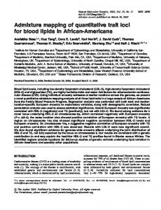
FIG. 1. CPU times for the kernel problems.
Figure 1 shows the total CPU time required for solving the least squares kernel problem in a full genomic scan for two one-QTL and two two-QTL models. The gain in using UQRLS instead of G02DAF is dramatic. The difference is 2–3 orders of magnitude for all problem sizes tested. UQRLS requires 20 and 2 hours 40 minutes respectively for the two-dimensional scans, while G02DAF would need 45 hours and 54 days, respectively. The differences depend both on the reduction of work introduced by the updating procedure and the extra calculations performed by G02DAF. Comparing SQRDC/SQRSL and G02DAF shows that the unnecessarily detailed analysis and robustness of G02DAF are responsible for a 1–2 orders of magnitude increase in computational effort, compared to a routine that computes the QR factorization using the standard algorithm. Hence, a comparison of SQRDC/SQRSL and UQRLS demonstrates the gain of our updating algorithm. Updating reduces the CPU time by approximately one order of magnitude for one-QTL models and slightly less for two-QTL models. Note that this corresponds well to the gain in arithmetic operations derived in Section 6. We now turn to evaluating the convergence properties of the new version of the EM algorithm, presented in Section 8.1. Also in these experiments, we for simplicity refrain from using cofactors, resulting in a standard IM model using ML estimation. The aim of the experiments is to compare the convergence rates of the ECM and EM algorithms. In CIM, xed effects and marker cofactors are mathematically treated in almost exactly the same way, and the results concerning computational demand can equally well be applied to a CIM model. We present results for complete genome scans on the pig data set, calculating the ML estimates and test statistics at 1 cM intervals at 2,259 genomic positions in total. The a priori probabilities of genotypes ®, ¯, and ° were calculated as described by Haley et al. (1994). Again, the purpose of the experiments is to compare the convergence rates of the methods, and the speci c method used to determine the a priori probabilities is not important in this context. There were f D 31 xed effects and g D 2 genetic effects included in the model. We performed the computations using ve versions of the ML solver: ² ECM-null: The ECM algorithm using the null hypothesis parameter estimates as initial values, as is the default of Basten et al. (2001). ² EM-null: The EM algorithm with the null hypothesis estimates as initial values. ² ECM-prev: The ECM algorithm using the parameter estimates from the previous location as initial values.
802
LJUNGBERG ET AL.
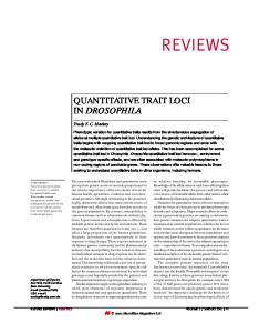
FIG. 2.
Normalized numbers of iterations needed for a full genomic scan.
² EM-prev: The EM algorithm with the previous estimates as initial values. ² EM-LS: The EM algorithm using parameters from the least squares solution as initial values. (The LS solution was obtained using UQRLS, and the work was counted as one EM iteration.) Using ECM-prev and EM-prev, the null hypothesis estimates were used as initial values for the rst position on each chromosome, since there the test statistic function is discontinuous. Figure 2 shows the normalized numbers of iterations for the different ML solver versions. The computational work needed for one iteration is very similar for the two algorithms, the EM algorithm requiring slightly fewer arithmetic operations per iteration than the ECM algorithm. From the results it is clear that the convergence of the EM algorithm is more than twice as fast as the convergence of the ECM version. This is not surprising, since the ECM algorithm is obtained by introducing approximations in the EM algorithm. Also, the results show that much is gained by using the previous parameter estimates as initial values in the next iteration. This was also expected, since the test statistic is mostly a continuous function. There is only need for a restart at discontinuities, i.e., at new chromosomes and when a marker cofactor enters or leaves the model. In this particular experiment, there were no cofactors included, so in a general case there would have to be a restart more often. Then the LS solution should be used rather than the null hypothesis, as the LS solution is inexpensive to obtain if using UQRLS, and is closer to the true ML solution. The experiment above only counts the number of iterations and approximate number of oating number operations needed for them, assuming matrix factorizations are already available. For this problem both iterative methods require only a single factorization, since there are no cofactors included in the model and they all exploit the constant Xf . If marker cofactors are included in the model, the comparison will be even more in favor of our new formulation of the EM algorithm, since we use updating instead of full refactorization of Xf c . The overhead in checking when an update is required is small compared to the gain in computational effort.
10. DISCUSSION Using our new algorithms, the gain in computational ef ciency is enough to make previously intractable QTL analyses realistic, for example permutation testing for multiple QTL scans. A typical permutation test includes 1,000 exhaustive two-dimensional searches.
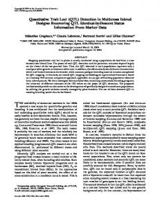
QUANTITATIVE TRAIT LOCI MAPPING Table 1.
803
Approximate CPU Times for Kernel Problem in 1,000 Exhaustive Searches Using the LR Model
Routine
Pig, g D 2
Chicken, g D 2
Pig, g D 8
Chicken, g D 8
G02DAF SQRDC/SQRSL UQRLS
1.2 days 46 min 3.7 min
33 days 5.6 h 40 min
5.2 years 53 days 14 days
148 years 440 days 152 days
In Table 1, the timings for permutation tests are presented. Solving the LR kernel problems corresponding to 1,000 exhaustive searches in two dimensions for the real pig data set would take just under 14 days with UQRLS, 53 days with SQRDC/SQRSL, and 5:2 years with G02DAF. Hence, the amount of time needed to solve the kernel problem makes a full permutation test with exhaustive search in two dimensions impossible if using G02DAF and unattractive with SQRDC/SQRSL. With UQRLS, however, the CPU time needed for the kernel problem is reasonable. Since the 1,000 searches are completely independent, the problem is very easily parallelized by simply assigning each of a number of computers a smaller number of the searches. With a careful implementation of the analysis program and using simple parallelization, it is realistic to routinely perform two-dimensional permutation testing. For example, using a lab with 20 computers, it would be possible to perform the analysis overnight. For accurate detection and location of multiple interacting QTL in large data sets, using IM-based multidimensional search schemes, more elaborate optimization methods will eventually be required. Some work has recently been performed in this area. Carlborg et al. (2000) use a genetic optimization algorithm used for performing a true multidimensional search. Kao and Zeng (1997), Kao et al. (1999), and Zeng et al. (1999) develop the Multiple Interval Mapping (MIM) technique, where the optimization is performed over selected regions in the search space. Also, methods based on sequences of one-dimensional QTL scans have been developed (Jansen and Stam, 1994; Broman, 1997; Jannink and Jansen, 2001), but such schemes may have problems in detecting interacting QTL where the individual QTLs have small independent effects. With a better optimization algorithm than exhaustive search, models with genome scans in three or more dimensions could probably be used without introducing unrealistic computational times, even when combined with permutation testing. Finally, it should be noted that if the kernel routines are replaced by highly ef cient versions, other parts of the QTL analysis program might turn out to be poorly implemented and too time consuming. To construct an ef cient program for accurate multiple QTL scans, other routines might also need optimization efforts.
REFERENCES Andersson, L. 2001. Genetic dissection of phenotypic diversity in farm animals. Nature Rev. Genet. 2, 130–138. Andersson, L., Haley, C., Ellegren, H., Knott, S., Johansson, M., Andersson, K., Andersson-Eklund, L., Edfors-Lilja, I., Fredholm, M., and Hansson, I. 1994. Genetic mapping of quantitative trait loci for growth and fatness in pigs. Science 263, 1771–1774. Basten, C., Weir, B., and Zeng, Z.-B. 2001. QTL Cartographer, Version 1.15. Department of Statistics, North Carolina State University, Raleigh, NC. Björck, Å. 1996. Numerical Methods for Least Squares Problems, Society for Industrial and Applied Mathematics (SIAM), Philadelphia. Broman, K. 1997. Identifying Quantitative Trait Loci in Experimental Crosses. PhD thesis, Deparment of Statistics, University of California, Berkeley. Carlborg, Ö., Andersson, L., and Kinghorn, B. 2000. The use of a genetic algorithm for simultaneous mapping of multiple interacting quantitative trait loci. Genetics 155, 2003–2010. Churchill, G., and Doerge, R. 1994. Empirical threshold values for quantitative trait mapping. Genetics 138, 963–971. Doerge, R. 2002. Mapping and analysis of quantitative trait loci in experimental populations. Nature Rev. Genet., 3, 43–52. Haley, C., and Knott, S. 1992. A simple regression method for mapping quantitative trait loci in line crosses using anking markers. Heredity 69, 315–324.
804
LJUNGBERG ET AL.
Haley, C., Knott, S., and Elsen, J.-M. 1994. Mapping quantitative trait loci in crosses between outbred lines using least squares. Genetics 136, 1195–1207. Jannink, J.-L., and Jansen, R. 2001. Mapping epistatic quantitative trait loci with one-dimensional genome searches. Genetics 157, 445–454. Jansen, R. 1992. A general mixture model for mapping quantitative trait loci by using molecular markers. Theoret. Appl. Genet. 85, 252–260. Jansen, R. 1993. Interval mapping of multiple quantitative trait loci. Genetics 135, 205–211. Jansen, R., and Stam, P. 1994. High resolution of quantitative traits into multiple loci via interval mapping. Genetics 136, 1447–1455. Kao, C.-H., and Zeng, Z.-B. 1997. General formulae for obtaining the MLEs and the asymptotic variance–covariance matrix in mapping quantitative trait loci when using the EM algorithm. Biometrics 53, 653–665. Kao, C.-H., Zeng, Z.-B., and Teasdale, R. 1999. Multiple interval mapping for quantitative trait loci. Genetics 152, 1203–1216. Lander, E., and Botstein, D. 1989. Mapping mendelian factors underlying quantitative traits using RFLP linkage maps. Genetics 121, 185–199. Mackay, T. 2001. Quantitative trait loci in Drosophila. Nature Rev. Genet. 2, 11–21. Martinez, O., and Curnow, R. 1992. Estimating the locations and the sizes of effects of quantitative trait loci using anking markers. Theoret. Appl. Genet. 85, 480–488. Meng, X.-L., and Rubin, D. 1993. Maximum likelihood estimation via the ECM algorithm: A general framework. Biometrika 80, 267–278. O’Leary, D., 1990. Robust regression computation using iteratively reweighted least squares. SIAM J. Matrix Analysis and Applications 11, 466–480. Zeng, Z.-B. 1993. Theoretical basis for separation of multiple linked gene effects in mapping quantitative trait loci. Proc. Natl. Acad. Sci. USA 90, 10972–10976. Zeng, Z.-B. 1994. Precision mapping of quantitative trait loci. Genetics 136, 1457–1468. Zeng, Z.-B., Kao, C.-H., and Basten, C. 1999. Estimating the genetic architecture of quantitative traits. Genet. Res. 74, 279–289.
Address correspondence to: Kajsa Ljungberg Department of Scienti c Computing Uppsala University Box 337 SE-751 05 Uppsala, Sweden E-mail:
[email protected]