Efficient and reliable numerical integration of

JOURNAL OF CHEMICAL PHYSICS

VOLUME 121, NUMBER 2

8 JULY 2004

Efficient and reliable numerical integration of exchange-correlation energies and potentials Andreas M. Ko¨ster,a) Roberto Flores-Moreno, and J. Ulises Reveles Departamento de Quı´mica, CINVESTAV, Avenida Instituto Politećnico Nacional 2508 A.P. 14-740 Me´xico D.F. 07000, Me´xico

共Received 17 February 2004; accepted 15 April 2004兲 An adaptive numerical integrator for the exchange-correlation energy and potential is presented. It uses the diagonal elements of the exchange-correlation potential matrix as a grid generating function. The only input parameter is the requested grid tolerance. In combination with a defined cell function the adaptive grid generation scales almost linear with the number of basis functions in a system. With the adaptive numerical integrator the self-consistent field energy error, which is due to the numerical integration of the exchange-correlation energy, converges with increasing adaptive grid size to a reference value. The performance of the adaptive numerical integration is analyzed using molecules with first, second, and third row elements. Especially for transition metal systems the adaptive numerical integrator shows considerably improved performance and reliability. © 2004 American Institute of Physics. 关DOI: 10.1063/1.1759323兴

available8 –11 and some DFT programs like NRLMOL12 and 13 ALLCHEM rely fully on adaptive numerical integration techniques. In this article, we present an adaptive numerical integrator implemented in the DFT program deMon.14 In the next section the theoretical background for the adaptive numerical integrator is presented. The computational methodology is given in Sec. III. In Sec. IV the accuracy and performance of the adaptive numerical integrator are discussed. Concluding remarks are given in Sec. V.

I. INTRODUCTION

The development of molecular density functional theory 共DFT兲 methods has considerably simplified molecular electronic structure calculations. Using the variational fitting of the Coulomb potential1–3 and the asymptotic expansion of the three-center electron repulsion integrals,4 the numerical evaluation of the exchange-correlation energy and potential matrix becomes the rate-determining step in DFT calculations. On the other hand the accurate numerical integration of the exchange-correlation potential matrix is crucial for the reliability of density functional theory 共DFT兲 methods.5 Therefore, a compromise between efficiency and reliability for the numerical integration has to be found. In most DFT programs fixed grids are used for the numerical integration of the exchange-correlation potential and energy. They are usually adjusted to specific basis sets. Most often these grids are also varying for different chemical elements. For their parametrization the integration of the electronic density and not of the exchange-correlation potential is frequently used. Thus, many test calculations are often necessary to ensure the reliability and efficiency of the numerical integration for a specific problem. In order to avoid numerical instabilities some codes employ large fixed integration grids by default. Of course this can lead to prohibitive expensive calculations for even medium sized systems. A better choice is an adaptive grid that is automatically generated according to a given accuracy. Such a grid can adapt to the basis set, the chemical element, and the exchange-correlation functional. An early approach for the construction of an adaptive grid for DFT methods was outlined by Andzelm and Wimmer.6 A systematic investigation of automatic numerical integration techniques for molecules was given by Pe´rez-Jorda´, Becke, and San-Fabiań.7 Several fast and reliable adaptive grid generation procedures are now

II. ADAPTIVE NUMERICAL INTEGRATOR A. Molecular partition scheme

For the numerical integration the molecular function F(r) is partitioned into atomic contributions as F 共 r兲 ⫽

共1兲

The atomic contributions are defined by normalized atomic weight functions ␻ A (r) F A 共 r兲 ⫽ ␻ A 共 r兲 F 共 r兲

with

兺A ␻ A共 r兲 ⫽1᭙r.

共2兲

With this partitioning scheme a molecular integral I⫽

冕

共3兲

F 共 r兲 dr

can be rewritten as a sum of atomic integrals I⫽

a兲

兺A

冕

F A 共 r兲 dr⫽

兺A I A .

共4兲

The atomic integrals

Electronic mail: [email protected]

0021-9606/2004/121(2)/681/10/$22.00

兺A F A共 r兲 .

681

© 2004 American Institute of Physics

Downloaded 11 Aug 2004 to 169.237.38.255. Redistribution subject to AIP license or copyright, see http://jcp.aip.org/jcp/copyright.jsp

682

Ko¨ster, Flores-Moreno, and Reveles

J. Chem. Phys., Vol. 121, No. 2, 8 July 2004

I A⫽

冕冕冕 ␲

⬁

0

0

2␲

0

F A 共 r A , ␽ A , ␸ A 兲 r A2 sin ␽ A d ␸ A d ␽ A dr A 共5兲

are rearranged into successive one- and two-dimensional integrals I A⫽

冕

⬁

0

I A 共 r A 兲 dr A

共6兲

with

冕冕 ␲

I A共 r A 兲 ⫽

0

2␲

0

F A 共 r A , ␽ A , ␸ A 兲 r A2 sin ␽ A d ␸ A d ␽ A . 共7兲

10

In a precursor of the here described adaptive numerical integrator the normalized atomic weight function was calculated by Becke’s molecular partition scheme15 without atomic size adjustment. For this calculation the confocal elliptic coordinates ␮ AB are defined r A ⫺r B ␮ AB ⫽ . R AB

共8兲

Here r A and r B are distances between a grid point and the atoms A and B, respectively. R AB denotes the internuclear distance. By construction ␮ AB is defined in the interval 关⫺1,1兴. For the calculation of the atomic step function the cubic polynomial 3 1 3 p 共 ␮ AB 兲 ⫽ ␮ AB ⫺ ␮ AB 2 2

共9兲

was suggested. This polynomial posses the following properties: p 共 1 兲 ⫽1,

p 共 ⫺1 兲 ⫽⫺1,

p ⬘ 共 1 兲 ⫽0,

p ⬘ 共 ⫺1 兲 ⫽0.

It has been shown in the literature15 that three iterations of this polynomial f 共 ␮ AB 兲 ⫽p 兵 p 关 p 共 ␮ AB 兲兴其

共10兲

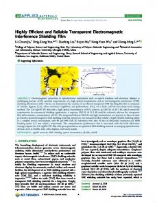
FIG. 1. Comparison of Becke’s cell function 共solid curve兲 with the piecewise defined cell function 共dashed curve兲 described in the text.

The normalized atomic weight function used in the partitioning scheme proposed by Becke has the following form:

␻ 共 r兲 ⫽

P A 共 r兲 . 兺 B P B 共 r兲

共13兲

Thus, the calculation of the atomic weight function involves only atomic coordinates. However, it scales cubic in the number of atoms and can become the rate-determining step in the grid construction. There are several alternative definitions for atomic weight functions 共e.g., Refs. 16 and 17兲 which can be screened and, therefore, show an improved performance. All of them should work fine with an adaptive numerical integrator because it will automatically adapt to the changed weight function. In the adaptive numerical integrator we have implemented a modification of the atomic weight function scheme from Ref. 17 because it resembles most closely the one from Becke. In this approach the cubic polynomial p( ␮ AB ) is substituted by a piecewise defined function as follows: q 共 ␮ AB ;a 兲 ⫽⫺1

᭙ ␮ AB ⭐⫺a,

q 共 ␮ AB ;a 兲 ⫽z 共 ␮ AB ;a 兲 q 共 ␮ AB ;a 兲 ⫽1

᭙⫺a⬍ ␮ AB ⬍a,

᭙ ␮ AB ⭓a.

result in a numerical stable partitioning. This approach was also adopted in the precursor of the adaptive numerical integrator and the normalized cell function between two atoms A and B, defined in the interval 关0,1兴 is calculated as

The polynomial z( ␮ AB ;a) is a scaled p( ␮ AB ) polynomial

1 s 共 ␮ AB 兲 ⫽ 关 1⫺ f 共 ␮ AB 兲兴 2

satisfying the following conditions:

⫽

1 3 ⫺3 ␮ AB ⫺4 兲 2 兴关共 ␮ AB ⫺1 兲 8 共 ␮ AB ⫹2 兲 4 共 ␮ AB 16 384 9 7 5 3 ⫻ 关 ␮ AB ⫺9 ␮ AB ⫹27␮ AB ⫺39␮ AB ⫹36␮ AB ⫹32兴 .

共11兲 This cell function represents a smoothed out step function. The atomic weight function is then defined over these cell functions by P A 共 r兲 ⫽

兿

B⫽A

s 共 ␮ AB 兲 .

共12兲

z 共 ␮ AB ;a 兲 ⫽

冉冊冉冊

3 ␮ AB 1 ␮ AB ⫺ 2 a 2 a

3

z 共 ␮ AB ⫽a 兲 ⫽1,

z 共 ␮ AB ⫽⫺a 兲 ⫽⫺1,

z ⬘ 共 ␮ AB ⫽a 兲 ⫽0,

z ⬘ 共 ␮ AB ⫽⫺a 兲 ⫽0.

共14兲

Different to Ref. 17 we iterate q( ␮ AB ;a), analog to p( ␮ AB ), three times in order to obtain the cell function. This ensures that the cell function s 共 ␮ AB ;a 兲 ⫽ 21 共 1⫺ p 兵 p 关 q 共 ␮ AB ;a 兲兴其兲

共15兲

is for a⫽1 identical with the cell function of Becke’s partitioning scheme. The same holds for the normalized atomic weight functions. In our implementation a cutoff parameter of a⫽0.7 is used. In Fig. 1 the two cell functions are compared. As can be seen from this figure, the cell function is



Integration of exchange-correlation energies

683

Also the Euler-Maclaurin quadrature can be used for the radial numerical integration in deMon. For the transformation of the abscissas from the interval 关⫺1,1兴 to the interval 关0,⬁兴 the following parameter-free transformation formula is used: r A⫽

FIG. 2. Computational time for the adaptive grid construction for a series of alkenes (C48H98 , C72H146 , C96H194 , C120H242 , C144H290 , C168H338 and C192H386) on a SGI R14000 共500 MHz兲 node. The dashed line refers to the grid construction with the cell function from Becke 共11兲, whereas the solid line refers to the grid construction with the screened cell function 共15兲.

冉冊

2 1 ln ⇔x A ⫽1⫺2 共 1⫺r A 兲 . ln 2 1⫺x A

共19兲

It has been shown in the literature24,25 that this transformation formula can also be used for fixed grids. As in most other implementations two-dimensional Gauss-type quadrature schemes 共Gauss–Markov兲 for the unit sphere defined by Lebedev26 –30 are used for the angular integration in the adaptive numerical integrator. This quadrature schemes exactly integrate real spherical harmonics S lm ( ␽ , ␸ ) with 兩 m 兩 ⭐l up to a maximum degree L (0⭐l ⭐L) that is used to characterize the corresponding angular grid. In the adaptive numerical integrator angular grids with 6 共3兲, 14 共5兲, 26 共7兲, 38 共9兲, 50 共11兲, 86 共15兲, 110 共17兲, 146 共19兲, 194 共23兲, 302 共29兲, 434 共35兲, 590 共41兲, 770 共47兲, 974 共53兲 and 1202 共59兲 points are available. The numbers in brackets are the characteristic L values of the angular grids. The abscissas and weights of these grids have been recalculated and are stored with 20 significant digits.31

C. Adaptive grid generation

more step functionlike. Because of the form of the cell function an efficient screening of the normalized atomic weight function can be achieved.17 In Fig. 2 the computational timings on a SGI R14000 共500 MHz兲 node for the adaptive grid construction of a series of alkenes are depicted. The DZVP basis and A2 auxiliary function set18 were used. The dashed curve shows the timing for the grid construction using the cell function from Becke 共11兲, whereas the solid curve shows the same timing using the screened cell function 共15兲. The performance improvement is large as Fig. 2 shows. Moreover, with the screened cell function the adaptive grid generation scales almost linear with the number of basis functions. B. Quadrature schemes

For the radial numerical integration of I A in Eq. 共6兲

冕

b

a

n

I A 共 x 兲 dx⬇

兺 w iI A共 x i 兲

共16兲

i⫽1

many quadrature schemes have been suggested.19–23 In the adaptive numerical integrator the transformed Gauss– Chebyshev quadrature of the second kind is used. The corresponding abscissas x i and weights ␻ i are defined by7 x i⫽

冋

冉冊册

n⫹1⫺2i 2 2 i␲ 1⫹ sin2 ⫹ n⫹1 ␲ 3 n⫹1 ⫻cos

w i⫽

冉冊冉冊冉冊

i␲ i␲ sin , n⫹1 n⫹1

16 i␲ sin4 . 3 共 n⫹1 兲 n⫹1

共17兲共18兲

As described in Ref. 10 the adaptive adjustment of the radial numerical integration causes instabilities in the adaptive grid generation procedure. Moreover, there is no need for such an adjustment if adaptive angular grids are employed. Therefore, the order of the radial quadrature is determined by the following empirical formula: n Ar ⫽max关 20,⫺5 共 3 log ⑀ Grid⫺t A ⫹6 兲兴 .

共20兲

Here ⑀ Grid is the requested tolerance for the numerical integration and t A the row of atom A in the periodic table. This formula ensures that enough radial quadrature points are supplied for the angular adaptive grid generation procedure. This procedure will then take care that radial points defining rather unimportant shells are represented by angular grids of small size. For instance small angular grids will be selected for radial points close to the corresponding nucleus where the electronic charge distribution is spherical. This fact also justifies the common pruning of fixed grids.32 After the definition of the radial quadrature points angular grids have to be selected for each radial shell. For this adaptive grid generation a generating function is necessary. To be reliable, this function has to contain all information about the molecular system. Moreover, the grid generating function must include information about the atomic orbital matrix elements, because the final grid is used in the selfconsistent field 共SCF兲 procedure for the numerical integration of the exchange-correlation potential matrix. In the precursor of the here described adaptive numerical integrator10 the diagonal elements of the overlap matrix S ␮␮ were used as a grid generating function. Because the convergence of the numerical integration is directly related to the absolute value of the corresponding quantity this approach ensured the con-


684



step with the screened cell function is negligible in the computational time 共see Fig. 2兲 this procedure is very efficient. III. COMPUTATIONAL METHOD

All calculations were performed with deMon14 using the variational approximation of the Coulomb potential proposed by Dunlap, Connolly, and Sabin.1 The approximated density was expanded in atomic centered primitive Hermite Gaussian functions.4 For the fitting, the auxiliary function set A218 was used. The structures of all molecules were optimized using the DZVP basis18 and the local exchange-correlation functional proposed by Vosko, Wilk, and Nusair.34 The reported test calculations were performed with the gradient corrected exchange functional from Becke35 and the correlation functional from Lee, Yang, and Parr.36,37 In all cases the adaptive grid was build without exploiting the molecular symmetry. IV. DISCUSSION

FIG. 3. Flowchart for the adaptive grid generation with the diagonal elements of the exchange-correlation matrix V ␮␮ as generating function.

vergence of the full overlap matrix and, therefore, the convergence of the numerical integration of the electron density. From the experiences of this approach we have learned that the reliable numerical integration of the electron density is not sufficient to ensure the reliable numerical integration of the exchange-correlation potential. Therefore, the S ␮␮ elements are substituted by the corresponding diagonal elements of the exchange-correlation potential matrix V ␮␮ in the grid generating function of the adaptive numerical integrator. The flowchart for the adaptive grid generation is depicted in Fig. 3. For each atom the number of radial shells is calculated using Eq. 共20兲. In a next step the limits for the angular quadrature are set. In our implementation an upper L max value (L max⫽5–6 log ⑀Grid) is used in order to avoid a waste of grid points for some radial shells in the bonding region. This limit was chosen carefully in order to ensure the reliability of the grid. It improves the grid efficiency significantly for grid tolerances in the range of 10⫺4 to 10⫺8 . After the radial shells and angular quadrature limits are defined the algorithm loops over all shells at the processed atom A. For each radial shell a Lebedev grid size is then iteratively determined based on the integration error shown in Fig. 3. Finally, grid points with negligible weights ( ␻ (r)⭐10⫺8 ⑀ Grid) are screened. For the calculation of the diagonal elements of the exchange-correlation potential matrix V ␮␮ an electronic density is necessary. By default, the converged SCF density is used in deMon. Therefore, the adaptive grid is generated twice, first with the start density and second with the converged SCF density. With this grid the SCF is then converged again. This procedure guarantees an optimal adaption of the grid. It has been shown that these grids are also well suited for geometry optimizations.33 Because the grid generation

In Tables I and II the results of the adaptive grid generation for molecules with first row elements are presented. Table I reports the results using Becke’s cell function 共11兲 and Table II reports the results using the screened cell function defined by Eq. 共15兲. For each molecule the number of generated grid points 共first row兲 and the accuracy of the converged self-consistent field 共SCF兲 energy 共second row兲 are listed. The energy accuracy in the tables is given in ␮Hartree and is calculated with respect to a fixed grid using 200 radial shells each carrying a Lebedev grid with 1202 points (L ⫽59). The number of grid points and the total energy 共in hartree兲 obtained with this reference grid are given in the last columns of the tables. For the reference grid Becke’s cell function was used. As can be seen from Tables I and II, the energy of all systems converges with increasing adaptive grid size 共decreasing grid tolerance兲 to the reference energy. This behavior is independent from the used cell function. With the smallest adaptive grid reported 共grid tolerance 10⫺4 ), that corresponds to the COARSE grid option in deMon, a energy accuracy better than 200 ␮Hartree is reached for both cell functions used. In order to obtain this accuracy roughly 2000 to 3000 grid points per atom are generated. With a grid tolerance of 10⫺5 共MEDIUM grid option, this is the default in deMon兲 the energy error for the molecules containing first row elements only is reduced to less than 20 ␮Hartree. This grid accuracy is sufficient for frequency analysis or other higher derivative calculations. It roughly doubles the number of grid points per atom of the previous COARSE grid. A 10⫺6 grid tolerance 共FINE grid option兲 reduces the energy error for the molecules in Tables I and II to a few ␮Hartree. This grid can already be used as a reference grid. The comparison of Tables I and II shows that the adaptive grid performance with the screened cell function is very similar to the one with the cell function from Becke. In order to demonstrate the stability of the adaptive generated grid the orientation dependency of the SCF energy of benzene is depicted in Fig. 4. For the sampling the benzene molecule was rotated by increments of 30° around the angles




685

TABLE I. The total number of grid points 共first row兲 and the deviation of the SCF energy from the reference energy 共last column兲 in ␮Hartree 共second row兲 for first row molecules using different adaptive grid tolerances. For the numerical integration the cell function of Becke 共11兲 was employed. Requested tolerance Molecule LiH LiF BF3 CO C5 H12 C6 H6 NO N2 H2 O O2 HF F2

10⫺4

10⫺5

10⫺6

10⫺8

10⫺10

Reference 共200,1202兲

4010 31 3132 5 7016 16 3053 19 25 500 45 22 277 37 3067 75 3240 1 4055 56 2892 5 2577 9 3450 21

9519 3 7803 2 16 701 3 6068 3 57 176 9 53 323 1 5815 7 5574 19 8422 4 5894 1 4781 3 6838 6

18 416 1 15 463 0 33 893 0 12 209 0 122 111 2 102 788 1 11 143 2 11 262 0 16 839 1 11 578 1 8809 0 13 018 1

50 954 0 44 059 0 103 463 0 31 983 0 378 700 0 302 077 0 32 090 0 31 094 0 47 095 0 33 816 0 23 937 0 34 726 0

95 072 0 86 334 0 206 684 0 62 718 0 766 336 0 608 257 0 69 232 0 60 914 0 108 243 0 78 388 0 51 512 0 73 520 0

383 045 ⫺8.071 420 385 472 ⫺107.442 024 769 154 ⫺324.605 622 383 077 ⫺113.316 230 3 117 212 ⫺197.679 859 2 230 970 ⫺232.185 753 383 115 ⫺129.902 532 381 910 ⫺109.525 418 573 343 ⫺76.432 522 384 356 ⫺150.351 619 384 297 ⫺100.460 389 386 810 ⫺199.560 852

TABLE II. The total number of grid points 共first row兲 and the deviation of the SCF energy from the reference energy 共last column兲 in ␮Hartree 共second row兲 for first row molecules using different adaptive grid tolerances. For the numerical integration the screened cell function of Eq. 共15兲 was employed. Requested tolerance Molecule LiH LiF BF3 CO C5 H12 C6 H6 NO N2 H2 O O2 HF F2

10⫺4

10⫺5

10⫺6

10⫺8

10⫺10


3847 3 4186 5 8353 31 3472 6 26 803 199 27 740 21 3050 15 3268 37 4667 91 3064 13 2640 3 2944 32

9486 2 9551 5 18 433 3 6401 2 62 158 11 57 590 4 6374 4 6258 2 11 013 2 6764 4 5344 0 6518 1

18 464 0 18 467 0 32 859 1 11 411 0 120 154 4 105 905 1 11 045 0 11 062 1 21 396 0 11 318 0 9700 0 12 818 0

48 625 0 46 758 0 94 544 0 30 253 0 328 697 1 281 546 0 29 783 0 28 875 0 56 576 0 30 878 0 25 717 0 34 118 0

93 583 0 93 321 0 197 051 0 72 926 0 687 336 0 550 139 0 70 701 0 71 050 0 122 976 0 73 856 0 64 463 0 76 056 0

383 045 ⫺8.071 420 385 472 ⫺107.442 024 769 154 ⫺324.605 622 383 077 ⫺113.316 230 3 117 212 ⫺197.679 859 2 230 970 ⫺232.185 753 383 115 ⫺129.902 532 381 910 ⫺109.525 418 573 343 ⫺76.432 522 384 356 ⫺150.351 619 384 297 ⫺100.460 389 386 810 ⫺199.560 852


686



FIG. 4. Orientation dependency of the SCF energy 共b兲 and grid point number 共c兲 of benzene. The rotation angles ␣ and ␤ are defined in 共a兲. The absolute energy deviations are reported with respect to the unpruned 共200,1202兲 reference grid energy given in Table I. The changes in grid points are reported with respect to the ␣⫽0° and ␤⫽0° orientation. The left entries 共b兲 and 共c兲 are for the MEDIUM and the right for the FINE adaptive grid.

␣ and ␤ 关see Fig. 4共a兲 for the angle definition兴 in the range from 0° to 180°. The screened cell function defined by Eq. 共15兲 was used. For the MEDIUM adaptive grid 关left in Figs. 4共b兲 and 4共c兲兴 a mean absolute energy deviation of 8 ␮Hartree from the reference grid is observed. The maximum energy deviation is 28 ␮Hartree. For the FINE adaptive grid 关right in Figs. 4共b兲 and 4共c兲兴 the corresponding mean and maximum energy deviations are 3 and 7 ␮Hartree, respectively. This indicates that the adaptive grid stabilities are in the same energy range as the reported grid accuracies in

Tables I and II. As can be seen from Fig. 4共c兲 the adaptive grids respond to the different orientations by changing the number of grid points. For the benzene molecule the average deviation of grid points is in the range of 3000 points. In Tables III and IV the corresponding data for molecules with second row elements are listed. Also for these systems the energy converges with increasing adaptive grid size to the reference energy, independent from the used cell function. A grid tolerance of 10⫺4 usually results in energy errors less than 300 ␮Hartree. However, the P4 O6 calculation




687

TABLE III. The total number of grid points 共first row兲 and the deviation of the SCF energy from the reference energy 共last column兲 in ␮Hartree 共second row兲 for second row molecules using different adaptive grid tolerances. For the numerical integration the cell function of Becke 共11兲 was employed. Requested tolerance Molecule BCl3 NCl3 Mg共C5 H5 ) 2 AlCl3 Si2 OH6 P4 O6 H2 S SF6 S2 HCl ClF5

10⫺4

10⫺5

10⫺6

10⫺8

10⫺10


7787 105 8611 69 43 799 84 7968 65 13 809 282 22 660 354 4754 3 12 524 94 3606 118 2850 222 11 040 103

17 134 8 19 352 4 99 774 6 17 750 11 36 664 5 46 144 23 10 468 9 28 964 3 7706 5 6175 8 26 598 1

34 116 0 38 278 0 185 957 3 38 240 1 75 725 2 91 851 2 20 815 1 51 784 1 14 688 0 11 278 0 48 749 1

104 727 0 108 011 0 525 913 1 111 003 0 233 500 0 257 963 0 57 943 0 154 374 1 40 912 0 28 816 0 135 727 1

195 231 0 204 297 0 1 039 357 0 218 824 0 476 162 0 492 784 0 122 124 0 293 902 1 87 200 0 60 609 0 262 549 1

747 166 ⫺1405.417 617 748 298 ⫺977.651 583 3 822 080 ⫺587.029 389 743 050 ⫺1623.082 236 1 685 498 ⫺657.812 376 1 847 596 ⫺1816.872 041 567 577 ⫺399.349 820 1 335 241 ⫺997.192 650 372 387 ⫺796.290 656 377 115 ⫺460.756 809 1 147 703 ⫺959.099 590

with the cell function of Becke shows an energy error of 354 ␮Hartree. This indicates that the COARSE grid is no longer sufficient to obtain reliable energies. The energy accuracy improves considerably for a grid tolerance of 10⫺5 . Similar to the first row molecules this grid tolerance gives also for the second row molecules an energy accuracy in the range of

20 ␮Hartree. Thus, the MEDIUM grid with a grid tolerance of 10⫺5 is also for molecules containing second row elements sufficient. On average, this grid produces 4000 to 5000 points per atom. A more economic grid for molecules containing second row atoms can be obtained by choosing a grid tolerance between 10⫺4 and 10⫺5 . With a grid tolerance

TABLE IV. The total number of grid points 共first row兲 and the deviation of the SCF energy from the reference energy 共last column兲 in ␮Hartree 共second row兲 for second row molecules using different adaptive grid tolerances. For the numerical integration the screened cell function of Eq. 共15兲 was employed. Requested tolerance Molecule BCl3 NCl3 Mg共C5 H5 ) 2 AlCl3 Si2 OH6 P4 O6 H2 S SF6 S2 HCl ClF5

10⫺4

10⫺5

10⫺6

10⫺8

10⫺10


7659 132 6930 87 46 071 108 7883 191 16 279 45 20 565 285 5094 113 11 392 41 3500 113 2828 63 10 202 172

18 325 2 16 200 1 98 382 1 19 264 3 37 046 1 45 526 22 11 824 2 25 918 5 6926 1 5948 0 23 124 8

33 457 1 32 240 0 174 133 1 37 437 1 76 539 0 82 678 1 22 672 0 49 386 0 13 290 1 10 731 1 45 523 1

96 127 0 97 075 0 461 314 1 113 148 0 224 309 0 234 860 1 65 127 0 139 074 1 36 786 0 30 773 0 127 092 1

181 762 0 185 786 0 925 529 0 214 703 0 435 674 0 441 434 1 134 485 0 266 196 1 84 440 0 69 749 0 237 437 1

747 166 ⫺1405.417 617 748 298 ⫺977.651 583 3 822 080 ⫺587.029 389 743 050 ⫺1623.082 236 1 685 498 ⫺657.812 376 1 847 596 ⫺1816.872 041 567 577 ⫺399.349 820 1 335 241 ⫺997.192 650 372 387 ⫺796.290 656 377 115 ⫺460.756 809 1 147 703 ⫺959.099 590


688



TABLE V. The total number of grid points 共first row兲 and the deviation of the SCF energy from the reference energy 共last column兲 in ␮Hartree 共second row兲 for transition metal and weakly bonded systems using different adaptive grid tolerances. For the numerical integration the cell function of Becke 共11兲 was employed. Requested tolerance Molecule V2 TiCl4 CrF6 Mn2 (CO) 10 FeC6 H4 O4 Ni共CO) 4 Cu8 MoF6 NH3 BF3 PH3 BH3 (H2 O) 2

10⫺4

10⫺5

10⫺6

10⫺8

10⫺10


4832 24 9797 323 14 812 32 41 280 81 26 987 57 16 870 135 19 887 1266 14 608 28 12 744 80 11 614 87 7954 1

9968 4 24 239 12 30 980 2 98 413 30 66 867 6 36 306 9 40 618 29 32 498 50 32 107 5 26 965 10 16 211 12

17 630 1 48 906 4 62 132 0 200 011 1 137 598 1 71 765 2 78 468 8 64 784 5 63 246 1 54 275 0 36 277 1

45 524 0 145 281 0 185 332 1 599 598 0 401 730 0 219 944 0 200 861 1 178 806 0 201 417 0 183 206 0 117 606 0

96 007 0 265 656 0 345 207 1 1 132 815 0 805 600 1 450 672 0 374 202 0 345 854 0 398 523 0 394 379 0 290 257 0

362 551 ⫺1887.705 649 924 055 ⫺2690.264 185 1 331 625 ⫺1643.605 982 4 034 822 ⫺3435.394 897 2 769 917 ⫺1795.608 964 1 691 963 ⫺1961.592 133 1 417 248 ⫺13 122.526 474 1 331 961 ⫺4576.556 960 1 511 651 ⫺381.1903 66 1 499 867 ⫺369.724 641 1 139 489 ⫺152.872 366

of 10⫺6 the energy error for molecules containing second row elements is reduced to a few ␮Hartree, too. Again the comparison of Tables III and IV shows the very similar performance of the adaptive grid with the two different cell functions. In Tables V and VI the results of the adaptive grid gen-

eration for transition metal and weakly bonded systems are listed. The tables are organized like Tables I and II. For these systems the energy converges with increasing grid size to the reference energy, too. As can be seen from Tables V and VI the COARSE grid with a grid tolerance of 10⫺4 can introduce large energy errors as in the case of the Cu8

TABLE VI. The total number of grid points 共first row兲 and the deviation of the SCF energy from the reference energy 共last column兲 in ␮Hartree 共second row兲 for transition metal and weakly bonded systems using different adaptive grid tolerances. For the numerical integration the screened cell function of Eq. 共15兲 was employed. Requested tolerance Molecule V2 TiCl4 CrF6 Mn2 (CO) 10 FeC6 H4 O4 Ni共CO) 4 Cu8 MoF6 NH3 BF3 PH3 BH3 (H2 O) 2

10⫺4

10⫺5

10⫺6

10⫺8

10⫺10


4186 307 9572 239 12 260 128 42 714 202 31 305 82 18 381 73 16 575 1350 12 448 88 14 696 37 14 347 99 9065 32

9364 4 23 379 15 28 146 7 97 095 3 68 944 6 39 691 7 40 626 35 28 720 2 33 574 1 33 310 5 19 636 5

16 242 1 44 499 1 57 412 1 187 378 2 129 765 6 69 235 1 71 519 12 57 024 3 65 071 0 63 591 1 40 425 1

44 136 0 134 530 0 168 296 1 511 572 0 360 329 1 192 510 0 188 203 1 168 158 0 180 001 0 181 187 0 118 439 0

105 698 0 265 189 0 310 425 1 1 011 548 0 714 102 1 429 175 0 354 824 1 318 536 0 358 928 0 369 036 0 267 996 0

362 551 ⫺1887.705 649 924 055 ⫺2690.264 185 1 331 625 ⫺1643.605 982 4 034 822 ⫺3435.394 897 2 769 917 ⫺1795.608 964 1 691 963 ⫺1961.592 133 1 417 248 ⫺13 122.526 474 1 331 961 ⫺4576.556 960 1 511 651 ⫺381.190 366 1 499 867 ⫺369.724 641 1 139 489 ⫺152.872 366




689

TABLE VII. Comparison of adaptive grids with two pruned fixed grids. The first row lists the total number of grid points and the second row the deviation of the SCF energy from the reference energy 共last column兲 in ␮Hartree. For the numerical integration the cell function of Becke 共11兲 was employed. Requested tolerance Molecule V2 TiCl4 CrF6 Mn2 (CO) 10 FeC6 H4 O4 Ni共CO) 4 Cu8 MoF6

10⫺4

10⫺5

10⫺6

(50,194)p

(75,302)p

4832 24 9797 323 14 812 32 41 280 81 26 987 57 16 870 135 19 887 1266 14 608 28

9968 4 24 239 12 30 980 2 98 413 30 66 867 6 36 306 9 40 618 29 32 498 50

17 630 1 48 906 4 62 132 0 200 011 1 137 598 1 71 765 2 78 468 8 64 784 5

8482 1789 14 693 677 21 060 862 61 874 1970 41 298 1264 26 503 1474 32 575 14 503 23 700 4297

21 188 1 39 248 63 55 570 151 162 093 64 109 439 12 69 063 12 82 250 387 61 544 264

cluster. Therefore, this grid tolerance should not be used for transition metal containing systems. With a grid tolerance of 10⫺5 reliable energies for these systems are obtained. This grid produces 4000 to 5000 points per atom. Again the energy error is reduced to a few ␮Hartree if a grid tolerance of 10⫺6 is used. The difference between the two cell functions is most notable for V2 with a grid tolerance of 10⫺4 . For the more reliable grid tolerances the difference is again small. The adaptive grids of the weakly bonded systems NH3 BF3 , PH3 BH3 and the water dimer show a similar behavior as for molecules containing first and second row elements. This indicates that the performance of the adaptive grid is independent from the bonding situation in the system. In fact this is not too surprising because the adaptive grid incorporates information about the basis set and the exchange-correlation functional. If these quantities are well suited for the description of the interaction the adaptive numerical integrator will produce a grid suitable for the reliable numerical integration. The size of the basis set strongly influences the number of the grid points produced by the adaptive numerical integrator. Large diffuse basis sets, like the ones used for polarizability calculations, need considerably more grid points per atom as the DZVP basis set used here. A factor of two is not uncommon. The effect of the exchange-correlation functional is much less pronounced. In general gradient corrected functionals need more grid points 共roughly 10%兲 than local functionals. The adaptive numerical integrator described in this article takes automatical care to these effects. Table VII compares the performance of the adaptive grids with two pruned fixed grids. For some transition metals the adaptive grids generated by grid tolerances of 10⫺4 , 10⫺5 , and 10⫺6 are compared with the (50,194)p and (75,302)p fixed grids. As a reference, the 共200,1202兲 fixed grid reported in Tables V and VI is used again. In the fixed grid notation the first entry refers to the number of radial shells and the second to the number of angular grid points of

the Lebedev grid located on each of these radial shells. The letter p indicates a pruned grid. As in the previous tables the number of grid points 共first row兲 and the energy accuracy 共second row兲 in ␮Hartree are reported in Table VII. For all calculations the cell function of Becke has been used. Table VII shows that the small pruned fixed grid (50,194)p produces huge errors in the exchange-correlation energy of the studied transition metal systems. With the larger pruned fixed grid (75,302)p these errors are diminished. However, even with the (75,302)p grid energy errors larger than 300 ␮Hartree may be observed as the Cu8 cluster demonstrates. This error is large enough to influence sensitive quantities like frequencies or other higher derivatives. Therefore, we cannot recommend this grid for the reliable integration of the exchange-correlation energy of transition metal systems. The improved performance of the adaptive grids is easily seen from Table VII. In particular, the adaptive grid with a grid tolerance of 10⫺5 shows a considerably improved energy accuracy with much less points as the fixed (75,302)p grid. This underlines the advantage of adaptive grid generation techniques in general. In order to gain more insight into the performance difference of the fixed and adaptive grids the distribution of the radial grid points and the sizes of the angular grids are depicted for the vanadium atom in V2 共a兲 and the molybdenum atom in MoF6 共b兲 in Fig. 5. The connection lines are only to guide the eye. The MEDIUM adaptive 共grid tolerance 10⫺5 ) and COARSE fixed grids are compared because for these two grids the number of grid points is similar but the accuracy is very different 共see Table VII兲. As Fig. 5 shows the adaptive grid concentrates the grid points in a much smaller radial region as the fixed grid. The use of a few very large angular grid is obviously important for the overall grid accuracy. The comparison of Figs. 5共a兲 and 5共b兲 shows a strong system dependency of the adaptive grid point distribution. In V2 关Fig. 5共a兲兴 a large broadening of the adaptive grid point distribution can be observed.


690



The grid efficiency can be tuned by the requested grid tolerance. It is possible to generate reliable grids with less than 3000 points per atom. The convergence of the energy error with respect to the adaptive grid size allows successive improvements of the numerical integration during a computational project. This combines efficiency with reliability.

ACKNOWLEDGMENT

This work was financially supported by the CONACYT Project Nos. G34037-E and 40379-F. R.F.M. and J.U.R. greatfully acknowledge CONACyT Ph.D. fellowships 共Nos. 163442 and 154871兲. 1

FIG. 5. Angular grid sizes of the vanadium atom in V2 共top兲 and the molybdenum atom in MoF6 共bottom兲. The pruned fixed grid (50,194)p 共䊉兲 is compared with an adaptive grid generated with a numerical tolerance of 10⫺5 共⫹兲. The connection lines are only to guide the eye.

V. CONCLUSION

With the adaptive numerical integrator presented in this article an efficient and reliable numerical integration of the exchange-correlation energy and potential is possible. Due to the introduction of a screened cell function the grid generation step is computationally cheap and scales almost linearly with the basis set size. Even so this step has to be performed twice an efficient adaptive grid generation is obtained. Because the adaptive grid adjusts automatically to the molecular structure, the basis set, and the exchange-correlation potential, an increased reliability of the numerical integration is achieved. The default adaptive grid in deMon with a grid tolerance of 10⫺5 performs well for molecules containing first, second, and third row elements, including weakly bonded systems. Recent results from one of the authors 共R.F.M.兲 suggest that this grid is also well suited for heavier elements using effective core potentials. With this grid, 4000 to 5000 points per atom are generated for a double-zeta valence polarization basis set. This number can increase up to a factor of two if a more extended basis set is used. This is important in order to ensure the reliability of the grid independent form the used basis set. The energy error of this grid is less than 100 ␮Hartree. There- fore, this grid can be used for energy and derivative calculations.

B. I. Dunlap, J. W. D. Connolly, and J. R. Sabin, J. Chem. Phys. 71, 4993 共1979兲; J. W. Mintmire and B. I. Dunlap, Phys. Rev. A 25, 88 共1982兲. 2 O. Vahtras, J. Almlo¨f, and M. W. Feyereisen, Chem. Phys. Lett. 213, 514 共1993兲. 3 B. I. Dunlap, J. Mol. Struct.: THEOCHEM 529, 37 共2000兲. 4 A. M. Ko¨ster, J. Chem. Phys. 118, 9943 共2003兲. 5 J. M. L. Martin, C. W. Bauschlicher, Jr., and A. Ricca, Comput. Phys. Commun. 133, 189 共2001兲. 6 J. Andzelm and E. Wimmer, J. Chem. Phys. 96, 1280 共1991兲. 7 J. M. Pe´rez-Jorda´, A. Becke, and E. San-Fabiań, J. Chem. Phys. 100, 6520 共1994兲. 8 M. R. Pederson and K. A. Jackson, Phys. Rev. B 41, 7453 共1990兲. 9 B. Delley, in Modern Density Functional Theory: A Tool for Chemistry, edited by P. Politzer and J. M. Seminario 共Elsevier, New York, 1994兲. 10 M. Krack and A. M. Ko¨ster, J. Chem. Phys. 108, 3226 共1998兲. 11 M. Challacombe, J. Chem. Phys. 113, 10 037 共2000兲. 12 M. R. Pederson, D. V. Porezag, J. Kortus, K. A. Jackson, and D. C. Patton, NRLMOL, USN, Research Laboratory, Washington, D.C. 20375. 13 A. M. Ko¨ster, M. Krack, M. Leboeuf, and B. Zimmermann, ALLCHEM, Universita¨t Hannover, Hannover, Germany, 1998. 14 A. M. Ko¨ster, R. Flores-Moreno, G. Geudtner, A. Goursot, T. Heine, J. U. Reveles, A. Vela, and D. R. Salahub, deMon, NRC, Canada, 2003. 15 A. D. Becke, J. Chem. Phys. 88, 2547 共1987兲. 16 J. Baker, J. Andzelm, A. Scheiner, and B. Delley, J. Chem. Phys. 101, 8894 共1994兲. 17 R. E. Stratmann, G. E. Scuseria, and M. J. Frisch, Chem. Phys. Lett. 257, 213 共1996兲. 18 N. Godbout, D. R. Salahub, J. Andzelm, and E. Wimmer, Can. J. Phys. 70, 560 共1992兲. 19 C. W. Murray, N. C. Handy, and G. J. Laming, Mol. Phys. 78, 997 共1993兲. 20 O. Treutler and R. Ahlrichs, J. Chem. Phys. 102, 346 共1994兲. 21 M. E. Mura and P. J. Knowles, J. Chem. Phys. 104, 9848 共1996兲. 22 ˚ . Malmqvist, and L. Gagliardi, Theor. Chem. Acc. 106, 178 R. Lindh, P.-A 共2001兲. 23 P. M. W. Gill and S.-H. Chien, J. Comput. Chem. 24, 732 共2003兲. 24 G. Hong, M. Dolg, and L. Li, Int. J. Quantum Chem. 80, 201 共2000兲. 25 G. Hong, M. Dolg, and L. Li, Chem. Phys. Lett. 334, 396 共2001兲. 26 V. I. Lebedev, Zh. Vychisl. Mat. Mat. Fiz. 15, 48 共1975兲. 27 V. I. Lebedev, Zh. Vychisl. Mat. Mat. Fiz. 16, 293 共1976兲. 28 V. I. Lebedev, Sibirsk. Mat. Zh. 18, 132 共1977兲. 29 V. I. Lebedev and A. L. Skorokhodov, Rus. Acad. Sci. Dokl. Math. 45, 587 共1992兲. 30 V. I. Lebedev, Rus. Acad. Sci. Dokl. Math. 50, 283 共1995兲. 31 A. M. Ko¨ster, Habilitation Thesis, Universita¨t Hannover, Hannover, Germany, 1998. 32 P. M. W. Gill, B. G. Johnson, and J. A. Pople, Chem. Phys. Lett. 209, 506 共1993兲. 33 J. U. Reveles and A. M. Ko¨ster, J. Comput. Chem. 25, 1109 共2004兲. 34 S. H. Vosko, L. Wilk, and M. Nusair, Can. J. Phys. 58, 1200 共1980兲. 35 A. D. Becke, Phys. Rev. A 38, 3098 共1988兲. 36 C. Lee, W. Yang, and R. G. Parr, Phys. Rev. B 37, 785 共1988兲. 37 B. Miehlich, A. Savin, H. Stoll, and H. Preuss, Chem. Phys. Lett. 157, 200 共1989兲.


Efficient and reliable numerical integration of

Efficient and reliable numerical integration of

Suggest Documents

RELIABLE INTEGRATION OF CONTINUOUS

Numerical Integration and Differentiation

Highly Efficient and Reliable Transparent

Numerical Integration

Efficient Numerical Integration of Dynamical Systems based on

NUMERICAL INTEGRATION OF CONSTRAINED

EFFICIENT NUMERICAL CONTINUATION AND STABILITY ...

GEOMETRIC NUMERICAL INTEGRATION OF NONHOLONOMIC

Numerical Methods of Integration

Performance Analysis of Numerical Integration

Efficient and Reliable Broadcast in Intervehicle Communication ...

A Reliable and Energy-Efficient Classifier

Efficient, continuous and reliable Data Management

i Efficient and Reliable Mathematical Modeling

Efficient and Reliable Template Set Matching for

A Reliable and Distributed LIMS for Efficient

facilitating efficient and reliable monitoring through hamsa

Toward Cost-Efficient and Reliable Unit ... - ee.washington.edu

ZipWeave: Towards Efficient and Reliable ... - WordPress.com

Highly Efficient and Reliable Transparent ... - ACS Publications

Numerical Integration or Quadrature

Efficient Gluing of Numerical Continuation and a

Efficient Gluing of Numerical Continuation and a

Rapid and Efficient Conversion of Integration-Free