Jul 8, 1999 - by Wall and Neuhauser,8 the above matrices can be directly constructed from correlation functions if the filters are ana- lytical functions of the ...
Efficient calculation of matrix elements in low storage filter diagonalization Rongqing Chen and Hua Guo Citation: J. Chem. Phys. 111, 464 (1999); doi: 10.1063/1.479327 View online: http://dx.doi.org/10.1063/1.479327 View Table of Contents: http://jcp.aip.org/resource/1/JCPSA6/v111/i2 Published by the American Institute of Physics.
Additional information on J. Chem. Phys. Journal Homepage: http://jcp.aip.org/ Journal Information: http://jcp.aip.org/about/about_the_journal Top downloads: http://jcp.aip.org/features/most_downloaded Information for Authors: http://jcp.aip.org/authors
Downloaded 07 Jul 2012 to 171.67.216.83. Redistribution subject to AIP license or copyright; see http://jcp.aip.org/about/rights_and_permissions
JOURNAL OF CHEMICAL PHYSICS
VOLUME 111, NUMBER 2
8 JULY 1999
Efficient calculation of matrix elements in low storage filter diagonalization Rongqing Chen and Hua Guo Department of Chemistry and Albuquerque High Performance Computing Center, University of New Mexico, Albuquerque, New Mexico 87131
~Received 2 February 1999; accepted 14 April 1999! Efficient extraction of frequency information from a discrete sequence of time signals can be achieved using the so-called low storage filter diagonalization approach. This is possible because the signal sequence can be considered as a correlation function associated with a quantum Hamiltonian. The eigenvalues of the Hamiltonian ~i.e., the frequencies in the signal! in a pre-specified energy range are obtainable from a low-rank generalized eigenequation in a subspace spanned by the filtered states. This work presents an efficient and accurate method to construct the Hamiltonian and overlap matrices directly from correlation functions for several types of propagators. Emphasis is placed on a recurrence relationship between the Hamiltonian and overlap matrices. This method is similar to, but more efficient than, several existing methods. Numerical testing in a triatomic system ~HOCl! confirms its accuracy and efficiency. © 1999 American Institute of Physics. @S0021-9606~99!00926-5#
I. INTRODUCTION
by solving the following generalized eigenequation in a prespecified small energy range @ E low ,E up# :
Spectral analysis of time signals is an important and long-standing numerical problem.1,2 If the time signal can be expressed as a finite and coherent sum of exponential ~or sometimes trigonometric! functions, e.g., C~ t !5
(n d n e 2i v t , n
where E is a diagonal matrix containing the eigenvalues in the range and B contains the eigenvectors. The low-rank Hamiltonian and overlap matrices are spanned by the filtered ˆ ) c 0 , l51,2,...,L!: states ~e.g., F l 5F l (H
~1!
a spectral analysis amounts to the extraction of the oscillation frequencies $ v n % , and preferably of the weights $ d n % as well. Spectral analysis is prevalent in many chemical physics problems. For instance, quantum mechanical3 and semiclassical4 correlation functions have been widely used to determine molecular spectra. Traditionally, the Fourier transform is a very effective tool for spectral analysis. It is particularly efficient if the fast Fourier transform ~FFT!5 is employed. In practice, time signals are usually given as discrete and finite sequences. The resolution in the Fourier approach is inherently restricted by the frequency interval Dv, which in turn is inversely proportional to the total length of the signal T. Thus, absolute frequency resolution requires infinitely long time signals. For a finite sequence of time signals, the Fourier analysis can only provide a finite resolution. It may be added in passing that such conjugacy is the basis of the uncertainty principle in quantum mechanics. There are obvious incentives to develop efficient methods that can provide accurate frequency estimates from a short segment of signals, since experimental measurements or theoretical calculations of long signals can be difficult and/or expensive. Such approaches have recently been discussed extensively in the context of filter diagonalization ~FD!.6,7 The key observation made by Wall and Neuhauser8 is that there exists an equivalence between spectral analysis and the extraction of eigenvalues of a quantum Hamiltonian. Consequently, spectral analysis can be efficiently performed 0021-9606/99/111(2)/464/8/$15.00
~2!
HB5ESB,
ˆ u F l ! 5 ~ c 0u F l~ H ˆ !H ˆ Fl ~H ˆ H ll 8 [ ~ F l u H 8 8 !u c 0 !,
~3a!
ˆ !Fl ~ H ˆ S ll 8 [ ~ F l u F l 8 ! 5 ~ c 0 u F l ~ H 8 !u c 0 !,
~3b!
ˆ ) is an arbitrary filter centered at E l P @ E low , where F l (H E up] and usually expanded in terms of propagators.6,9,10 In Eqs. ~3a! and ~3b!, ~ ! should generally be understood as the complex product11 which equals the standard scalar product with no complex conjugate, although the standard scalar product ^ & is appropriate in some special cases. As realized by Wall and Neuhauser,8 the above matrices can be directly constructed from correlation functions if the filters are analytical functions of the propagator. This realization has important ramifications since a given correlation function ~or time signal! can now be associated with a quantum Hamiltonian whose form may not be known and is unimportant. Spectral analysis is thus translated to eigenproblem solving. Compared with other approaches such as the Prony’s method,2 the use of filter diagonalization allows one to control the size of the matrices in Eq. ~2!. Of course, in order to obtain accurate eigenvalues the number of filtered states has to be large enough so that they form a complete set in the energy range of interest. If the quantum Hamiltonian is known and the correlation function is generated from propagation, one can elect to calculate and store the filtered states followed by the construction and diagonalization of the H matrix.6 Alternatively, one can construct the H and S matrices directly from correlation functions without explicit calculation and storage of the fil464
© 1999 American Institute of Physics
Downloaded 07 Jul 2012 to 171.67.216.83. Redistribution subject to AIP license or copyright; see http://jcp.aip.org/about/rights_and_permissions
J. Chem. Phys., Vol. 111, No. 2, 8 July 1999
tered states.8,12–15 The latter approach, which is sometimes called low storage filter diagonalization ~LSFD!, is more efficient if only eigenvalues are needed. If necessary, the eigenstates can be assembled by a rerun of the same propagation. The initial wave packet in Eq. ~3! can be either a single vector, or a rectangular matrix in which each column (l) represents a single initial wave packet c 0 5 @ c (1) 0 ,..., c 0 # . In the latter case, multiple initial wave packets are used to construct the block version of FD. The propagation states originated from different initial wave packets can be projected onto any initial states to yield both the auto- and crosscorrelation functions.8 The original version of LSFD by Wall and Neuhauser ~WN!8 was based on the continuous time-to-energy transformation. Thus, discretization errors may be introduced if large time intervals are used. Mandelshtam and Taylor ~MT!12–14 made several important improvements of the method. Their formulation is based on a discrete transformation between energy and ~effective! time, so that the integration errors are avoided. Second, their use of box filters for both time and polynomial propagation made it possible for the analytical evaluation of some tedious integrals. We ~CG!15 have also proposed an alternative, which relies on the transformation between the so-called discrete energy representation and the generalized time representation.16 Among the three, the MT version is numerically the most efficient, but the other two versions have the flexibility of choosing different filters. The LSFD approach has been applied in a wide range of fields including quantum12–20 and semiclassical21–24 rovibrational ~including resonances13,14,25–27! spectrum calculations, molecular dynamics,28 quantum scattering,29,30 and NMR signal processing.31,32 In this work, we suggest a new low storage filter diagonalization approach to spectral analysis, particularly in how to efficiently calculate the matrix elements in Eq. ~3! or its variants. This method bears close resemblance to the three approaches mentioned above, particularly the MT version. However, as we show below, our formulation is derived from a different prospective and the implementation is more efficient. Furthermore, generalization to other polynomial propagators can be readily made. The comparison of efficiency for various forms of LSFD is of course only meaningful for the spectral analysis of a given correlation function ~or time signals!, because computer resources for calculating the correlation function vary widely depending on the propagation method. Exact quantum mechanical calculations may, for example, require significantly more CPU time than the final LSFD so that the improvements in efficiency in the latter step may become insignificant. On the other hand, such improvements can be critical in analyzing a long signal sequence obtained from inexpensive classical propagation or from experimental measurements. This paper is organized as follows: Section II presents the derivation of these equations for both the Chebyshev polynomial propagator and the time propagator. Comparisons to existing theories are discussed. Section III describes the application of the method to the calculation of the (J50) vibrational spectrum of HOCl on its ground electronic state. Section IV provides a brief summary.
Calculation of matrix elements
465
II. THEORY
In this work, we concentrate on the calculation of the matrix elements in Eq. ~3! from correlation functions associated with different propagators, particularly the time and Chebyshev propagators. The solution of the generalized eigenequation @Eq. ~2!# can be found in a number of ways,8,12,13,15 and is not discussed here. Furthermore, the discussion on the efficiency of the LSFD method is based on the assumption that the correlation function is known. A. Chebyshev propagation
The propagator based on Chebyshev polynomials has a ˆ )[cos(kQ ˆ ). For the purpose of clarity, the cosine form: T k (H ˆ ˆ Hamiltonian H [cos(Q) is assumed to have been properly normalized such that its eigenvalues are in @21,1#. In pracˆ ) c 0 , are tice, the Chebyshev propagation states, c k [T k (H generated recursively from an initial state c 0 : ˆ c k21 2 c k22 c k 52H with ˆ c0 . c 1 5H
~4!
Without loss of generality, the initial wave packet can always be written as a linear combination of the eigenstates of the Hamiltonian $ f n % :
c 05 ( a nf n ,
~5!
n
where the expansion coefficients in Eq. ~5! are a n 5 ^ f n u c 0 & because of the completeness of $ f n % . If the basis is chosen real, the autocorrelation function can be expressed in terms of cosine functions ˆ !u c 0 !5 C k[ ~ c 0u T k~ H
(n a 2n cos~ k u n ! ,
~6!
where E n 5cos un are the eigenvalues of the Hamiltonian. If $ f n % is not real, a different treatment is needed. The Chebyshev states have been successfully used to ˆ ˆ interpolate the time propagation states e 2iH t c 0 or e 2H t c 0 , 33 pioneered by Tal-Ezer and Kosloff.34,35 Later, Kouri and co-workers36–39 proposed to use Chebyshev expansions to approximate time-independent operator functions, such as d (E2Hˆ ) and (E2Hˆ ) 21 . Important modifications made by Mandelshtam and Taylor40,41 extended the applicability of such approaches to nonbound systems. These developments led us to investigate the inherent properties of the Chebyshev propagation. Specifically, we pointed out the equivalence between the energy–time phase space and the phase space formed by the order ~k! and angle ~u! of Chebyshev polynomials.42,43 Parallel to the exponential Fourier transformation between the conjugate energy and time domains, there is a cosine Fourier transformation between the Chebyshev order and angle domains. Thus, the Chebyshev order and angle can be considered as the effective time and effective Hamiltonian, respectively. ~The correspondence of k with time has been implied by earlier work, see, e.g., Ref. 39!. Furthermore, the transformation is unitary and inher-
Downloaded 07 Jul 2012 to 171.67.216.83. Redistribution subject to AIP license or copyright; see http://jcp.aip.org/about/rights_and_permissions
466
J. Chem. Phys., Vol. 111, No. 2, 8 July 1999
R. Chen and H. Guo
ently discrete.16 As realized by Lanczos a long time ago, these properties may be utilized for spectral analysis.1 Numerically, the Chebyshev propagation has a number of important advantages over the time propagator. For exˆ ) # is a polynomial ample, the Chebyshev propagator @ T k (H of the Hamiltonian and can be implemented exactly on digital computers. This is in contrast to the exponential time ˆ propagator (e 2iH t ) that has to be approximated. The Chebyshev propagation based on the three-term recursion @Eq. ~4!# is very stable. In addition, the Chebyshev propagator is defined on the real axis so the wave packet propagation can be carried out exclusively in the real space if the Hamiltonian is Hermitian and the initial state is chosen real. Furthermore, the Chebyshev propagation is inherently discrete. The mapping between the angle and energy (E⇔cos u) is the key for the application of the Chebyshev propagation to a wide range of problems including spectral analysis. Recently, Gray and Balint-Kurti44 also studied such a mapping in their work on the real wave packet propagation using trigonometric propagators.45 It is interesting to note that the mapping of the Hamiltonian to the Chebyshev angle is spiritually similar to another mapping suggested in an earlier study of ours on an accurate spectral method with arbitrary large time step sizes.46 There, the Crank–Nicholson shorttime propagator, which itself is an approximate propagator for the true Hamiltonian, was identified as the exact time propagator of an effective Hamiltonian. Similar ideas were also suggested recently by Beck and Meyer47 pertaining to the second-order difference time propagator. In the following derivation, the Chebyshev angle and energy representations are used interchangeably. We will also restrict our derivation to the truncated delta filter in the Chebyshev angle domain. Such a filter can be expanded in terms of the Chebyshev propagator,37,42
~Another application of the Christoffel–Darboux formula to propagation problems was discussed by Huang et al. ˆ ) on both earlier.39! Multiplying Eq. ~10! by a filter F l 8 (H sides gives ˆ 2E l ! F l ~ H ˆ !Fl ~ H ˆ ~H 8 ! ˆ ! T K11 ~ H ˆ ! 2T K11 ~ E l ! F l ~ H ˆ ˆ 5T K ~ E l ! F l 8 ~ H 8 ! T K~ H ! . ~11a! Similarly, ˆ 2E l ! F l ~ H ˆ !Fl ~ H ˆ ~H 8 8 ! ˆ ! T K11 ~ H ˆ ! 2T K11 ~ E l ! F l ~ H ˆ ! T K~ H ˆ !. 5T K ~ E l 8 ! F l ~ H 8 ~11b! The difference and sum of Eqs. ~11a! and ~11b! read ˆ !Fl ~ H ˆ ~ E l 2E l 8 ! F l ~ H 8 ! ˆ ! T K11 ~ H ˆ ! 2T K ~ E l ! F l ~ H ˆ ˆ 5T K ~ E l 8 ! F l ~ H 8 ! T K11 ~ H ! ˆ ! T K~ H ˆ ! 1T K11 ~ E l ! F l ~ H ˆ ˆ 2T K11 ~ E l 8 ! F l ~ H 8 ! T K~ H ! , ~12a! ˆ 2E l 2E l ! F l ~ H ˆ !Fl ~ H ˆ ~ 2H 8 8 ! ˆ ! T K11 ~ H ˆ ! 1T K ~ E l ! F l ~ H ˆ ˆ 5T K ~ E l 8 ! F l ~ H 8 ! T K11 ~ H ! ˆ ! T K~ H ˆ ! 2T K11 ~ E l ! F l ~ H ˆ ˆ 2T K11 ~ E l 8 ! F l ~ H 8 ! T K~ H ! . ~12b! It is easy to see that the left-hand sides of Eqs. ~12a! and ~12b! contain the operator functions appearing in Eq. ~9!. For instance, the matrix element of Eq. ~12a! yields ˆ !Fl ~ H ˆ ~ E l 2E l 8 !~ c 0 u F l ~ H 8 !u c 0 ! ~0!
K
ˆ ! 52 F l~ H
5 ~ E l 2E l 8 ! W ll 8
K
8 T k ~ E l ! T k ~ Hˆ ! 52 ( 8 ( k50 k50
ˆ, cos k u l cos kQ
~7!
where ( 8 5 ( (12 d k0 /2). The filter becomes the true Dirac ˆ )→ p d ( u l 2Q ˆ) delta function in the angle domain F l (H when K→`. The filter angles are determined by the filter energies ( u l 5cos21 El , l51,...,L) selected in @ E low ,E up# . ˆ )5Iˆ and T 1 (H ˆ )5H ˆ , the generalized eigenequaSince T 0 (H tion @Eq. ~2!# can be recast as follows: W~ 1 ! B5EW~ 0 ! B,
~8!
~k!
ˆ ! T K11 ~ H ˆ !u c 0 ! 2T K ~ E l !~ c 0 u F l 8 ~ H ˆ ! T K~ H ˆ !u c 0 ! 2T K11 ~ E l 8 !~ c 0 u F l ~ H ˆ ! T K~ H ˆ !u c 0 !. 1T K11 ~ E l !~ c 0 u F l 8 ~ H
~13!
The four matrix elements on the right-hand side are essentially spectral functions in the following form: ˆ ! F l~ H ˆ !u c 0 !, G ~l k ! [ ~ c 0 u T k ~ H
~14a!
which can be expressed as a cosine Fourier transform of the generalized correlation function @cf. Eq. ~7!#:
where ˆ ! T k~ H ˆ !Fl ~ H ˆ W ll 8 5 ~ c 0 u F l ~ H 8 !u c 0 !.
ˆ ! T K11 ~ H ˆ !u c 0 ! 5T K ~ E l 8 !~ c 0 u F l ~ H
~9!
G ~l k ! 5
K
8 ( k50
cos~ k u l ! C k ,k ,
~14b!
So, S5W(0) and H5W(1) are the two L3L matrices that we seek to calculate from correlation functions. Also note that the eigenvalues in Eq. ~8! are the first-order Chebyshev polynomial: E n 5T 1 (E n ). The starting point of our derivation is the Christoffel– Darboux formula for orthogonal polynomials.48
ˆ ! T k~ H ˆ ! u c 0 ! 5 @ C k 1k 1C k 2k # /2. C k 8 ,k [ ~ c 0 u T k 8 ~ H 8 8
ˆ 2E l ! F l ~ H ˆ ! 5T K11 ~ H ˆ ! T K ~ E l ! 2T K ~ H ˆ ! T K11 ~ E l ! . ~H
In deriving the above expression, we have used the identity T k 8 T k 5(T k 8 1k 1T k 8 2k )/2. Since the correlation function is
~10!
where the generalized correlation function of the Chebyshev propagator (C k,k 8 ) is a linear combination of the regular correlation function C k :
Downloaded 07 Jul 2012 to 171.67.216.83. Redistribution subject to AIP license or copyright; see http://jcp.aip.org/about/rights_and_permissions
~15!
J. Chem. Phys., Vol. 111, No. 2, 8 July 1999
Calculation of matrix elements
energy independent, a single propagation yields all the spectral functions. Additionally, the spectral function @Eq. ~14b!# can be efficiently evaluated using FFT. The off-diagonal (l Þl 8 ) elements of the overlap matrix are now expressed exclusively in the angle domain as ~0!
W ll 8 5 ~ cos u l 2cos u l 8 ! 21 $ cos~ K u l 8 ! G ~l K11 ! ~ K11 !
2cos~ K u l ! G l 8
2cos@~ K11 ! u l 8 # G ~l K ! ~K!
1cos@~ K11 ! u l # G l 8 % ,
~16a!
and the corresponding elements of the Hamiltonian matrix can be obtained in the same fashion ~not given here!. The diagonal elements of both the overlap and Hamiltonian matrices need some special attention because both the numerator and denominator are zero when l5l 8 . However, these elements can be obtained by differentiating both the numerator and denominator with regard to u l 8 and then letting u l 8 5 u l . After some algebra, it can be shown that the diagonal elements of the overlap matrix take the following form:
8 C k F ~ 2K2k11 ! cos k u l 1 ( k50 2K
W ~ll0 ! 5
G
sin~ 2K2k11 ! u l , sin u l ~16b!
which is exactly the same as the corresponding equation derived by Mandelshtam and Taylor.14 A similar formula exists for the diagonal elements of H. From Eq. ~12b!, we can further show that the Hamiltonian matrix is related to the overlap matrix: ~1!
~0!
W ll 8 5 $ ~ cos u l 1cos u l 8 ! W ll 8 1cos~ K u l 8 ! G ~l K11 ! ~ K11 !
1cos~ K u l ! G l 8
2cos@~ K11 ! u l 8 # G ~l K ! ~K!
2cos@~ K11 ! u l # G l 8 % /2,
~17a!
W ~ll1 ! 5cos u l W ~ll0 ! 1cos~ K u l ! G ~l K11 ! 2cos@~ K11 ! u l # G ~l K ! . ~17b! It can also be shown that W(1) has the same form as W(0) if G l is replaced by cos ul Gl . Finally, one can calculate the amplitude of individual spectral component a n in Eq. ~6!. By definition, it can be written as14 L
a n5 ~ f nu c 0 ! 5
( B ln G ~l 0 ! ,
l51
~18!
where B is the transformation between the filtered states and the eigenstates. An alternative way of calculating the amplitudes have been proposed by Mandelshtam and Taylor30,49 and by us.18 Equations ~16!–~18! are our main results for Chebyshevbased LSFD. Although Eq. ~16a! does not have exactly the same form as that derived by Mandelshtam and Taylor,14 who used a different strategy, it can be shown that they are completely equivalent. In practice, one first calculates the generalized correlation functions C K,k and C K11,k from the regular correlation function C k (k50,1,...,2K11). After evaluating G (K) ,G (K11) for each E l 5cos ul , both the diagol l nal and off-diagonal elements of the overlap matrix are ob-
467
tained according to Eq. ~16!. The corresponding elements of the Hamiltonian matrix can then be readily evaluated via Eq. ~17!. Assuming the regular correlation function is known, the major computational cost in our approach is the calculation of the spectral functions at L angles ( u l ), where L is the number of the filters. For each u l , G (K) or G (K11) is a sum l l (0) of about K terms and W ll is a sum of about 2K terms. About 4KL operations are thus needed in evaluating the matrices. The costs for calculating C K11,k and C K,k from C k can be ignored because only 2K – 4K operations are needed and usually L@1. In our ~CG! earlier version,15 the computational costs are higher because a sum over many ~@4! energy grid points is necessary. The version presented here is more efficient than the MT version as well. In the latter version, six functions are to be calculated at each l, since H and S are evaluated separately. Each function there includes a sum of about 2K terms. For large K where the LSFD really shows its power, the evaluation of the matrix elements in the MT version requires operations on the order of 12KL. Conservatively, we estimate that the efficiency in evaluating the matrix elements in LSFD is doubled in the present formulation compared to the earlier MT version, even after acceleration ~see Sec. III!. An interesting observation in the above derivation is that the strategy employed here is quite general and applicable to any orthogonal polynomial-based propagator. As we showed before,16 a polynomial-based propagator uniquely defines a unitary transformation between the so-called generalized time representation and the discrete energy representation. Although the Chebyshev propagator is often considered as the best among the polynomial propagators because of its uniform convergence in the entire energy range and its simple energy-angle mapping, other polynomial propagators may have different properties suitable for some specific systems. We note that Huang et al.50 have explored such a possibility with the Legendre propagator. In the Appendix, we give the general formulas for a polynomial propagator.
B. Time propagation
For the time propagation, the propagation state or the time-dependent wave packet on a discrete time grid is c k ˆ ) # k c 0 , where c 0 is the initial state and U(H ˆ) [ @ U(H ˆ 2i t H [e the time propagator in a single time step t. The time step size is assumed to be sufficiently small in order to include all the possible frequencies in the system. For the time propagation, it is more convenient to recast Eq. ~3! by reˆ with the time propagator U(H ˆ ). 12 placing the Hamiltonian H The resulting generalized eigenequation is now W~ 1 ! B5uW~ 0 ! B,
~19!
where ~k! ˆ !U kF l ~ H ˆ W ll 8 [ ~ c 0 u F l ~ H 8 !u c 0 !
K
5
K
2k u l 8 8 u 2k ( ( l C k 8 1k1 k , k50 k 50
8
Downloaded 07 Jul 2012 to 171.67.216.83. Redistribution subject to AIP license or copyright; see http://jcp.aip.org/about/rights_and_permissions
~20!
468
J. Chem. Phys., Vol. 111, No. 2, 8 July 1999
R. Chen and H. Guo
where C k [( c 0 u U k u c 0 ) is the discrete time-dependent correlation function which can be decomposed to the form in Eq. ~1!. As discussed in Introduction ~Sec. I!, the inner product ~ ! should be chosen appropriately. The following box filter can be defined in terms of the time propagator.14 K
ˆ !5 F l~ H
k ( u 2k l U , k50
~21!
ˆ ) is proportional to the Green The polynomial filter F l (H 21 function (u l 2U) as K→`. The eigenvalues in Eq. ~19! are given in the form of u n [e 2i t E n and the filter values u l 5e 2iE l t are selected such that E l P @ E low ,E up# , as before. The relationship between the W(0) and W(1) matrices discussed in Sec. II A suggests that there may be a similar recurrence for the time propagator, thanks to its similarities to the cosine Chebyshev propagator. Such a relationship can be used to further improve the already very efficient MT version of LSFD.30 The filter in Eq. ~21!, as a geometric series of u 21 l U, satisfies K11 ˆ ! 5u l 2u 2K . ~ u l 2U ! F l ~ H l U
Exchanging l and l 8 results in 2K
K11 ˆ !Fl ~ H ˆ ˆ ˆ ! . ~23b! F l~ H ~ u l 8 2U ! F l ~ H 8 ! 5u l 8 F l ~ H ! 2u l 8 U
Following the same strategy in Sec. II A, we examine the difference of Eqs. ~23a! and ~23b! after being multiplied by U k: k
ˆ !Fl ~ H ˆ ~ u l 2u l 8 ! U F l ~ H 8 ! k 1K11 ˆ ! 2u l U k F l ~ H ˆ ! 2u 2K ˆ! 5u l U k F l 8 ~ H F l 8~ H l U 8 2K ˆ !. 1u l 8 U k 1K11 F l ~ H
~24!
Thus, we have off-diagonal elements ~k!
~ k 1K11 !
W ll 8 5 ~ u l 2u l 8 ! 21 @ u l G l 8 2u l 8 G ~l k ! 2u 2K l G l8 2K
1u l 8 G ~l k 1K11 ! # ,
~25!
where the spectral function is defined similarly: K
ˆ !u c 0 !5 G ~l k ! [ ~ c 0 u U k F l ~ H
( u 2k l C k1 k . k50
~26!
The diagonal elements are obtained the same way as above and they are in exactly the same form as MT:14 2K
W ~llk ! 5
(
k50
~ K2 u K2k u 11 ! C k1 k u 2k l .
~27!
Furthermore, the sum of the equations in Eq. ~23! gives rise to the following expression after multiplying by U k : ˆ !Fl ~ H ˆ ~ 2U2u l 2u l 8 ! U k F l ~ H 8 ! k 1K11 ˆ ! 2u l U k F l ~ H ˆ ! 1u 2K ˆ! 52u l U k F l 8 ~ H F l 8~ H l U 8 2K
ˆ !. 1u l 8 U k 1K11 F l ~ H
~ k 11 !
W ll 8
~28!
~k!
~k!
5 @~ u l 1u l 8 ! W ll 8 2u l G l 8 2u l 8 G ~l k ! ~ k 1K11 !
1u 2K l G l8
2K
1u l 8 G ~l k 1K11 ! # /2,
~29a!
~ k 1K11 ! . W ~llk 11 ! 5u l W ~llk ! 2u l G ~l k ! 1u 2K l Gl
~29b!
( k 11) W ll 8 (lÞl 8 )
In addition, the explicit expression of obtained by substituting Eq. ~25! in Eq. ~29a!: ~ k 11 !
W ll 8
can be
~k!
5 ~ u l 2u l 8 ! 21 @ u l u l 8 G l 8 2u l u l 8 G ~l k ! ~ k 1K11 !
2u 2K l u l8G l8
2K
1u l 8 u l G ~l k 1K11 ! # .
~30!
( k 11)
is the Comparing with Eq. ~25!, the expression for W same as that for W( k ) if G l is replaced by u l G l . The amplitudes can be calculated the same way as before: L
a n5
~22!
ˆ ) gives Multiplying Eq. ~22! on both sides by F l 8 (H 2K K11 ˆ !Fl ~ H ˆ ˆ ˆ ! . ~23a! F l 8~ H ~ u l 2U ! F l ~ H 8 ! 5u l F l 8 ~ H ! 2u l U
~k!
Recalling Eq. ~25!, we obtain recurrence relations for both the off-diagonal and diagonal matrix elements:
( B ln G ~l 0 ! ,
~31!
l51
which is related to d n if the eigenstates are real. (K11) For each l, we only need three functions: G (0) , l , Gl (0) and W (0) ll . The first two are needed to calculate W ll 8 and (1) W ll 8 , while all three are used in calculating W (1) ll . The total number of operations is proportional to 4KL. On the other hand, the MT method30 needs for each l to evaluate six functions, a total of 8KL operations. III. NUMERICAL RESULTS
In the numerical test, the vibrational energy spectrum of the ground electronic state of HOCl was calculated on a newly developed global potential energy surface.51 Elaborate variational calculations of the entire vibrational energy spectrum (J50) using direct diagonalization and Krylov subspace based methods have been reported on this potential.20 As in the work of Skokov et al.,20,51 we used the Jacobi coordinates in which r and R are the H–O internuclear distance and the distance between Cl and the center of mass of HO, respectively; and u is the angle between the two vectors. The J50 Hamiltonian associated with the volume element sin ududrdR is ˆ5 H
S
D
2\ 2 ] 2 \2 2\ 2 ] 2 \2 ˆj 2 1 1 1 2mR ]R2 2mr ]r2 2 m RR 2 2 m rr 2 1V ~ R,r, u ! ,
~32!
where m R and m r are the appropriate reduced masses. In R and r, the sine-DVR ~discrete variable representation!52 was implemented, while in x[cos u the Legendre-DVR53 was used. The initial wave packet was chosen real and propagated in the Chebyshev order domain. To accelerate the baˆ c operation, we used the extended symmetry-adapted sic H DVR described in an earlier paper.54 The low storage filter diagonalization was implemented in both the MT version14 and the version described in this work. Analytically the two versions are equivalent, but the numerical results are different albeit very close. The construction of the LSFD matrices took only about 4 CPU sec-
Downloaded 07 Jul 2012 to 171.67.216.83. Redistribution subject to AIP license or copyright; see http://jcp.aip.org/about/rights_and_permissions
J. Chem. Phys., Vol. 111, No. 2, 8 July 1999
Calculation of matrix elements
469
IV. CONCLUSIONS
FIG. 1. Difference in eigenenergies in the energy range @13 600, 15 200# cm21 for HOCl(J50) obtained from the MT and the current versions of LSFD. The largest differences occur either when the amplitude of the eigenstate ~1! is small in the initial wave packet, or when the nearest neighbor energy gap ~3! is small.
onds for KL'1.43107 ~with about 2K values of the correlation function! on our 500 MHz DEC workstation. The present version took approximately half of the computer time needed in the modified MT version ~see below!, as expected. In our calculations, we made several modifications to accelerate the MT method: Instead of repeatedly calling the intrinsic sine and cosine functions, we iteratively generated the triangular functions, similar to what is done in the FFT routines and the Clenshaw formula.5 Direct usage of the Clenshaw formula gave virtually the same performance. The four functions needed in the MT version for off-diagonal matrix elements were rewritten as summation of (K11) terms, while in the original MT version these functions are summation of (2K11) terms. We have made sure that such modifications yielded virtually the same results as the original MT version, whose routines were kindly provided by Mandelshtam. Figure 1 provides some numerical comparisons between the MT version and the present one. The results were obtained from a Chebyshev correlation function with K 566 000, which should converge all the bound states although some energies ~especially lower ones! can be well converged in much shorter propagation. The generalized eigenequation was solved using an EISPACK routine.55 Because of the severe defectiveness of the S matrix stemming from the linear dependence of the filtered states, Eq. ~8! should be solved several times with different sets of filter parameters ~filter energies E l , the number of filters L, and the propagation length K! to ascertain the quality of the eigenvalues. Figure 1 shows that the eigenvalues in the range @13 600, 15 200# cm21 obtained from our version are in excellent agreement with those obtained by MT version. The absolute difference is less than 631024 cm21 for the eigenvalues, and the relative difference is about 431028 . The relatively poor agreement for some energies can be attributed to two reasons: either their amplitudes in the initial wave packet are small or their nearest neighbors are too close. These two quantities are also displayed in the same figure and the correlation is apparent. Such behaviors have been observed before by us16,18 and by others27 in the context of low storage filter diagonalization.
The power of the filter diagonalization method stems mainly from the fact that the eigenenergies of the Hamiltonian ~or the frequencies of the time signals in spectral analysis! are determined variationally, as oppose to the fixed energy grid in the Fourier ~or spectral! method. The numerical efficiency of the method benefits from the possibility of constructing a small energy localized basis, which avoids the diagonalization of a large Hamiltonian matrix. When a global evolution operator such as the Chebyshev propagator is used, one can expect to extract the eigenenergies in any given energy range from a single correlation function with uniform accuracy. Furthermore, one can exploit many algebraic properties of the propagators to derive useful analytical formulas in calculating the relevant matrix elements. This work is concerned with efficient calculations of matrix elements for low storage filter diagonalization, in which the filtered states are not explicitly calculated. The strategy here is spiritually the same as several existing versions of LSFD. Particularly, we have derived formulas for calculating the Hamiltonian and overlap matrices from discrete correlation functions for the time and Chebyshev propagators. These formulas, although obtained from a quite different prospective, are analytically equivalent to the results of Mandelshtam and Taylor.14 They are also numerically similar to those obtained from our earlier version of LSFD,15 although the latter is less efficient for box filters. Our version presented in this work emphasizes the recurrence relationship ( k 11) ˆ )U 1 (H ˆ )U k (H ˆ )F l (H ˆ between W ll 8 5( c 0 u F l (H 8 ) u c 0 ) and (k) ˆ )U k (H ˆ )F l (H ˆ W ll 8 5( c 0 u F l (H 8 ) u c 0 ). For example, the ex(1) pression of W can be obtained from W(0) if we replace the spectral functions G l by E l G l in the polynomial propagation or by u l G l in the time propagation. The recurrence relationship not only reveals further insight into LSFD, but also allows more efficient calculations of matrix elements than the existing methods. The new formulas were tested numerically in a realistic system. The highly excited vibrational energy spectrum of HOCl (J50) was calculated using LSFD based on the Chebyshev propagator. The results confirmed the accuracy and efficiency of the method. We point out that similar formulas can be derived for generalized polynomial propagators ~see the Appendix!. It is worth noting that the Chebyshev propagation is generally more efficient than other generalized polynomial propagation. The main reason is that for generalized propagation, the ˆ )U k (H ˆ product of two propagators U k (H 8 ) is a linear superposition of more than two propagators, while in the Chebyˆ )U k (H ˆ ˆ ˆ shev propagation U k (H 8 )5 @ U k1k 8 (H )1U k1k 8 (H ) # / 2. In some cases, the block version of LSFD may be very useful. The results obtained in this work automatically include the block version in a straightforward way, since c 0 can be chosen as a collection of initial wave packets. ACKNOWLEDGMENTS
This work was supported by the National Science Foundation ~CHE-9713995! and by the Petroleum Research Fund administered by the American Chemical Society. We would
Downloaded 07 Jul 2012 to 171.67.216.83. Redistribution subject to AIP license or copyright; see http://jcp.aip.org/about/rights_and_permissions
470
J. Chem. Phys., Vol. 111, No. 2, 8 July 1999
R. Chen and H. Guo
like to thank Vladimir Mandelshtam for sending us the FORTRAN code of the MT version of LSFD, and Joel Bowman and Sergei Skokov for sending us the FORTRAN code of their HOCl potential.
ˆ ! F l~ H ˆ !u c 0 !. G ~l k ! 5 ~ c 0 u U k ~ H
~A5!
The recurrence relation between the Hamiltonian and overlap matrices can be derived similarly: ~1!
~0!
~ K11 !
W ll 8 5 @~ E l 1E l 8 ! W ll 8 1U K ~ E l 8 ! G ~l K11 ! 1U K ~ E l ! G l 8 APPENDIX: EVALUATION OF MATRIX ELEMENTS FOR POLYNOMIAL PROPAGATORS
For a specific weight function W(E) in the energy range @ E a ,E b # , a set of orthogonal polynomials denoted by $ U k (E): k50,1,...%, can be defined. The inner product can be evaluated via quadrature: ~ f ,g ! 5
E
Eb
Ea
M
dEW~ E ! f ~ E ! g ~ E ! '
(
m51
wm f ~ Em!g~ Em!. ~A1!
The quadrature points $ E m % and the corresponding weights $ w m % can be determined numerically for a given W(E).
As we pointed out in an earlier work,16 orthogonal polyˆ ), can be considered as a nomials of the Hamiltonian, U k (H propagator in the generalized time representation ~GTR!. The propagation is based on the three-term recurrence relaˆ )U k21 tionship of the polynomials: U k11 5(a k 1b k H 2c k U k21 . For classical orthogonal polynomials, the coefficients (a k , b k , and c k ! can be found in mathematical handbooks.48 Each propagator defines a set of discrete energy points which we called the discrete energy representation ~DER!. In fact, the DER points are exactly the corresponding Gauss quadrature points $ E m % . It was further demonstrated16 that GTR and DER are isomorphic because a unitary transformation exists between the two. Following the same strategy outlined in the main text, we define the following filter function in terms of these polynomial propagators: K
ˆ !5 F l~ H
(
k50
K
ˆ !5 f k~ E l ! U k~ H
(
k50
ˆ h 21 k U k~ E l ! U k~ H ! ,
~A2!
where h k 5(U k (E),U k (E)) is the normalization factor and the expansion coefficient is obtained from Eq. ~A1! thanks to the orthogonality of the polynomials. When K→`, ˆ ) becomes proportional to d (E2H ˆ ). The W(E l )F l (H Christoffel–Darboux formula for a given U k is given as follows;48 K
ˆ 2E l ! ~H
ˆ ( ˜h 21 k U k~ E l ! U k~ H !
k50
ˆ ! U K ~ E l ! 2U K ~ H ˆ ! U K11 ~ E l ! , 5U K11 ~ H
~A3!
where ˜h k 5h k a K /h K a K11 and a k is the coefficient of the ˆ k ) term in polynomial U k . Using the same strathighest (H egy as in Sec. II, we obtain expressions for the matrix ele(k) ˆ )H ˆ k F l (H ˆ ) u c 0 ): ments W [( c 0 u F l (H ll 8
8
~0! ~ K11 ! W ll 8 5 ~ E l 2E l 8 ! 21 @ U K ~ E l 8 ! G ~l K11 ! 2U K ~ E l ! G l 8 ~ K11 !
2U K11 ~ E l 8 ! G ~l K ! 1U K11 ~ E l ! G l 8
#,
where the spectral function is given accordingly:
~A4!
~K!
2U K11 ~ E l 8 ! G ~l K ! 2U K11 ~ E l ! G l 8 ]/2, W ~ll1 ! 5E l W ~ll0 ! 1U K ~ E l ! G ~l K11 ! 2U K11 ~ E l ! G ~l K ! .
~A6a! ~A6b!
The exact expression of the diagonal overlap matrix elements W (0) ll is not given because it depends on the form of the polynomials used. Substituting Eq. ~A4! into Eq. ~A6!, one can see that W(1) has the same form as W(0) if G l is replaced by E l G l . C. Lanczos, Applied Analysis ~Prentice–Hall, Englewood Cliffs, NJ, 1956!. 2 S. L. Marple, Digital Spectral Analysis ~Prentice–Hall, Englewood Cliffs, NJ, 1987!. 3 M. D. Feit, J. A. Fleck, and A. Steger, J. Comput. Phys. 47, 412 ~1982!. 4 E. J. Heller, Acc. Chem. Res. 14, 368 ~1981!. 5 W. H. Press, S. A. Teukolsky, W. T. Vetterling, and B. P. Flannery, Numerical Recipes, 2nd ed. ~Cambridge University Press, Cambridge, 1992!. 6 D. Neuhauser, J. Chem. Phys. 93, 2611 ~1990!. 7 D. Neuhauser, J. Chem. Phys. 95, 4927 ~1991!. 8 M. R. Wall and D. Neuhauser, J. Chem. Phys. 102, 8011 ~1995!. 9 T. P. Grozdanov, V. A. Mandelshtam, and H. S. Taylor, J. Chem. Phys. 103, 7990 ~1995!. 10 R. Chen and H. Guo, J. Chem. Phys. 105, 1311 ~1996!. 11 N. Moiseyev, P. R. Certain, and F. Weinhild, Mol. Phys. 36, 1613 ~1978!. 12 V. A. Mandelshtam and H. S. Taylor, J. Chem. Phys. 106, 5085 ~1997!. 13 V. A. Mandelshtam and H. S. Taylor, Phys. Rev. Lett. 78, 3274 ~1997!. 14 V. A. Mandelshtam and H. S. Taylor, J. Chem. Phys. 107, 6756 ~1997!. 15 R. Chen and H. Guo, Chem. Phys. Lett. 279, 252 ~1997!. 16 R. Chen and H. Guo, J. Chem. Phys. 108, 6068 ~1998!. 17 R. Chen and H. Guo, Phys. Rev. E 57, 7288 ~1998!. 18 R. Chen, H. Guo, L. Liu, and J. Muckerman, J. Chem. Phys. 109, 7128 ~1998!. 19 G. Ma, R. Chen, and H. Guo, J. Chem. Phys. 110, 8408 ~1999!. 20 S. Skokov, J. Qi, J. M. Bowman, C.-Y. Yang, S. K. Gray, K. A. Peterson, and V. A. Mandelshtam, J. Chem. Phys. 109, 10273 ~1998!. 21 J. Main, V. A. Mandelshtam, and H. S. Taylor, Phys. Rev. Lett. 78, 4351 ~1997!. 22 J. Main, V. A. Mandelshtam, and H. S. Taylor, Phys. Rev. Lett. 79, 825 ~1997!. 23 F. Grossmann, V. A. Mandelshtam, H. S. Taylor, and J. S. Briggs, Chem. Phys. Lett. 279, 355 ~1997!. 24 V. A. Mandelshtam and M. Ovchinnikov, J. Chem. Phys. 108, 9206 ~1998!. 25 G.-J. Kroes and D. Neuhauser, J. Chem. Phys. 105, 8690 ~1996!. 26 E. Narevicius, D. Neuhauser, H. J. Korsch, and N. Moiseyev, Chem. Phys. Lett. 276, 250 ~1997!. 27 M. Glu¨ck, H. J. Korsch, and N. Moiseyev, Phys. Rev. E 58, 376 ~1998!. 28 J. W. Pang and D. Neuhauser, Chem. Phys. Lett. 252, 173 ~1996!. 29 G.-J. Kroes, M. R. Wall, J. W. Peng, and D. Neuhauser, J. Chem. Phys. 106, 1800 ~1997!. 30 V. A. Mandelshtam, J. Chem. Phys. 108, 9999 ~1998!. 31 J. W. Pang, T. Dieckman, J. Feigon, and D. Neuhauser, J. Chem. Phys. 108, 8360 ~1998!. 32 V. A. Mandelshtam and H. S. Taylor, J. Chem. Phys. 108, 9970 ~1998!. 33 R. Kosloff, J. Phys. Chem. 92, 2087 ~1988!. 34 H. Tal-Ezer and R. Kosloff, J. Chem. Phys. 81, 3967 ~1984!. 35 R. Kosloff and H. Tal-Ezer, Chem. Phys. Lett. 127, 223 ~1986!. 36 Y. Huang, W. Zhu, D. Kouri, and D. K. Hoffman, Chem. Phys. Lett. 206, 96 ~1993!. 37 W. Zhu, Y. Huang, D. J. Kouri, C. Chandler, and D. K. Hoffman, Chem. Phys. Lett. 217, 73 ~1994!. 38 D. J. Kouri, W. Zhu, G. A. Parker, and D. K. Hoffman, Chem. Phys. Lett. 238, 395 ~1995!. 1
Downloaded 07 Jul 2012 to 171.67.216.83. Redistribution subject to AIP license or copyright; see http://jcp.aip.org/about/rights_and_permissions
J. Chem. Phys., Vol. 111, No. 2, 8 July 1999 39
Y. Huang, S. S. Iyengar, D. J. Kouri, and D. K. Hoffman, J. Chem. Phys. 105, 927 ~1996!. 40 V. A. Mandelshtam and H. S. Taylor, J. Chem. Phys. 103, 2903 ~1995!. 41 V. A. Mandelshtam and H. S. Taylor, J. Chem. Phys. 102, 7390 ~1995!. 42 R. Chen and H. Guo, J. Chem. Phys. 105, 3569 ~1996!. 43 R. Chen and H. Guo, Comput. Phys. Commun. ~in press!. 44 S. K. Gray and G. G. Balint-Kurti, J. Chem. Phys. 108, 950 ~1998!. 45 S. K. Gray, J. Chem. Phys. 96, 6543 ~1992!. 46 R. Chen and H. Guo, Chem. Phys. Lett. 201, 252 ~1996!. 47 M. H. Beck and H.-D. Meyer, J. Chem. Phys. 109, 3730 ~1998!. 48 M. Abramowitz and I. A. Stegun, Handbook of Mathematical Functions ~Dover, New York, 1970!.
Calculation of matrix elements
471
V. A. Mandelshtam and H. S. Taylor, J. Chem. Phys. 109, 4128 ~1998!. Y. Huang, W. Zhu, D. Kouri, and D. K. Hoffman, Chem. Phys. Lett. 214, 451 ~1993!. 51 S. Skokov, K. A. Peterson, and J. M. Bowman, J. Chem. Phys. 109, 2662 ~1998!. 52 D. T. Colbert and W. H. Miller, J. Chem. Phys. 96, 1982 ~1992!. 53 J. V. Lill, G. A. Parker, and J. C. Light, Chem. Phys. Lett. 89, 483 ~1982!. 54 R. Chen and H. Guo, J. Chem. Phys. 110, 2771 ~1999!. 55 B. S. Garbow, J. M. Boyle, J. J. Dongarra, and C. B. Moler, Matrix Eigensystem Routines—EISPACK Guide Extension ~Springer, New York, 1977!. 49 50
Downloaded 07 Jul 2012 to 171.67.216.83. Redistribution subject to AIP license or copyright; see http://jcp.aip.org/about/rights_and_permissions