Efficient Closed-Loop Optimal Control of ... - Semantic Scholar

EFFICIENT CLOSED-LOOP OPTIMAL CONTROL OF PETROLEUM RESERVOIRS UNDER UNCERTAINTY

A DISSERTATION SUBMITTED TO THE DEPARTMENT OF PETROLEUM ENGINEERING AND THE COMMITTEE ON GRADUATE STUDIES OF STANFORD UNIVERSITY IN PARTIAL FULFILLMENT OF THE REQUIREMENTS FOR THE DEGREE OF DOCTOR OF PHILOSOPHY

Pallav Sarma September 2006

 Copyright by Pallav Sarma, 2006 All Rights Reserved

ii

I certify that I have read this dissertation and that, in my opinion, it is fully adequate in scope and quality as a dissertation for the degree of Doctor of Philosophy.

_______________________________________ (Dr. Khalid Aziz) Principal Co-Advisor

I certify that I have read this dissertation and that, in my opinion, it is fully adequate in scope and quality as a dissertation for the degree of Doctor of Philosophy.

_______________________________________ (Dr. Louis J. Durlofsky) Principal Co-Advisor

I certify that I have read this dissertation and that, in my opinion, it is fully adequate in scope and quality as a dissertation for the degree of Doctor of Philosophy.

_______________________________________ (Dr. Jef Caers)

Approved for the University Committee on Graduate Studies.

iii

iv

Abstract Practical realtime production optimization problems typically involve large, highly complex reservoir models, with thousands of unknowns and many constraints. Further, our understanding of the reservoir is always highly uncertain, and this uncertainty is reflected in the models. As a result, performance prediction and production optimization, which are the ultimate goals of the entire modeling and simulation process, are generally suboptimal. The key ingredients to successful realtime reservoir management would involve efficient optimization and uncertainty propagation algorithms combined with efficient model updating (history matching) algorithms for data assimilation and uncertainty reduction in realtime.

This work discusses a closed-loop approach for efficient realtime production optimization that consists of three key elements – adjoint models for efficient parameter and control gradient calculation, polynomial chaos expansions for efficient uncertainty propagation, and Karhunen-Loeve (K-L) expansions and Bayesian inversion theory for efficient realtime model updating (history matching). The control gradients provided by the adjoint solution are used by a gradient-based optimization algorithm to determine optimal control settings, while the parameter gradients are used for model updating. We also investigate an adjoint construction procedure that makes it relatively easy to create the adjoint and is applicable to any level of implicitness of the forward model. Polynomial chaos expansions provide optimal encapsulation of information contained in the input random fields and output random variables. This approach allows the forward model to be used as a black box but is much faster than standard Monte Carlo techniques. The K-L representation of input random fields allows for the direct application of adjoint techniques for history matching and uncertainty propagation algorithms while assuring that the two-point geostatistics of the reservoir description are maintained. v

We further extend the basic closed-loop algorithms discussed above to address two important issues. The first concerns handling non-linear path inequality constraints during optimization. Such constraints always exist in practical production optimization problems, but are quite difficult to maintain with existing optimal control algorithms. We propose an approximate feasible direction algorithm combined with a feasible line-search to satisfy such constraints efficiently. The second issue concerns the Karhunen-Loeve expansion, used for both the uncertainty propagation and modelupdating problems. It is computationally very expensive and impractical for largescale simulation models, and since it only preserves two-point statistics of the input random field, it may not always be suitable for arbitrary non-Gaussian random fields. We use Kernel Principal Component Analysis (PCA) to address these issues efficiently. This approach is much more efficient, preserves high-order statistics of the random field, and is differentiable, meaning that gradient-based methods (and adjoints) can still be utilized with this representation. The benefits and efficiency of the overall closed-loop approach are demonstrated through realtime optimizations of net present value (NPV) for synthetic and real reservoirs under waterflood subject to production constraints and uncertain reservoir description. The closed-loop procedure is shown to provide a substantial improvement in NPV over the base case, and the results are seen to be very close to those obtained when the reservoir description is known apriori.

vi

Acknowledgments When I arrived at Stanford almost five years ago, I had absolutely no intention of pursuing a PhD. All I wanted was to complete my MS, get a nice job, and live happily ever after. I was a “cool dude” (or at least I thought I was) during my undergraduate years. Studies were of secondary importance to me, exams were a waste of time, and the ultimate goal of the four years of slogging was only to land a nice, stable job. Needless to say, this shortsighted attitude of mine towards life has been turned upside down during these five years at Stanford, and this is what I am most grateful for. First and foremost, I would like to thank Prof. Khalid Aziz, who is not only my coadvisor, but was also my advisor during my MS. As such, I have had the privilege of being mentored by him throughout these years at Stanford. The extent to which he has inspired me is unparalled, and his belief in me is one of the main factors that has driven me to pursue a PhD. He has always given me the necessary independence to pursue my thoughts and ideas while always providing a broad vision on possible avenues for further research, which undoubtedly are key factors towards doing original research. I had the opportunity of being mentored not by one but two advisors, and I think it will be hard to find anybody other than Prof. Lou Durlofsky who better complements Prof. Aziz in regards to research. Lou has a more “hands on” attitude, and has always been deeply involved with my work, critically scrutinizing my ideas and work, and providing new ideas to test and contemplate. He has been the one to give me the necessary “push” whenever I tended to relax (which I do quite often), and this work and all the papers associated with it would certainly not be possible in his absence. I also thank him deeply for the numerous hours he put in for correcting this thesis and associated papers.

vii

I would also like to thank the other members of my PhD committee, namely Prof. Jef Caers, Prof. Benjamin van Roy and Prof. Jerry Harris, who put in a lot of time and effort to read and comment on this thesis. Further, I would like to thank all the teachers from whom I had the privilege to learn something or the other, be it elementary math or reservoir simulation. I would especially mention Prof. Roland Horne, Prof. Andre Journel, Prof. Albert Tarantola, Prof. Ruben Juanes, Prof. Margot Gerritsen, Prof. David Luenberger, Prof. Michael Saunders, Prof. Robert Lindblom and Prof. Hamdi Tchelepi. During my stay at Stanford, I had the opportunity of interning with the research teams of Schumberger, ExxonMobil and Chevron. I would like to thank Fikri Kuchuck, Garf Bowen, Bret Beckner and Wen Chen who made these internships possible, and gave me the privilege of working with some extremely smart people. Wen is similar to Khalid in many aspects, especially in his attitude towards research, and I thus feel very happy that I would be working with him in the near future. I would also like to thank all my friends who have given me comfort and encouragement throughout my stint at Stanford. Further, I would like to thank my parents Bhubaneswar and Rajeswari, my sister Rupjyoti, my cousin brothers Biraj and Jiten, and my dear wife Nidhi, without whose support and encouragement, I would not be at Stanford today. I have to especially mention my mother who has always believed in me, and had the courage to send her only son this far; and my wife, who always supported me with a warm smile, notwithstanding the fact that we had to live in separate cites while I was pursuing this PhD. Finally, I would like to thank the Department of Petroleum Engineering for providing me with ample financial assistance through fellowships and research assistantships throughout my stay at Stanford. I also thank Saudi Aramco, SUPRI-B, SUPRI-HW and the recently established Smart Fields Consortium and their members for providing financial assistance for this work.

viii

Stanford has instilled in me a spirit to always inquire, and to never take anything for granted. I only hope that I will be able to do justice to this spirit in the long years to come.

ix

x

Dedicated to my family, without whom this work would not be possible

xi

xii

Contents Abstract........................................................................................................................... v Acknowledgments ........................................................................................................ vii Contents....................................................................................................................... xiii List of Tables ................................................................................................................ xv List of Figures............................................................................................................. xvii 1. Introduction ................................................................................................................ 1 1.1. 1.2. 1.3. 1.4. 1.5.

The Growing Energy Demand............................................................................ 1 The Production Optimization Process ................................................................ 4 Smart Well Technology...................................................................................... 5 Closed-loop Optimal Control ............................................................................. 8 Research Objectives and Approach .................................................................. 10

2. Deterministic Optimization with Adjoints............................................................... 17 2.1. 2.2. 2.3. 2.4. 2.5. 2.6.

Mathematical Formulation of the Problem....................................................... 21 Gradients with the Adjoint Model .................................................................... 23 Modified Algorithm for Adjoint Construction ................................................. 27 Case Study – Horizontal Smart Wells .............................................................. 31 Case Study – SPE 10 Layer 61 ......................................................................... 39 Summary........................................................................................................... 43

3. Adjoint-based Optimal Control and Model Updating.............................................. 44 3.1. 3.2. 3.3. 3.4. 3.5.

Model Updating as a Minimization Problem ................................................... 46 Bi-orthogonal Expansions and Adjoints for Updating ..................................... 49 Implementation of the Closed-Loop................................................................. 52 Case Study – Dynamic Waterflooding ............................................................. 56 Summary........................................................................................................... 74

4. Efficient Closed-loop Production Optimization....................................................... 76 4.1. 4.2. 4.3. 4.4. 4.5. 4.6.

Polynomial Chaos Expansions ......................................................................... 78 The Probabilistic Collocation Method.............................................................. 80 Application of PCM+KLE to a Gaussian Random Field ................................. 87 Implementation of the Closed-Loop................................................................. 92 Case Study – Dynamic Waterflooding ............................................................. 95 Summary......................................................................................................... 100

xiii

5. Handling Nonlinear Path Inequality Constraints ................................................... 102 5.1. 5.2. 5.3. 5.4. 5.5. 5.6. 5.7.

Production Optimization with Adjoint Models .............................................. 103 Existing Methods for Nonlinear Path Constraints.......................................... 105 Feasible Direction Optimization Algorithm ................................................... 111 Approximate Feasible Direction Algorithm ................................................... 114 Example 1 – Horizontal Smart Wells............................................................. 120 Example 2 – Arab-D Formation, Ghawar Reservoir ...................................... 124 Summary......................................................................................................... 130

6. Kernel PCA for Parameterizing Geology............................................................... 132 6.1. 6.2. 6.3. 6.4. 6.5. 6.6.

The Karhunen-Loeve Expansion of Random Fields ...................................... 135 The K-L Expansion as a Kernel Eigenvalue Problem .................................... 140 Preserving Multi-point Statistics using Kernel PCA...................................... 143 The Pre-image Problem for Parameterizing Geology..................................... 150 Applications to the History Matching Problem .............................................. 160 Summary......................................................................................................... 164

7. Application to a Gulf of Mexico Reservoir ........................................................... 166 7.1. 7.2. 7.3. 7.4.

Model Description .......................................................................................... 167 Production Scenario and Constraints.............................................................. 169 Base Case Production Strategy....................................................................... 170 Closed-loop Optimization Results.................................................................. 171

8. Conclusions and Recommendations ...................................................................... 175 A. A General Adjoint for Arbitrary Implicit Level ..................................................... 179 Nomenclature.............................................................................................................. 187 References .................................................................................................................. 192

xiv

List of Tables Table 2-1 Number of model evaluations for gradient calculation ................................ 20 Table 4-1 Mean and variance from PCE and Monte Carlo .......................................... 92

xv

xvi

List of Figures Figure 1-1 World energy demand projected to 2030, from [1]. ..................................... 2 Figure 1-2 Oil and gas will remain the predominant sources of energy, from [1]. ........ 2 Figure 1-3 Estimated oil and gas reserves compared to production till date, from [2]. . 3 Figure 1-4 Required new production given the current production decline rate. ........... 3 Figure 1-5 The production optimization process, from [3]. ........................................... 4 Figure 1-6 Schematic of different types of wells, from [5]. ........................................... 6 Figure 1-7 Schematic of a smart well, from [7]. ............................................................ 7 Figure 1-8 Schematic of the Closed-loop Optimal Control approach, from [8]............. 9 Figure 2-1 Schematic of simple production system ..................................................... 17 Figure 2-2 Perturbation of injection rate from numerical gradient calculation ............ 19 Figure 2-3 Schematic of reservoir and wells for Example 1 ........................................ 32 Figure 2-4 Permeability field for Example 1 (From Brouwer and Jansen [34])........... 33 Figure 2-5 Final oil saturations after 1 PV injection for reference case ....................... 34 Figure 2-6 Final oil saturations after 1 PV injection for optimized case...................... 35 Figure 2-7 Injection rate variation with time for optimized case ................................. 36 Figure 2-8 Producer BHP variation with time for optimized case ............................... 36 Figure 2-9 Lateral movement of water in optimized case ............................................ 37 Figure 2-10 Comparison of total production rates for reference and optimized case... 38 Figure 2-11 Comparison of cumulatives for reference and optimized case ................. 38 Figure 2-12 Permeability field for SPE 10 Layer 61 .................................................... 39 Figure 2-13 Comparison of injection rates for reference and optimized case .............. 40 Figure 2-14 Comparison of BHPs of producers for reference and optimized case ...... 41 Figure 2-15 Comparison of watercuts for some producers .......................................... 41 Figure 2-16 Comparison of cumulatives for reference and optimized case ................. 42 Figure 2-17 Final oil saturation map for reference case ............................................... 42 Figure 2-18 Final oil saturation map for optimized case.............................................. 43

xvii

Figure 3-1 Training image used to create the original realizations (from [57]) ........... 56 Figure 3-2 Some of the realizations created with snesim [57....................................... 58 Figure 3-3 Energy retained in the first 100 eigenpairs ................................................. 59 Figure 3-4 Reconstruction of “true” realization with 20 eigenpairs............................. 60 Figure 3-5 Reconstruction of initial realization with 20 eigenpairs ............................. 60 Figure 3-6 Final oil saturations after 1 PV injection for reference............................... 61 Figure 3-7 Final oil saturations after 1 PV injection for optimized case...................... 61 Figure 3-8 Injection rate variation with time for optimized case ................................. 62 Figure 3-9 Producer BHP variation with time for optimized case ............................... 62 Figure 3-10 Permeability field updates using all available data................................... 63 Figure 3-11 Final oil saturations after 1 PV injection for optimized case.................... 64 Figure 3-12 Injection rate variation with time for optimized case ............................... 65 Figure 3-13 Producer BHP variation with time for optimized case ............................. 66 Figure 3-14 Final oil saturations after 1 PV injection for optimized case.................... 67 Figure 3-15 Permeability field updates by assimilating last step data......................... 68 Figure 3-16 Injection rate variation with time for optimized case ............................... 69 Figure 3-17 Producer BHP variation with time for optimized case ............................. 69 Figure 3-18 Comparison of cumulative production different cases ............................. 70 Figure 3-19 Final oil saturation for uncontrolled reference case (case 2) .................... 70 Figure 3-20 Final oil saturation for optimization on “true” realization (case 2) .......... 72 Figure 3-21 Final oil saturation for optimization with model updating (case 2).......... 72 Figure 3-22 Permeability field updates by assimilating last step data (case 2) ............ 73 Figure 3-23 Comparison of cumulative production for different cases (case 2) ......... 74 Figure 4-1 Estimation of a function in a high probability region ................................. 82 Figure 4-2 A few realizations with Gaussian permeability .......................................... 88 Figure 4-3 Eigenvalues of the Covariance Matrix........................................................ 89 Figure 4-4 Energy associated with the eigenpairs ........................................................ 90 Figure 4-5 Original realization 1 and its reconstruction from first 10 Eigenvectors.... 90 Figure 4-6 Original realization 2 and its reconstruction from first 10 Eigenvectors.... 91 Figure 4-7 Convergence of mean and standard deviation of permeability................... 91 xviii

Figure 4-8 NPV distribution from PCE and Monte Carlo............................................ 92 Figure 4-9 Magnitude of the coefficients of the polynomial chaos expansion............. 96 Figure 4-10 Permeability field updates obtained with uncertainty propagation........... 98 Figure 4-11 Final oil saturations obtained with uncertainty propagation ..................... 99 Figure 4-12 Comparison of cumulative production for different cases........................ 99 Figure 5-1 Schematic of a simple optimization problem with constraints ................. 112 Figure 5-2 The max function and its approximations for various values of α .......... 115 Figure 5-3 Schematic of a simple optimization problem with constraints ................. 116 Figure 5-4 Zoomed in version of the above schematic............................................... 117 Figure 5-5 Permeability field and final oil saturation for uncontrolled case .............. 121 Figure 5-6 Final oil saturation for rate controlled and BHP controlled case............. 121 Figure 5-7 Cumulative water and oil production for different cases.......................... 122 Figure 5-8 Maximum water injection constraint before and after optimization......... 123 Figure 5-9 Control trajectories for injectors and producers after optimization .......... 124 Figure 5-10 The Ghawar oil field with small rectangle depicting area under study... 125 Figure 5-11 3D simulation model of the Ghawar and the tri-lateral well .................. 126 Figure 5-12 Oil production rates for the three branches for different cases ............... 127 Figure 5-13 Watercuts for the three branches for different cases............................... 127 Figure 5-14 Final oil saturation for layer 2 for different cases ................................... 128 Figure 5-15 Field watercut for the uncontrolled and optimized cases........................ 128 Figure 5-16 Cumulative oil and water production for different cases........................ 129 Figure 5-17 Maximum liquid production constraint for different cases..................... 129 Figure 6-1 Channel training image used to create the original realizations [77]........ 137 Figure 6-2 Some of the realizations created using snesim.......................................... 138 Figure 6-3 Eigenvalues of C arranged according to their magnitude......................... 139 Figure 6-4 Neighborhood of the 1000th eigenvalue (NR = 1000)................................ 139 Figure 6-5 Convergence of variance of permeability of a few cells........................... 142 Figure 6-6 Energy retained in the first 100 eigenpairs ............................................... 144 Figure 6-7 Some realizations and marginal distributions with the K-L expansion .... 145 Figure 6-8 Basic idea behind kernel PCA (modified from [22])................................ 146 xix

Figure 6-9 Typical realizations obtained with linear PCA and their marginal pdfs ... 152 Figure 6-10 Realizations obtained with kernel PCA of order 2 and marginal pdfs.... 153 Figure 6-11 Realizations obtained with kernel PCA of order 3 and marginal pdfs.... 154 Figure 6-12 Pictorial representation of cdf transform ................................................ 155 Figure 6-13 Realizations before and after histogram transform ................................. 157 Figure 6-14 Realizations before and after histogram transform ................................. 158 Figure 6-15 Initial guess realization (left) and converged realization (right)............. 163 Figure 6-16 Watercut profiles using true, initial guess and converged realizations... 163 Figure 7-1 Reservoir model with the sector under study highlighted......................... 167 Figure 7-2 Top four layers of the training image........................................................ 168 Figure 7-3 Top four layers of the true permeability field of the sector model ........... 168 Figure 7-4 Final oil saturations of layers 1 (left) and 2 (right) of different cases....... 170 Figure 7-5 Cumulative oil and water production profiles of different cases .............. 172 Figure 7-6 Field watercut profiles of the reference, open-loop and closed-loop cases172 Figure 7-7 Top four layers of the initial permeability field ........................................ 173 Figure 7-8 Top four layers of the final permeability field .......................................... 173 Figure 7-9 Normalized maximum injection rate constraint after optimization .......... 174

xx

Chapter 1 1. Introduction This work is an attempt to develop new algorithms and improve existing algorithms in order to establish an efficient and accurate framework for closed-loop production optimization of petroleum reservoirs under uncertainty. This chapter motivates the pressing need for maximizing oil recovery and asset value of reservoirs, discusses how closed-loop production optimization can be used as a means towards this end, and finally highlights a set of algorithms that can be utilized to create a framework for efficient realtime closed-loop management of reservoirs and production systems. 1.1. The Growing Energy Demand Energy has played a pivotal role in the prosperity of mankind, and will in all probability continue to do so into the distant future. Worldwide economic growth is expected to be about 3% per year through 2030, a pace similar to the last 20 years [1]. This undiminishing growth and increasing personal income, notably in developing countries, will drive the global demand for energy. It is estimated that the energy demand will increase by 50% by the year 2030 [1], and will be close to 300 million barrels per day of oil equivalent (MBDOE) (see Figure 1-1). Among the gamut of energy sources available to meet this demand, oil and gas have been the predominant sources satisfying almost 60% of the current energy demand [1]. This percentage is expected to stay relatively stable in the future, at least to 2030, as seen in Figure 1-2 [1], reflecting the advantages of oil and gas in availability, performance, cost, and convenience. Although the oil and gas resource base is thought to be sufficient to meet the growing energy demand for many decades to come (see Figure 1-3), due to the non-renewable 1

nature of these resources, it will become increasingly harder to meet this everincreasing demand for oil and gas. Most of the existing oilfields are already at a mature stage, and the discovery of large new oilfields is becoming a rarity. Figure 1-4 shows the new production that would be required in the future to meet this demand, assuming that no new oilfields are discovered and the current decline rate is sustained [1].

Figure 1-1 World energy demand projected to 2030, from [1].

Figure 1-2 Oil and gas will remain the predominant sources of energy, from [1].

2

Figure 1-3 Estimated oil and gas reserves compared to production till date, from [2].

Figure 1-4 Required new production given the current production decline rate, from [1].

3

In order to meet this gap between demand and supply, it will become increasingly important to maximize recovery from existing reservoirs. The current industry average for the recovery factor is a meager 35%, and that too for reservoirs with favorable production conditions [3]. This number could be as low as 15% for complex reservoirs such as naturally fractured reservoirs [4].

Furthermore, along with maximizing

recovery, it will also be essential to minimize capital expenditure and increase asset net present value (NPV) in order to assure that a reservoir achieves its maximum potential. One possible approach to tackle this problem is through a wide array of techniques collectively termed “Production Optimization.” 1.2. The Production Optimization Process Production optimization, within the context of this work, refers to long-term maximization of the performance of petroleum reservoirs by making optimal reservoir management and development decisions. The production optimization process is based on a sequence of activities that transform measured or collected data into optimal field management decisions, as seen in Figure 1-5.

Figure 1-5 The production optimization process, from [3].

4

Optimization is achieved by comparing measured data with predicted performance and executing a sequence of activities as iterative loops to ensure that the reservoir delivers to its maximum potential. Examples of decisions that constitute the process of production optimization are as follows: (1) where and how many wells should be drilled? (2) what types of wells should be drilled? (3) which reservoir layers should be completed at each well? (4) how should the production/injection schedules be determined for each well? It is clear from the above that production optimization includes controlling wells in order to maximize (or minimize) some performance criteria. The ability to control wells provides the ability to control fluid flow behavior within the reservoir, thereby enabling maximization or minimization of any criteria by which production performance can be measured. Examples of such criteria could be maximizing oil production (or recovery factor), maximizing net present value, minimizing field watercut, etc. Since wells and their controllability is a key element of the production optimization process, a brief discussion about conventional wells and their evolution towards “smart well” technology is provided below. 1.3. Smart Well Technology A conventional well is a vertical or a slightly deviated well, and has traditionally been the most common type of well drilled (see Figure 1-6). Although conventional wells are relatively inexpensive and easy to implement, a drawback is that their contact area with the reservoir is usually quite small, thus providing a minimum level of reservoir exposure. Further, they do not allow a high degree of controllability, thereby not providing much opportunity for optimization. Horizontal, highly deviated and multilateral wells are generally referred to as nonconventional or advanced wells (NCWs, see Figure 1-6). A nonconventional well may be as simple as a horizontal well or a vertical/horizontal wellbore with one sidetrack or as complex as a horizontal, extended reach well with multiple laterals.

5

The drilling of nonconventional wells has become standard practice only during the past decade. A single NCW may be more cost effective than multiple vertical wells in terms of overall drilling and completion costs [6]. In addition, NCWs are well suited for the efficient exploitation of complex reservoirs since they act to increase drainage area and are capable of reaching attic hydrocarbon reserves or reservoir compartments [6]. Consequently, by drilling these wells, capital expenditures and operating costs can be reduced. Compared to conventional wells, these wells provide the same or better reservoir exposure but with fewer wells, hence improving production and injection strategies. However, even a standard NCW does not provide much controllability in realtime.

Figure 1-6 Schematic of different types of wells, from [5].

In the last decade, the need to maximize recovery and minimize costs has resulted in the further development of technology to improve measurement and control of production processes through wells. A well equipped with such technology is called a “smart” (or intelligent) well [5,6]. Smart wells essentially have smart completions,

6

which can be defined as completions with instrumentation (special sensors and valves) installed on the production tubing which allow continuous in-situ monitoring and adjustment of fluid flow rates and pressures (see Figure 1-7). The sensors provide permanent downhole measurements of properties such as temperature, pressure, resistivity, etc., which can lead to a better understanding of the reservoir, thereby enabling more accurate modeling and optimization. Control valves provide the flexibility of controlling each branch or section of a multilateral well independently. In the case of a monobore well (such as a horizontal well), valves transform the wellbore into a multi-branch well, again providing control flexibility for each segmented branch. This controllability has two benefits, first being that it allows control of fluid movements within the reservoir, and second being the ability to react to unforeseen circumstances, thus providing the ability to maximize oil production, recovery factor or any other performance index, in the presence of uncertainty.

Figure 1-7 Schematic of a smart well, from [7].

Compared to traditional wells, this tremendous increase in monitoring capability and controllability of smart wells truly enables realtime production optimization. The

7

benefits of these wells have been demonstrated in the industry by various authors, and references can be found in Yeten [6]. 1.4. Closed-loop Optimal Control In order that the maximum benefit from the enhanced monitoring capacity and controllability of smart wells be realized, an integrated monitoring and control approach known as model-based closed-loop optimal control may be applied [8]. This realtime model-based reservoir management process can be explained with reference to Figure 1-8. In the figure, the “System” box represents the real system over which some cost function, designated J ( u ) , is to be optimized. In a typical application,

J ( u ) might be net present value or cumulative oil produced. The system consists of the reservoir, wells and surface facilities. Here u is a set of controls including, for example, well rates and bottom hole pressures (BHP), which can be controlled in order to maximize or minimize J ( u ) . It should be understood that the optimization process results in control of future performance to maximize or minimize J ( u ) , and thus the process of optimization cannot be performed on the real reservoir, but must be carried out on some approximate model. The “Low-order model” box represents the approximate model of the system, which in our case is the simulation model of the reservoir and facilities. This simulation model is a dynamic system that relates the controls u to the cost function J ( u ) . Since our knowledge of the reservoir is generally uncertain, the simulation model and its output are also uncertain. The closed-loop process starts with an optimization loop (marked in blue in Figure 1-8) performed over the current simulation model to maximize or minimize the cost function. This optimization must be performed, in general, on an uncertain simulation model. The optimization provides optimal settings of the controls u for the next control step. These controls are then applied to the real reservoir (as input) over the control step, which impacts the outputs from the reservoir (such as watercuts, BHPs, etc.). These measurements provide new information about the reservoir, and therefore 8

enable the reservoir model to be updated (and model uncertainty to be reduced). This is called the model updating loop, marked in red in Figure 1-8. The optimization can then be performed on the updated model over the next control step, and the process repeated over the life of the reservoir.

Figure 1-8 Schematic of the Closed-loop Optimal Control approach, from [8].

Many of the key ideas behind closed-loop reservoir management have been known to the oil industry for some time, although different names and forms have been used to describe them [8]. However, most of the earlier work on closed-loop control was geared towards short-term or instantaneous production optimization, and references for such approaches can be found in [9]. Although relatively little information is required to apply these techniques, long-term production performance is not really optimized as the effect of future events is not taken into account during the optimization process. In order to truly maximize production performance, a long-term closed-loop control approach is required, wherein, at each control step, optimization is performed throughout the remaining life of the reservoir in order that the effect of all future events may be taken into account to determine the current optimal controls. It has only been recently that closed-loop long-term production optimization has 9

generated some interest, and this is the main focus of this work. References to earlier work in long-term closed-loop reservoir management are cited in the following chapters as appropriate. 1.5. Research Objectives and Approach As indicated above, the closed-loop approach for efficient realtime optimization consists of three key components: efficient optimization algorithms, efficient model updating algorithms, and efficient techniques for uncertainty propagation. Efficiency is essential because the closed-loop approach requires running the reservoir simulation model many times, and even a single evaluation of simulation models of real reservoirs can take many hours. The objective of this work is thus to address these key issues by developing new algorithms (and improving existing algorithms) that require a minimal number of evaluations of the simulation model, and integrating them together to realize an efficient closed-loop production optimization framework. This framework should not only be applicable to synthetic “university” reservoir models, but also to real large-scale reservoir models. The remainder of this section provides an outline of the thesis and describes these developments individually. Some references to earlier work are provided here; many others are contained within the following chapters. Note also that most of the material in the following chapters has already been published or submitted for publication (references provided). In Chapter 2, we develop and apply a gradient-based algorithm for production optimization using optimal control theory [10]. The choice of gradient-based algorithms over other algorithms is due to their efficiency, which as discussed above, is essential for practicality, even though they only provide locally optimal solutions. The approach is to use the underlying simulator as the forward model and its adjoint for the calculation of gradients. An adjoint model is required because practical production optimization problems typically involve large, highly complex reservoir models, thousands of unknowns and many nonlinear constraints, which makes the numerical calculation of gradients impractical. Direct coding of the adjoint model is,

10

however, complex and time consuming, and the code is dependent on the forward model in the sense that it must be updated whenever the forward model is modified. We investigate an adjoint procedure that avoids these limitations. For a fully implicit forward model and specific forms of the cost function, all information necessary for the adjoint run is calculated and stored during the forward run itself. The adjoint run then requires only the appropriate assembling of this information (and backward integration) to calculate the gradients. This makes the adjoint code relatively easy to construct and essentially independent of the forward model. This also leads to enhanced efficiency, as no calculations are repeated (generalization to arbitrary levels of implicitness is discussed in the Appendix). The forward model used in this work is the

General

Purpose

Research

Simulator

(GPRS),

a

highly

flexible

compositional/black oil research simulator developed by Cao [11] and others at Stanford University. Through two examples, we demonstrate that the linkage proposed here provides a practical strategy for optimal control within a general purpose reservoir simulator. These examples illustrate production optimization with conventional wells and well configurations representative of smart wells. The efficient treatment of nonlinear constraints is considered in detail in Chapter 5. In Chapter 3, we discuss a simplified implementation of the closed-loop approach that combines the optimal control algorithm from Chapter 2 with an efficient model updating algorithm for realtime production optimization [12]. Although model updating (automatic history matching) has been a topic of active research for the past few decades, existing algorithms have only had limited success in applications to real reservoirs. This is primarily due to the scarcity of data/measurements and nonlinearity of the forward model, which makes this an inherently ill-posed problem. Therefore, additional sources of information such as prior knowledge in terms of geological constraints have to be utilized in order to generate a reliable set of model parameters and reduce the uncertainty envelope.

11

Again, gradient-based algorithms are applied due to their efficiency. However, standard gradient-based algorithms have the inherent problem that geological constraints cannot be satisfied, potentially leading to poor predictive capacity of the history matched model. In this work, Bayesian inversion theory [13] is used in combination with an optimal representation of the unknown parameter field in terms of a Karhunen-Loeve expansion [14]. This representation essentially transforms the correlated input random field into a much smaller set of independent random variables, assuring that the two-point geostatistics of the reservoir description are maintained, while also allowing for the direct application of efficient adjoint techniques. The standard Karhunen-Loeve representation is limited in that it cannot capture higher order statistics. This issue is addressed in detail in Chapter 6. Most of the adjoint code used for the optimal control problem can be reused for the updating problem. The benefits and efficiency of the overall closed-loop approach are demonstrated through realtime optimizations of NPV for synthetic reservoirs under waterflood subject to production constraints and uncertain reservoir description. For two example cases, the closed-loop optimization methodology is shown to provide a substantial improvement in NPV over the base case, and the results are seen to be quite close to those obtained when the reservoir description is known a priori. In the simplified closed-loop discussed above, uncertainty propagation was not considered. Neglecting uncertainty propagation essentially means that the closed-loop process is applied using a single realization of the uncertain parameters, for example, the maximum likelihood estimate. Such a procedure can be expected to provide nearoptimal results in many cases, though the treatment of uncertainty will of course be important in many applications. In Chapter 4, efficient uncertainty propagation algorithms are integrated with the closed-loop algorithm to realize a complete closedloop algorithm for realtime production optimization [16]. Traditionally, Monte-Carlo simulation has been a popular method for uncertainty propagation due to its simplicity and ease of implementation [17]. However, its main

12

drawback, rendering it infeasible for this application, is that many (e.g., hundreds) forward model evaluations are required for accurate results. On the other hand, techniques such as the perturbation method and stochastic finite elements are much more efficient, but such techniques generally contain underlying assumptions and require access to model equations, implying that a “black box” approach is not possible [17]. In this work, we apply polynomial chaos expansions [17, 18] within the probabilistic collocation method [19] for uncertainty propagation. Polynomial chaos expansions provide optimal encapsulation of information contained in the input random fields and output random variables. The method is similar in efficiency to stochastic finite elements, but allows the forward model to be used as a black box as in Monte-Carlo methods. As a result, implementation is straightforward and the method can be readily integrated with the optimal control and model updating algorithms. Again, the efficiency of the overall closed-loop approach is demonstrated through realtime optimizations of net present value (NPV) for synthetic reservoirs under waterflood. In the examples discussed in the previous chapters, nonlinear control-state path constraints were not present during optimization. These are constraints that are nonlinear with respect to the controls and have to be satisfied at every time step, for example a maximum water injection rate constraint when BHPs are used as controls. However, practical production optimization problems are usually constrained with such nonlinear control-state path inequality constraints, and it is acknowledged that path constraints involving state variables are particularly difficult to handle [20]. Currently, one category of methods implicitly incorporates the constraints into the forward and adjoint equations to tackle this issue. However, these are either impractical for the production optimization problem, or require complicated modifications to the forward model equations (simulator) [21]. Thus, the usual approach is to formulate the above problem as a constrained nonlinear programming problem (NLP) where the constraints are calculated explicitly after the dynamic system is solved [21]. The most popular of this category of methods (for optimal control

13

problems) has been the penalty function method [20] and its variants, which are, however, extremely inefficient. All other constrained NLP algorithms require the gradient of each constraint, which is impractical for an optimal control problem with path constraints, as one adjoint has to be solved for each constraint at every iteration of each time step. In Chapter 5, an approximate feasible direction NLP algorithm based on the objective function gradient and a combined gradient of the active constraints is proposed [21]. This approximate feasible direction is then converted into a true feasible direction by projecting it onto the active constraints by solving the constraints during the forward model evaluation itself. The approach has various advantages. First, only two adjoint evaluations are required at each iteration. Second, all iterates obtained are always feasible, as feasibility is maintained by the forward model itself, implying that any iterate can be considered a useful solution. Third, large step sizes are possible during the line search, which can lead to significant reductions in forward and adjoint model evaluations and large reductions in the objective function. Through two examples, it is demonstrated that the algorithm provides a practical and efficient strategy for production optimization with nonlinear path constraints. It was shown in the Chapters 3 and 4 that the Karhunen-Loeve (K-L) expansion is required to create a differentiable parameterization of the input random fields (which are of dimension NC, with NC the number of cells) of the simulation model, in order to perform uncertainty propagation and model updating with adjoints. This requires an eigen decomposition of the covariance matrix (of size NC × NC) of the random field, which is usually created numerically from a number of realizations NR (large enough to capture the essence of the patterns present in the realizations). Eigen decomposition with standard techniques is a very expensive process of order n3 complexity, where n is the dimension of the matrix. Therefore, it is not practical to apply this technique directly to large-scale numerical models. In Chapter 6, the kernel formulation of the eigenvalue problem [22, 23] is applied, implying that instead of performing the eigen

14

decomposition of the original covariance matrix, an eigen decomposition of another matrix, the kernel matrix of size NR × NR, can be performed to determine the eigen decomposition of the original covariance matrix. Since an NR of order 103 is usually enough to capture the patterns of a typical random field even for an NC of order 105-6, the kernel matrix decomposition is extremely fast compared to the original matrix decomposition, thereby making the technique feasible even for million or more cell problems. Another issue with the K-L expansion (also called linear Principal Component Analysis, PCA) is that it only preserves two-point statistics of a random field, and is thus appropriate only for multi-Gaussian random fields. This may not be enough for complex geological scenarios, for example a channelized reservoir, for which the permeability field is far from Gaussian. Thus, in order to perform uncertainty propagation and model updating (with adjoints) with such random fields, an appropriate differentiable parameterization of the non-Gaussian random field is required in terms of a small number of independent random variables. Also in Chapter 6, a nonlinear form of PCA known as kernel PCA (with high order polynomial kernels) [23] is applied to parameterize the non-Gaussian, non-stationary random fields. This allows preserving arbitrary high-order statistics of the random field, is differentiable, meaning that gradient-based methods can be utilized, and is essentially as efficient as linear PCA. Further, a polynomial chaos expansion or a histogram transform can be employed to additionally preserve the marginal distribution of the random field. Results indicate that the proposed method is far superior to just using the K-L expansion for non-Gaussian random fields in terms of reproducing geological features. The kernel PCA representation is then applied to history match a waterflooding problem. This example demonstrates that kernel PCA can be used with gradient-based history matching to provide models that match production history while maintaining multi-point geostatistics consistent with the underlying training image.

15

The seventh chapter is a culmination of all the algorithms discussed heretofore, and in this chapter, the integration of all these algorithms within an efficient closed-loop optimization framework with application to a realistic reservoir is presented. The closed-loop algorithm is applied on a sector of the simulation model of a Gulf of Mexico reservoir being waterflooded. The objective is to maximize the expected NPV of the sector over a period of eight years by controlling the BHPs of the injectors and producers. The optimization is subject to production constraints (nonlinear path constraints) and an uncertain reservoir description. The closed-loop procedure is shown to provide substantial improvement in NPV over the base case, and the results are very close to those obtained when the reservoir description is known a priori. Through this example, it is verified that the algorithms presented in this thesis indeed provide an efficient and accurate realtime closed-loop optimization framework applicable to real reservoirs. In Chapter 2, we applied a fully implicit forward model for use with the simplified adjoint construction procedure discussed therein. In the Appendix, it is shown that if the forward model is implemented with the general formulation approach [11], then a similar simplified adjoint construction approach is applicable for any level of implicitness (e.g., IMPES, IMPSAT) of the forward model. Again, all information necessary for the adjoint run is calculated and stored during the forward run itself. Further, the adjoint model is always consistent with the forward model and will have the same level of implicitness as the forward model with this approach.

16

Chapter 2 2. Deterministic Optimization with Adjoints As mentioned in the previous chapter, in production optimization problems, the objective is to maximize or minimize some cost function J ( u ) such as net present value (NPV) of the reservoir, sweep efficiency, cumulative oil production, etc. by manipulating a set of controls u that include, for example, well rates and bottom hole pressures (BHPs). In this chapter, only a deterministic form of this production optimization problem will be considered; that is, for the purpose of this chapter, the properties of the reservoir simulation model (dynamic system) are assumed to be known deterministically. Methods to incorporate uncertainty will be discussed in subsequent chapters.

Figure 2-1 Schematic of simple production system

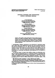
Consider the simple schematic of a reservoir shown in Figure 2-1, where the cost function is cumulative oil production and the control is the injection rate. Changing the

17

injection rate changes the dynamic states of the system (pressures, saturations), which changes the oil production rate, which in turn impacts the cost function. Thus, the controls u are related to J ( u ) through the dynamic system. The dynamic system can also be thought of as a set of constraints that determine the dynamic state given a set of controls. Further, the controls u themselves may be subject to other constraints that dictate the feasible or admissible values of the controls, such as surface facility constraints or fracture pressure limits. It is these additional constraints that in many cases complicate the problem and the solution process. In this chapter, only linear constraints on u will be considered. Nonlinear constraints will be discussed in detail in Chapter 5. The existing optimization algorithms can be broadly classified into two categories: stochastic algorithms like Genetic Algorithms [24] and Simulated Annealing [25], and gradient based algorithms like Steepest Descent [26] and Quasi-Newton algorithms [26]. The first category usually requires many forward model evaluations and does not guarantee monotonic minimization/maximization of the objective function, but is capable (in theory) of finding the global optimum with a sufficiently large number of simulation runs. On the other hand, the second category is generally very efficient, requires few forward model evaluations and also guarantees reduction of the objective function at each iteration, but only assures local optima for non-convex problems [26]. For practical problems, where the simulation grid can be of the order of 106 cells, a single evaluation of the forward model may take many hours; implying that gradient based algorithms would be preferable for such problems. Furthermore, gradient-based algorithms might also be sufficient for the production optimization problem, as any increase in the objective function above the initial manually engineered model is always beneficial. In other words, finding a global optimum may not be necessary – the goal is to determine an operational scenario that represents an improvement over what would otherwise be done.

18

In order to use gradient-based optimization algorithms, the main requirement is an efficient technique to calculate the gradients of the cost function with respect to the controls. Since the dynamic system is too complicated to calculate the gradients analytically, the simplest approach is to approximate the gradients numerically. This method is very easy to implement, as the forward model is treated as a black box. However, doing so essentially renders the whole process highly inefficient, particularly in the presence of a large number of controls and updates, as one forward model evaluation (simulation) is required for each gradient to be calculated. In particular, considering the simple model mentioned before, in order to calculate the gradient of cumulative oil production with respect to water injection rate at a given time t, the injection rate over a time dt is perturbed slightly, and the model is evaluated again. The perturbation results in a perturbation of the oil rate (Figure 2-2) and therefore of the cumulative oil production, and the gradient is calculated with the simple forward difference formula as: ∂J ( u ) ∂u

J ( u + du ) − J ( u ) du

Figure 2-2 Perturbation of injection rate from numerical gradient calculation

Thus, if the set of controls consists of any well variable such as rate or BHP, then the total number of controls would be the product of the total number of wells and the

19

total number of control updates in time (control steps). As seen in Table 2-1, this number can be very large even for a moderate number of wells and control steps. Another issue with this approach is the selection of the magnitude of each perturbation.

Table 2-1 Number of model evaluations for gradient calculation with numerical approximation and optimal control theory (from Brouwer [5])

This chapter explores the application of adjoint models for efficient production optimization through the efficient calculation of gradients. Of the few existing methods for calculating gradients, adjoint techniques are the most efficient, especially for a large number of controls, as the algorithm is independent of the number of controls. However, the complexity of the adjoint calculations is similar to that of the forward simulation, which is one of the main drawbacks of the algorithm, and is also likely one of the primary reasons why adjoint methods have not gained greater popularity in the petroleum industry. There have been some investigations directed toward the use of (adjoint-based) optimal control for production optimization. Ramirez and coworkers have used it to optimize surfactant flooding [27], carbon dioxide flooding [28] and steam flooding [29]. Zakirov et al. [30] have used adjoint models to optimize production from a thin oil rim. Optimization of waterflooding using adjoints has been studied by many researchers including Asheim [31], Virnovsky [32], Sudaryanto and Yortsos [33], and recently by Brouwer and Jansen [5, 34]. In all of

20

these investigations, the major emphasis was on the results of the optimization process, rather than on the algorithm itself. Further, in some of the above papers, the forward model (simulator) used was highly simplified [31, 32] or even analytical in nature [33]. Also, almost all of the above studies lack the implementation of nonlinear constraints on the controls themselves, while, in practical production optimization problems, the optimization process is almost always subject to many nonlinear constraints on the controls. In this chapter, we investigate an adjoint construction procedure that makes it relatively easy to create the adjoint and has the additional advantage of making the adjoint code quite independent of the forward code. Note that the basic idea behind this approach has been known in the petroleum industry for quite some time, for example, Zakirov et al. [30] allude briefly to the idea, although without any detailed discussion of the steps necessary for its implementation. Li et al. [35] also discuss the idea in the context of the history matching problem. In this chapter, we discuss the procedure at a greater level of detail compared to Zakirov et al., with emphasis on its implementation for the production optimization problem. This procedure was implemented within the context of a general purpose research simulator [11]. The current implementation of the algorithm requires the forward model to be fully implicit (the more general case is discussed in the Appendix). Most of the previous investigators have used an IMPES [36] formulation. The performance and practicality of this approach is demonstrated through two examples. 2.1. Mathematical Formulation of the Problem The production optimization problem discussed above requires finding a sequence of control vectors u n (of length m) for n = 0,1,..., N − 1 , where n is the control step index and N is the total number of control steps, to maximize (or minimize) a performance measure J ( u 0 ,..., u N −1 ) . The optimization can be described very generally with the

following mathematical formulation:

21

max J = φ ( xN ) + n

N −1

u

subject to: g n (x n+1 , x n , u n ) = 0 x0 = x0

n=0

Ln ( x n +1 , u n ) ∀n ∈ ( 0,.., N − 1)

∀n ∈ ( 0,.., N − 1) (Initial Condition)

Au ≤ b

∀n ∈ ( 0,.., N − 1)

LB ≤ u n ≤ UB

∀n ∈ ( 0,.., N − 1)

n

Here, x n refers to the dynamic states of the system, such as pressures, saturations, compositions etc. The cost function J consists of two terms. The first term φ is only a function of the dynamic states of the last control step; in an application it could represent, for example, an abandonment cost. The second term, which is a summation over all control steps, consists of the kernel Ln known as the Lagrangian in control literature [37]. For our purposes, it could include the oil and water rates or some function of the saturations (for sweep efficiency). Since Ln usually consists of well parameters or quantities that are functions of well parameters, it is written here in a fully implicit form. The set of equations g n together with the initial conditions define the dynamic system, which are basically the reservoir simulation equations for each grid block at each time step: g n ( x n +1 , x n , u n ) = Accumulation − Flux − Well

The last two equations of Equation (2.2) refer to the additional constraints for the controls, that is, linear constraints and bounds on controls. These are handled directly by the standard constrained optimization algorithm applied in the following examples. Nonlinear constraints (not shown in Equation (2.2)) are much more difficult to satisfy and a method to honor them will be discussed in Chapter 5. Note that in the above formulation of the problem, the control steps and the actual time steps of the simulator

22

are considered equivalent, and the derivations below are based on this assumption. This is however, not usually the case, and the number of time steps is generally greater than the number of control steps. The modifications necessary to handle the more general problem when the time steps and control steps are not the same are discussed at the end of the next section. 2.2. Gradients with the Adjoint Model It was stated earlier that the gradients of the cost function with respect to the controls could be calculated very efficiently using the adjoint equations. The adjoint model equations are obtained from the necessary conditions of optimality of the optimization problem defined by Equation (2.2). These necessary conditions of optimality are obtained from the classical theory of calculus of variations. For a relatively simple treatment of this subject, refer to Stengel [37]. A more detailed and rigorous analysis of the problem and generalization to infinite dimensional problems in arbitrary vector spaces is given by Luenberger [38]. The essence of the theory is that the cost function of Equation (2.2) along with all the constraints can be written equivalently in the form of an augmented cost function given by Equation (2.4).

J A = φ xN +

N −1 n=0

Ln ( x n +1 , u n ) +

T0

(x

0 0 −x )+

N −1

T ( n +1)

n=0

g n ( x n +1 , x n , u n )

For the moment, only the simulation equations are considered. Treatment of the other constraints is discussed later. The vectors

n

are known as Lagrange multipliers,

which can be thought of as elements of the dual space of the vector space to which u n belongs. One Lagrange multiplier is required for each constraint with which the cost function is augmented. That is, the total number of Lagrange multipliers is equal to the product of the number of dynamic states and control steps. For example, if we have a two-phase black oil model with 3000 grid blocks and 400 control steps, the number of Lagrange multipliers is equal to 2×3000×400 = 2.4×106.

23

For optimality of the original problem as well as the augmented cost function, the first variation (or Frechet differential [38]) of the augmented cost function must equal zero. The first variation of J A is given by:

δ JA = +

∂φ ∂x N −1 n =1

∂LN −1 + ∂x N

+ x=x

N

∂Ln −1 + ∂x n

T ( n +1)

TN

N −1 ∂g N −1 N + gn δ δ x N ∂x n =0

∂g n + ∂x n

Tn

T ( n +1)

N −1 ∂g n −1 ∂Ln n δx + + n ∂x n n = 0 ∂u

+ ( x0 − x0 ) δ T ( n +1)

T0

∂g n δ un n ∂u

We observe that the total variation is a sum of the variations of x n , u n and

n

. Since

these variations are independent of one another, each of these terms must vanish for optimality [37, 38]. The g nδ

T ( n +1)

and ( x 0 − x 0 ) δ

T0

terms are zero by definition.

The terms involving δ x n can be made to vanish by choosing

Tn

TN

∂Ln −1 =− + ∂x n ∂φ =− ∂x

T ( n +1)

x=x N

∂g n ∂x n

∂LN −1 + ∂x N

∂g n −1 ∂x n ∂g N −1 ∂x N

n

such that:

−1

∀n = 1,..., N − 1 −1

(Final Condition)

Equation (2.6) is known as the adjoint model. We notice that the Lagrange multipliers n

depend on

n+1

. Thus the Lagrange multipliers for the last control step must be

calculated first according to the second equation above. It is for this reason that the adjoint model is solved backwards in time. With the Lagrange multipliers calculated in this manner, Equation (2.5) reduces to the following:

δ JA =

N −1 n=0

∂Ln + ∂u n

T ( n +1)

∂g n δ un n ∂u

Thus the required gradients of the cost function with respect to the controls are given as:

24

dJ dJ A ∂Ln = = + du n du n ∂u n

T ( n +1)

∂g n ∂u n

∀n ∈ (0,...., N − 1)

If these gradients are zero for some value of u n , then optimality has been achieved with respect to u n , otherwise, these gradients could be used with any iterative gradient-based algorithm to determine the new search direction. The basic steps required for gradient-based optimization with adjoints are summarized as follows: 1. Solve the forward model equations for all time steps with given initial condition and initial control strategy. Store the dynamic states at each time step. 2. Calculate the cost function with results of the forward simulation. 3. Solve the adjoint model equations using the stored dynamic states to calculate the Lagrange multipliers with Equation (2.6). 4. Use the Lagrange multipliers to calculate the gradients using Equation (2.8) for all control steps. 5. Use these gradients with any optimization algorithm to choose new search direction and control strategy. 6. Repeat process until optimum is achieved, that is, all gradients are close enough to zero. It is clear that one forward model evaluation and one adjoint model evaluation is required to calculate the gradients of the cost function, irrespective of the number of controls. The time required to solve the adjoint model is of the same order of magnitude as the forward simulation. Thus with this process, a time equivalent to approximately two simulations is all that is required to calculate any number of gradients (Table 2-1). This is why adjoint-based algorithms can be very efficient, and can potentially lead to huge time savings if the number of controls is large.

25

In the more general case when the time steps and control steps are not equivalent, that is, there is more than one time step in each control step, the production optimization problem can be formulated as follows:

max J= m

u

N −1 N m −1 m = 0 n =0

Lm ,n ( x m, n +1 , u m ) ∀m ∈ ( 0,.., N − 1)

subject to:

∀m ∈ ( 0,.., N − 1)

g m, n (x m, n+1 , x m ,n , u m ) = 0

n ∈ ( 0,.., N m − 1)

x 0,0 = x 0,0

(Initial Condition)

∀m ∈ ( 0,.., N − 1)

Au m ≤ b

∀m ∈ ( 0,.., N − 1)

LB ≤ u m ≤ UB

Here, m is the control step index, and n is the time step index within each control step, and N m is the number of time steps in control step m. Note that the φ term has been removed from the objective function for simplicity. The adjoint equations are given as:

Tm, n

∂Lm,n −1 =− + ∂xm,n

T m, Nm

T m, n +1

∂Lm, Nm −1 =− + ∂xm, Nm

∂g m,n ∂xm,n

T m +1,1

∂g m,n −1 ∂xm,n

∂g m+1,0 ∂xm, Nm

−1

∀n = 1,..., N m − 1, m = 0,..., N − 1

∂g m, Nm −1 ∂xm, Nm

−1

∀m = 0,..., N − 1 (Final Cond.)

We see from the above that there is a final condition at the end of each control step with this formulation corresponding to the last time step of the control step, and this is obtained from the solution of the adjoint system of the first time step of the next control step. The gradients of the cost function with respect to the controls are finally given as: N m −1 dJ ∂Lm, n = + du m n =0 ∂u m

26

T m , n +1

∂g m ,n ∂u m

∀m ∈ (0,...., N − 1)

Note that the following identities hold in the context of the above nomenclature: x m , N m = x m +1,0 ;

m +1,1

=

m , N m +1

This formulation is the actual implementation of the algorithm that is used for the examples demonstrated below. 2.3. Modified Algorithm for Adjoint Construction Despite the great efficiency of the adjoint algorithm, a major drawback of the approach is that an adjoint code is required in order to apply the algorithm. The complexity of the adjoint equations is similar to that of the forward model [39]. Since in our case the forward model is the reservoir simulator, it is understandable why adjoint models have not gained popularity in the petroleum industry. We discuss a modified approach to constructing the adjoint that makes it relatively easy to create the adjoint code. The approach is possible due to certain properties of the fully implicit simulation code (in the current implementation) and the specific forms of the cost function used for production optimization. The main ingredients of the adjoint equations given by Equation (2.6) are the two Jacobians of the simulation equations: ∂g n ( x n +1 , x n , u n ) ∂x n

;

∂g n −1 ( x n , x n −1 , u n ) ∂x n

Of all the terms comprising the adjoint equations, these are the most difficult terms to calculate, as they are functions of the simulation equations. Now, during the forward simulation, at each time step (assume time step = control step for the moment), we solve Equation (2.14) to determine x n+1 . g n ( x n +1 , x n , u n ) = 0

27

Since these equations are nonlinear with respect to x n+1 , the usual method to solve them is through the Newton-Raphson algorithm [36]:

∂g n ∂x n +1

x n+1 = x n+1,k

(x

n +1, k +1

− x n +1,k ) = − g n ( x n +1,k , x n ,k , u n )

Here, k is the iteration index of the Newton-Raphson algorithm at a given time step. At convergence of the algorithm, we observe that the Jacobian used is the same as the second Jacobian appearing in Equation (2.13). In order to obtain the first Jacobian given in Equation (2.13), consider the general form of the fully implicit mass balance equations: g n ( x n +1 , x n , u n ) = F n ( x n +1 ) + W n ( x n +1 , u n ) −

1 An +1 ( x n +1 ) − An ( x n ) n ∆t

Here F refers to the flux terms, W refers to the source terms and A refers to the accumulation terms. Thus the first Jacobian of Equation (2.13) is given as: n n ∂g n 1 ∂A ( x ) = ∂x n ∆t n ∂x n

Now, consider the mass balance equations of the previous time step: g n −1 ( x n , x n −1 , u n −1 ) = F n −1 ( x n ) + W n −1 ( x n , u n −1 ) −

1 An ( x n ) − An −1 ( x n −1 ) n −1 ∆t

The second Jacobian for this time step is given by: ∂g n −1 ∂F ( x = ∂x n ∂x n n −1

n

) + ∂W ( x , u ) − n −1

n

∂x n

n −1

n n 1 ∂A ( x ) ∆t n −1 ∂x n

The last term of Equation (2.19), scaled with ∆t of the two time steps, is the same as the RHS of Equation (2.17). Thus the first Jacobian of any given time step is

28

calculated during the computation of the second Jacobian of the previous time step. The rest of the terms constituting the adjoint equations are relatively easy to calculate, as they are functions of the scalar cost function. In fact, if the cost function can be written in the following manner:

J=

N −1 n =0

Ln ( u n , W n , ∆t n )

That is, it is directly a function of the well terms of the simulation equations rather than a function of the dynamic states, then:

∂Ln −1 ∂W n −1 ∂φ f = ; =0 n n ∂x ∂x ∂x N The first term is a function of the converged well term derivatives with respect to dynamic states at each time step. This is also calculated within the forward simulation as seen from Equation (2.19) and is relatively easy to extract. An example of a cost function of the form of Equation (2.20) is net present value given by the following equation (see the Nomenclature for definition of symbols): Ln ( u n , W n , ∆t n ) =

NP

Pop

j =1

ρ o , SC

Won, j −

Cwp

ρ w, SC

Wwn, j

∆t n

(1 + α )

tn

−

NI j =1

n Cwi qwi ,j

∆t n

(1 + α )

tn

Thus we see that all the terms required for calculating the Lagrange multipliers through the adjoint model can be calculated during the forward model evaluation itself. Furthermore, if NPV is the cost function, and BHP or rates are the controls, then the terms of Equation (2.8) can also be extracted from the forward run: n ∂Ln ∂g n ∂W n n ∂W = f u , n ; = ∂u n ∂u ∂u n ∂u n

29

Therefore, the algorithm for gradient-based optimization using adjoints is modified as follows: 1. Solve the forward model equations for all time steps with given initial condition and initial control strategy. 2. Store the two Jacobians of the simulation equations and the well derivatives at each time step. 3. Calculate the cost function with results of the forward simulation. 4. Solve the adjoint model equations using the stored Jacobians and well derivatives with respect to dynamic states to calculate the Lagrange multipliers with Equation (2.6). 5. Use the Lagrange multipliers and stored well derivatives with respect to controls to calculate the gradients using Equation (2.8) for all control steps. 6. Use these gradients with any optimization algorithm to choose new search direction and control strategy. 7. Repeat process until optimum is achieved, that is, all gradients are close to zero. It should be noted that mathematically there is no change in the algorithm, but the adjoint equations become much simpler to code. Specifically, the version of the General Purpose Research Simulator (GPRS) [11] developed at Stanford University and used as the forward simulator in the following examples consists of around 20000 lines of C++ code, whereas the adjoint code consists of only around 500 lines of Matlab code. However, more importantly, this approach allows the adjoint code to remain fully consistent with the forward model code if any changes to the flux terms or accumulation terms are made or new terms reflecting new physics are added to

30

Equation (2.16). This is because the Jacobians are taken directly from the forward model, so any changes made to the simulation equations are reflected in these. For example, suppose a dual porosity model [40] is implemented into the forward simulator. This implies that a new term (the transfer function) is added to the simulation equations, changing g n ( x n +1 , x n , u n ) . No change is required in the adjoint model code, however, as the partial derivatives of the simulation equations with respect to the states and controls are taken directly from the forward simulator. This is a useful algorithmic feature in general, but it is particularly important in a research or development setting where the forward model is updated frequently. Further, the modified approach is slightly more efficient than the standard approach as the Jacobian forming calculations are not repeated but are directly loaded from memory. However, because the Jacobians must be stored with the modified approach instead of the dynamic states, the storage requirement of the modified approach is much larger. The approximate memory requirements can be estimated with the following equation:

Total GB ≈ 1.6 ( N D + 1) N g N c2 N t /108 Here, N D is the number of physical dimensions, N g is the number of grid blocks, N c is the number of components and N t is the number of time steps. For example, if a given problem is a 3D, 3-phase black oil model with 100000 cells and 100 time steps, the total storage requirement is around 6 GB. Note that this is hard disk memory and not RAM memory, as the Jacobians are stored to files in our implementation. 2.4. Case Study – Horizontal Smart Wells The first case is a simple example adapted from Brouwer and Jansen [34] that effectively demonstrates the applicability of adjoint-based optimization to smart well control. The schematic of the reservoir and well configuration is shown in Figure 2-3. The model consists of one horizontal “smart” water injector and one horizontal “smart” producer, each having 45 controllable segments. The reservoir covers an area 31

of 450 × 450 m2 and has a thickness of 10 m and is modeled by a 45 × 45 × 1 horizontal 2D grid. The fluid system is an essentially incompressible two-phase unit mobility oil-water system, with zero connate water saturation and zero residual oil saturation. Figure 2-4 shows the heterogeneous permeability field with two high permeability streaks running from the injector (left) to the producer (right). The contrast in permeability between the high permeability streaks and the rest of the reservoir is around a factor of 20-40, and it is this heterogeneity that makes the optimization results interesting.

Figure 2-3 Schematic of reservoir and wells for Example 1 (From Brouwer and Jansen [34])

For purpose of optimization, the injector segments are placed under rate control, and the producer segments are under BHP control. There is a total injection constraint of 2700 STB/day (STBD); thus the optimization essentially results in a redistribution of this water among the injection segments. Further, there are also bounds on the minimum and maximum rates allowed per segment, and also bounds on the BHPs of the producers, which could for example correspond to bubble point pressures or fracture pressures. The model is produced until exactly one pore volume of water is injected, which corresponds to around 950 days of injection. This time period is divided into five control steps of 190 days each. Thus the total number of controls is 32

equal to (45+45) × 5 = 450. All constraints in this problem are linear with respect to the controls.

Figure 2-4 Permeability field for Example 1 (From Brouwer and Jansen [34])

In order to understand the benefit of any optimization process, it is usual to compare the optimization results against a base or reference case. In the case of production optimization, such a base case would be a reasonable production strategy that an engineer might devise given a simulation model and a set of constraints. It is, however, very difficult (and often nonintuitive) to understand the implications of varying well controls on the optimization process. It is thus usual for engineers to specify constant production/injection rates or BHPs until some detrimental reservoir response such as water breakthrough is observed. For this case study as well, the base case is kept quite simple. For the purpose of this case study, the base case is a constant rate/constant BHP production strategy. The 2700 STBD of injection water is distributed among the 45 injection segments according to their kh (permeability × pay thickness), which

33

corresponds to an uncontrolled case. The producer BHPs are set in such a way that a balanced injection-production is obtained.

Figure 2-5 Final oil saturations after 1 PV injection for reference case

The objective of the optimization process is to maximize NPV as given in Equation (2.22). The NPV discounting factor is set to zero, meaning that the effect of discounting is neglected. Thus, maximizing NPV is essentially maximizing cumulative oil production and minimizing cumulative water production. The oil price is conservatively set at $80/m3, water injection costs at $0/m3, and water production costs at $20/m3 [34]. It should be noted that it is relatively easy to vary these cost/prices with time and even to implement uncertainty models for them, provided of course that such models can be inferred. Starting from 100% oil saturation throughout the reservoir, Figure 2-5 and Figure 2-6 show the final oil saturations for the uncontrolled and the optimized case after exactly 1 PV of water has been injected. It is clear that the optimization leads to a huge improvement in the sweep efficiency, leading to the increase in NPV of around 100%.

34

Note that the final oil saturations maps obtained are very similar to those obtained by Brouwer and Jansen [34].

Figure 2-6 Final oil saturations after 1 PV injection for optimized case

The reasons behind the better sweep in the optimized case can be easily explained by analyzing the optimized trajectories of the controls – rates/ BHPs of the injectors and producers – as seen in Figure 2-7 and Figure 2-8. The y-axis of Figure 2-7 corresponds to 45 injector segments and the x-axis corresponds to the 5 control steps. The color scale corresponds to injection rates of the segments, with blue being lowest rates (almost closed) and brown being highest (fully open). It is obvious that the injector segments completed in or near the high permeability streaks are shut down at early time, as they force water to move very quickly toward the producers, resulting in early breakthrough and thus poor sweep. Further, some of the injector segments completed in the lower streak tend to open up towards the later control steps, so that the water front between two streaks actually moves laterally (Figure 2-9) towards the streaks, resulting in the almost 100% sweep of this region.

35

Figure 2-7 Injection rate variation with time for optimized case (x-axis represents the control steps, and y-axis represents the 45 injector segments)

Figure 2-8 Producer BHP variation with time for optimized case (x-axis represents the control steps, and y-axis represents the 45 producer segments)

In Figure 2-8, the color scale corresponds to the BHPs of the producer segments, and we again observe that the producer segments completed in or near the high

36

permeability streaks are shut most of the time. Also, the producer segments in between the streaks again open towards the later control steps, so that the water present in the streaks moves toward this region leading to a better sweep.

Figure 2-9 Lateral movement of water in optimized case

Figure 2-10 shows the field water injection rate, the oil production rate and the water production rate for the base case and optimized case. In the optimized case, for most of the time, the oil production rate is significantly higher and the water production lower than the base case. The four peaks in the oil rate correspond to the start of the control steps. Because the actual time steps are smaller than the control steps, the oil or water production rate over a control step does not remain the same. It is interesting to note that although the final saturation map and increase in NPV are quite close to that obtained by Brouwer and Jansen [34], the optimal trajectories of the controls are somewhat different. These differences may be caused by the different control variables used on wells, slightly different fluid compressibilities, or different lengths of control steps, or it may be that the local optima obtained are different, but with similar values of the optima. 37

Figure 2-10 Comparison of total production rates for reference and optimized case

Figure 2-11 Comparison of cumulatives for reference and optimized case

Figure 2-11 shows that there is a substantial increase in cumulative oil production (70%), attributed to the better sweep, and a slight decrease in water production (6%) after the optimization process. The optimization process required five iterations of the optimization algorithm (Sequential Quadratic Programming from the Matlab Optimization Toolbox [41]); the total number of simulations required for the optimization was around 12-15.

38

2.5. Case Study – SPE 10 Layer 61 This example is a more complex case adapted from the 10th SPE Comparative Solution Project [42]. The model is described on a regular Cartesian grid. The model dimensions are 1200 × 2200 × 170 (ft). The top 70 ft (35 layers) represents the Tarbert formation and the bottom 100 ft (50 layers) represents Upper Ness formation. The cell size is 20 ft × 10 ft × 2 ft. The model has 60 × 220 × 85 cells and consists of part of a Brent sequence. For this case study, only layer 61 belonging to the Upper Ness fluvial formation is selected. The highly heterogeneous permeability field for this layer is shown in Figure 2-12.

Figure 2-12 Permeability field for SPE 10 Layer 61

The fluid system is a two-phase oil water system with low compressibility and a very unfavorable mobility ratio (≅ 75). The relative permeabilities are the usual Corey type curves. The production model is a five-spot pattern with a vertical injector at the center and four vertical producers at the corners. Thus there are two drive mechanisms: depletion drive and water injection. The injector is under rate control and the producers are under BHP control. The reference case is again a constant rate/BHP case, with the injection rate set at 5000 STBD and all producer BHPs at 3000 psi. The injection rate is constrained at a maximum of 6000 STBD and the producer BHPs at a minimum of 500 psi and a maximum of 4000 psi. These are linear constraints with respect to the controls.

39

The objective is to maximize the NPV over a period of 4.5 years, divided into control periods of 30 days. Thus the total number of controls is equal to 5×55 = 275. The NPV discounting factor is again set at zero, meaning that the effect of discounting is neglected. The oil price is conservatively set at $30/Bbl and water injection costs at $3/Bbl. The case is made interesting by making it extremely expensive to process produced water, and the water production cost is set at $40/Bbl. Although this high water production cost is unrealistic in most settings, it makes the optimization process more complex and different from the first case, as the optimization must here reduce water production, even at the cost of reducing oil production.

Figure 2-13 Comparison of injection rates for reference and optimized case

Figure 2-13 compares the injection rate of the optimized case to that of the reference case. There is a substantial decrease in injection rate as expected. Due the extremely high water production costs, water injection is reduced so that water production may be reduced. However, in order to maintain the oil production rate, all of the producers except PROD 1 produce at around the minimum BHP (Figure 2-14), that is, they are fully open. The main drive mechanism thus changes from water injection in the reference case to depletion drive in the optimized case. PROD 1 on the other hand is producing the maximum amount of water in the reference case as seen in Figure 2-15.

40

Thus, in the optimized case, instead of a reduction of BHP, in an attempt to curtail the high watercut, the BHP of PROD 1 increases, and in fact goes towards the maximum allowed BHP at the end of the run (Figure 2-14).

Figure 2-14 Comparison of BHPs of producers for reference and optimized case

Figure 2-15 Comparison of watercuts for some producers for reference and optimized case

41

Figure 2-16 compares the cumulative water injection, oil production and water production of the base case and optimized case. It is clear that the increase in NPV (by 200%) is due to the huge reduction in water injection (67%) and production (19%), while the cumulative oil production is not much reduced (11%). It is interesting to compare the final oil saturation maps for the reference and optimized case, as seen in Figure 2-17 and Figure 2-18. Unlike the previous case, the optimization results in a decrease of the overall sweep, as the water injected is much less, but the channels leading to PROD 2 and PROD 4 show a slightly better sweep, implying that the injected water is distributed more evenly compared to the reference case.

Figure 2-16 Comparison of cumulatives for reference and optimized case

Figure 2-17 Final oil saturation map for reference case

42

Figure 2-18 Final oil saturation map for optimized case

The number of iterations of the Sequential Quadratic Programming [41] algorithm required for the above optimization was 10, which corresponds to around 25-30 simulation runs. Average run time for one simulation on a 2.8 GHZ machine with 4 GB RAM was around 10 minutes, and the total optimization time was around 5.7 hours. 2.6. Summary This chapter demonstrated the application of adjoint models for the efficient calculation of gradients. A modified approach for the construction of the adjoint model was also described, provided a fully implicit forward model is available, and the cost function can be cast into certain forms. It was shown that the modified approach makes it relatively easy to code the adjoint as compared to the standard approach. Further, another important advantage of this technique is that the consistency between the adjoint code and the forward model code is automatically maintained if any changes to the flux terms or accumulation terms are made or new terms reflecting new physics are added to the forward model. Two dynamic waterflood examples were discussed demonstrating the practicality and efficiency of the approach.

43

Chapter 3 3. Adjoint-based Optimal Control and Model Updating As discussed in the first chapter, the closed-loop approach for efficient realtime optimization consists of three key components: efficient optimization algorithms, efficient model updating algorithms, and techniques for uncertainty propagation. In this chapter, we discuss a gradient-based model updating technique, and combine it with the optimal control algorithm presented in the last chapter to obtain a simplified implementation of the closed-loop approach. Uncertainty propagation is not considered here. Neglecting uncertainty propagation essentially means that the closedloop process is applied to a single realization of the uncertain parameters; e.g., the maximum likelihood estimate, which is updated at every control step. Such a procedure can be expected to provide near-optimal results in many cases, though the treatment of uncertainty will of course be important in many applications. Uncertainty propagation and the entire loop are discussed in Chapter 4. Within the context of closed-loop reservoir management, Brouwer et al. [9] used adjoint models for optimization and Kalman filters for model updating.

Adjoint

models allow for very efficient optimization, although their implementation can be complicated. The ensemble Kalman filter has only recently been applied for history matching [43]. Although this approach is straightforward to implement [43,44], its efficiency compared to established methods like adjoint models may be an issue. Aitokhuehi and Durlofsky [45] used conjugate gradient algorithms with numerical gradients for optimization and the probability perturbation method [46] for model updating. The use of numerical gradients and the stochastic probability perturbation

44

method makes the implementation quite easy, but both algorithms are very expensive computationally, which may limit the use of this procedure in practical settings. In this chapter, we apply the adjoint methods described in the last chapter for the efficient calculation of gradients of the objective function with respect to the controls, which are then used by gradient-based optimization algorithms for the optimization part of the closed-loop. For the model updating procedure, we use Bayesian inversion theory and apply an efficient parameterization of the permeability field using the Karhunen-Loeve (K-L) expansion. This allows us to describe the uncertain parameter field (e.g., permeability), in terms of two-point statistics, using very few parameters. A key advantage of the K-L description is that these parameters can be varied continuously while maintaining the underlying geostatistical description. As a result, adjoint techniques can be applied for the history matching while preserving some degree of geological realism. This procedure is much faster than stochastic algorithms and, unlike standard gradient-based algorithms, implicitly honors the two-point statistics of the geological model. An extension of the K-L procedure described in this chapter which preserves multi-point statistics will be presented in Chapter 6. The use of adjoints for history matching was pioneered by Chen et al. [47] and Chavent et al. [48], who applied it to single-phase problems. Since then, many other researchers have modified and improved the application of adjoint models for multiphase history matching including Wasserman et al. [49], Watson et al. [50], Wu et al. [51], Li et al. [35], Wu and Datta-Gupta [52], and Zhang et al. [53]. Gavalas et al. [15] introduced the use of an eigenfunction expansion for efficient parameterization of reservoir properties, which was also used later by Oliver [54] and Reynolds et al. [55]. This chapter starts with a description of the model updating algorithm. It is then combined with the optimization algorithm of the last chapter in a sequential manner to perform optimization for an uncertain reservoir description. Two variants of the implementation of the model updating algorithm within the closed-loop are discussed. 45

Next, the efficiency and applicability of this approach is demonstrated through a realtime dynamic waterflood optimization of a synthetic reservoir under production constraints and with an uncertain permeability field. The closed-loop optimization methodology is shown to provide a substantial improvement in NPV and sweep efficiency over the base case, and the results are quite close to those obtained with known geology. 3.1. Model Updating as a Minimization Problem A number of techniques are available for the history matching problem. Gradientbased procedures are in general very efficient, but standard implementations suffer from two limitations. First, they tend to find local rather than global minima. Although this is the case to some extent with all history matching algorithms, stochastic optimization techniques introduce a random component to sample the parameter space more broadly. The second limitation inherent in standard gradient-based techniques is that geological constraints are not preserved. This occurs because, during the optimization, geostatistical correlations between model parameters are not maintained. The technique applied here circumvents this latter difficulty by introducing an efficient parameterization of the permeability field in terms of the Karhunen-Loeve expansion (the K-L expansion, described in more detail below, is essentially an eigenfunction expansion) [15, 54, 55]. Because the parameters appearing in the K-L expansion are uncorrelated, any set of these parameters provides a permeability field that honors the underlying two-point geostatistics. Thus, these parameters can be varied in any way to achieve a history match. The technique is much more efficient than stochastic search procedures and has the additional advantage that much of the adjoint code developed for the production optimization problem can also be applied with some modifications to the history matching problem. The model updating component of the closed-loop is a problem of inversion of production data (well pressures and flow rates) in order to determine reliable estimates

46

of uncertain model parameters (porosity and permeability). Within the context of Bayesian inverse modeling, the solution to the general inverse problem consists of combining all prior information as given by the prior probability density of the observed data d , given by ρ D ( d ) , the prior probability density of the model parameters m , given by ρ M ( m ) and the forward model d = f ( m ) to determine the posterior probability density of the model parameters σ M ( m ) given by the following general equation [13]:

σ M (m ) = k ρM (m ) ρD ( f (m ) ) where k is a normalization constant. The most general approach for solving any nonlinear inverse problem involves determining the entire probability distribution

σ M ( m ) , which requires an extensive exploration of the model space, usually accomplished using random search techniques such as a Monte Carlo method [13]. For the case of history matching, however, solving the forward model d = f ( m ) is usually quite time consuming, and in practical cases a single evaluation can take several hours of computation. Therefore we must often be satisfied with the determination of the maximum likelihood and a reasonable estimate of the dispersion of the distribution around it. This is generally accomplished through least-squares techniques, which is a special case of Equation (3.1), when both the prior probability densities ρ M ( m ) and ρ D ( d ) are Gaussian. Under these assumptions, the model updating problem reduces to the minimization of the following misfit function, where C D and C M are the data and parameter prior covariance matrices [13]:

S ( m ) = ( f ( m ) − d obs ) C-1D ( f ( m ) − d obs ) + ( m − m prior ) C-1M ( m − m prior ) T

T

In the general problem of model updating, the forward model d = f ( m ) (simulation equations and outputs) is not only a function of the model parameters m , but is also a 47

function of the dynamic states x (grid pressures, saturations, etc.) and a set of controls

u (well rates, bottom hole pressures etc.), that is: d = f ( x n +1 , u n , m ) , where n is the time step index ( m is assumed to be time invariant). The dynamic states x are functions of both m and u . Thus the mathematical formulation of the general model updating problem is as follows:

min S = ( m − m prior ) C-1M ( m − m prior ) + T

m

subject to: g n (x n+1 , x n , u n , m) = 0 x0 = x0

N −1 n =0

Ln ( x n +1 , u n , m ) ∀n ∈ ( 0,.., N − 1)

∀n ∈ ( 0,.., N − 1) (Initial Condition)

m ∈ Geologically Consistent Realizations The Lagrangian Ln ( x n +1 , u n , m ) has the following form for the history matching problem (assuming that measurement uncertainties are independent):

Ln ( x n +1 , u n , m ) =

Nw

f i n ( x n +1 , u n , m ) − d nobsi

i =1

2

σ in

Here σ in is the standard deviation of the measured data and Nw is the number of wells. The set of equations g n (x n +1 , x n , u n , m ) = 0 together with the initial condition x 0 = x 0 refers to the reservoir simulation equations (forward model) which constrain the dynamic states x . The geological constraints (last set of constraints in Equation (3.3)) are required because production data on its own is not fully constraining. Even with these geological constraints the system is still not fully constrained, but the use of these constraints guarantees that the resulting m will be consistent with the geostatistical description.

48

3.2. Bi-orthogonal Expansions and Adjoints for Updating

As mentioned before, standard gradient-based algorithms will not maintain the necessary geological constraints. As a result, although the objective function might be reduced by a large amount, the final m may not be geologically realistic, which will generally result in poor predictions. By introducing the K-L expansion of the random parameter field m , the problem defined in Equation (3.3) is transformed such that the geological constraints (as defined by the covariance matrix of m ) are implicitly honored. In addition, the number of parameters defining m is decreased significantly, resulting in a greater reduction of the uncertainty envelope compared to the direct solution of the original problem [54, 55]. The Karhunen-Loeve expansion is a very powerful tool for representing stationary and non-stationary processes with explicitly known covariance functions. Any random field or process can be represented as a series expansion involving a complete set of deterministic functions with corresponding random coefficients [56]. This method provides a second-moment characterization in terms of random variables and deterministic functions. The use of K-L expansion with orthogonal deterministic basis functions and uncorrelated random coefficients has generated interest because of its biorthogonality property, that is, both the deterministic basis functions (eigenfunctions) and the corresponding random coefficients are orthogonal. This allows for the optimal encapsulation of the information contained in the random process into a set of discrete uncorrelated random variables. For a random field m ( x, θ ) with a finite variance and a mean m ( x ) , the K-L expansion in continuous form is given as [14]: m ( x, θ ) = m ( x ) +

∞ i =1

λi f i ( x ) ξi (θ )

Here, x is the spatial (or temporal) variable, θ is a random event, ξi (θ ) is a set of uncorrelated random variables, and λi and

f i ( x ) are the eigenvalues and

49

eigenfunctions of the covariance function C ( x1 , x2 ) of m ( x, θ ) . By definition

C ( x1 , x2 ) is bounded, symmetric and positive definite. Following Mercer’s theorem [56], C has the following spectral or eigen decomposition: C ( x1 , x2 ) =

∞ i =1

λi f i ( x1 ) f i ( x2 )

Because reservoir simulation models are defined on discrete grids, we are more interested in the discrete form of the K-L expansion. The truncated K-L expansion of the correlated (geologically constrained) random variables m is given as [56]:

[m ]H ,1 = [ ]H , K [ ]K , K [ ]K ,1 + [m ]H ,1 Here,

is the matrix of the eigenvectors corresponding to the K largest eigenvalues

of the covariance matrix C M ,

is a diagonal matrix consisting of the K largest

standard deviations (square roots of eigenvalues),

is a vector of uncorrelated

standard random variables with zero mean and unit variance (dimension K), and m is the expected value of m . In practice, K i

aij ,2ξiξ j

Here n is the number of random variables used to represent the uncertainty in the model inputs, and the coefficients ai , m , aij ,m are the coefficients to be estimated. Note that the higher the order of the expansion, the better is the approximation. However, the number of unknown coefficients to be determined and therefore the number of collocation points increases quickly as the order is increased. For example, the number of collocation points required for a 2nd order and 3rd order expansion are as follows: 84

N 2 = 1 + 2n + N 3 = 1 + 3n +

n ( n − 1) 2 3n ( n − 1) 2

+

n ( n − 1)( n − 2 ) 6

Step 4: Estimation of Coefficients in Functional Approximation In order to find a good approximation for the model with the fewest number of model runs, it is important to carefully select the parameter values, or collocation points. As noted earlier, the method for selecting collocation points is derived from the same idea as the Gaussian quadrature method to numerically solve integrals [62]. In the collocation method, the points for the model runs are selected from the roots of the next higher order orthogonal polynomial for each uncertain parameter. In general, the number of roots is usually much larger than the number of collocation points required, especially when the number of input random variables is large. The highest probability roots are usually chosen first as the collocation points. For one-dimensional problems, this method gives the same results as Galerkin’s method [18] and hence is regarded as an “optimal method”. Once the P collocation points are chosen, the true model

y = f ( x ) is evaluated P times. Using Equation (4.8) and the P true responses, P linear equations can be derived, which can be solved to obtain the P coefficients aˆ j .

Step 5: Evaluation of Convergence of Approximation Before using the approximation, the convergence of the approximation has to be determined. To check the error of convergence, the model has to be run a few more times, and the model results compared to the approximation results. For the error check model runs, more collocation points are required. These points are derived from the next higher order orthogonal polynomials. The next higher order is used because if the errors are too large and a higher order of approximation is required, we will already have the model solutions needed to solve the approximation.

85

For each of the higher order collocation points, both the true model y = f ( x ) and the approximation y =

P j =0

aˆ jψ j (

)

have to be solved. The convergence error is computed

as:

( y − y )i

2

ε= i

Here, P

( )

P

( i)

is the joint probability density at the corresponding values of the

uncertain parameters. If the error is small enough, the approximation can be used for uncertainty analysis, otherwise, the next higher order approximation is evaluated and the process repeated until convergence is achieved.

Step 6: Use Approximation for Uncertainty Analysis Once a sufficiently accurate approximation has been determined, it can be used for a variety of statistical analyses. For example, a Monte Carlo simulation can be used to obtain the probability density function of y , as the approximation is algebraic and therefore its evaluation very fast. Other information such as the mean or standard deviation is even simpler to obtain. For example, the mean of y is the expected value

E [ y ] , which is just the coefficient aˆ0 of the approximation. This is a result of the use of orthogonal polynomials; the expected value of every other term in y is 0 because they contain products of different order orthogonal polynomials. In fact, for the closedloop application described below, only the mean of y ( y is NPV in the example) is required. The standard deviation is similarly simple to calculate. One problem with the PCM as described above is that the input random variables have to be independent. In the case when the random input properties consist of random fields (a set of spatially distributed correlated random variables) or random processes (a set of temporally distributed correlated random variables), the standard probabilistic

86

collocation method cannot be used directly due to the independence assumption of the input random variables

. This however is usually the case with reservoir simulation

models, whose input parameters such as porosity and permeability of one grid cell are related to those of another grid cell. The Karhunen-Loeve expansion, as explained in the last chapter, allows the expression of a correlated random field or process in terms of a set of independent random variables while maintaining the covariance structure. Thus, once the K-L expansion of the input random field is performed, the PCM can then be performed using the independent random variables obtained with the K-L expansion. Further, the number of transformed independent random variables is much smaller than the initial correlated random variables, which is very beneficial for PCM as the number of collocation points and therefore the efficiency is directly dependent on the number of input variables. Refer to Chapter 3 for a description of the KarhunenLoeve expansion. 4.3. Application of PCM+KLE to a Gaussian Random Field

To demonstrate the validity of the PCM+KLE approach, we consider a multi-Gaussian permeability field (log permeability) with exponential covariance. The correlation length is 3/5 of the spatial dimension of the model, and there is a nugget effect of 0.1. The lognormal permeability distribution has a mean of 100 and standard deviation of 48. The model size is 50×50, that is, the number of correlated random variables (log permeability) is 2500. All other input properties of the reservoir are assumed to be deterministic. The output random variable considered is net present value (NPV). A set of 1000 realizations is created by unconditional simulation using sgsim [63]. Some of the realizations are shown in Figure 4-2. The simulation model is a quarter 5-spot 2D 2-phase black oil model with a water injector under rate control (left bottom corner) and a producer under BHP control (right top corner). The model is run for 900 days. Karhunen-Loeve expansion is performed using the 1000 realizations and the eigenvalues and their energy are plotted in Figure 4-3 and Figure 4-4. We observe that 87

most of the energy is associated with the first few eigenpairs. For the purpose of model updating, we chose to retain only 10 eigenpairs; this corresponds to about 65% of the total energy. The number of independent random variables is thus reduced from 2500 to 10. Note that the fraction of energy associated with a number of eigenpairs is primarily dependent of the correlation lengths and not on the number of grid cells, and therefore, as long as the correlation lengths are sufficiently long, such large reduction in retained eigenpairs should also be possible for large-scale models. Figure 4-5 and Figure 4-6 show the reconstruction of the reference permeability field with the first 10 eigenpairs. As before, it is clear that although the long correlation features are preserved, the smaller correlation structures are lost. However, since flow behavior and therefore NPV is mainly dependent on longer correlation lengths, such an approximation should be reasonable, at least for multi-Gaussian type structures. Realization 1

Realization 2 5.5

10

5

20

4.5

30

4

40 50

3.5 10

20

30

40

50

Realization 3

10

5.5

20

5

3.5 50

10

20

5

20

4.5 4

40

3.5 20

30

10

40

50

20

30

40

50

Realization 4

5.5

10

4

40

10

50

4.5

30

6

30

6

6 5.5 5 4.5

30

4

40 50

3.5 10

20

30

40

50

3

Figure 4-2 A few realizations with Gaussian permeability and exponential covariance

88

Figure 4-3 Eigenvalues of the Covariance Matrix

Since the initial random field (log permeability) is Gaussian, Hermite polynomials can be used directly. A 2nd order expansion is used, and as seen from Equation (4.10), as the number of random variables is 10, 66 collocation runs are required for a 2nd order expansion. Combinations of the roots of the 3rd order Hermite polynomial are used as collocation points according to the rule described earlier. Since an analytical solution is not possible, the validity of the approach is compared against Monte Carlo simulation . In order to determine the number of realizations of permeability required for Monte Carlo, a convergence study of the mean and variance of permeability is performed. Convergence of some of the permeabilities is shown in Figure 4-7. It is observed that the mean and variance of the realizations converge to the true mean and variance (i.e., the mean and variance used to generate the realizations) at around 600 realizations, implying that about this many realizations would be required to obtain a reliable pdf of NPV by a Monte Carlo procedure.

89

Figure 4-4 Fraction of total energy associated with the eigenpairs Original Log(Perm) Field

Rec onstructed Log(Perm) Field

5

5.2

5 5.5

10

10 5

15

15 5

20

4.8

20

25

25 4.5

30 35

4

40

35

4.4

40

45 50

4.6 30

3.5

10

20

30

40

50

4.2

45 50

10

20

30

40

50

Figure 4-5 Original realization 1 and its reconstruction from first 10 eigenvectors

Figure 4-8 compares the pdfs of NPV obtained by Polynomial Chaos and by Monte Carlo. It is clear the PCE pdf is a very close approximation to the pdf obtained by Monte Carlo. However, 66 simulations were required in the case of PCE as compared to 600 for Monte Carlo, demonstrating a significant increase in efficiency. This can be further improved if an adjoint model is also available. Note that the Monte Carlo

90

method used in this work is the most basic one, and more efficient Monte Carlo techniques such as Latin hypercube sampling are also available. Original Log(Perm) Field

Rec onstructed Log(Perm) Field 6

5

5.6

5 5.5

10

5.4

10

5.2 15

15 5

20

5 20 4.8

25

4.5

25 4.6

30

30 4.4

4 35

35 4.2

40

3.5

45 50

40

4

45 3 10

20

30

40

50

50

3.8

10

20

30

40

50

Figure 4-6 Original realization 2 and its reconstruction from first 10 Eigenvectors

Figure 4-7 Convergence of mean and standard deviation of permeability

Table 4-1 compares the mean and variance of NPV obtained from PCE, Monte Carlo and using the 66 collocation points directly (without any polynomial chaos expansion being used). PCE and Monte Carlo display a very good agreement (7% error). Although the 66 collocation points give a reasonable value for the mean, the variance is 35% less than that obtained by Monte Carlo. 91

NPV from PCE

50 45

45

40

40

35

35

30

30

25

25

20

20

15

15

10

10

5

5

0

4

4.5

5

5.5 NPV

NPV from Montecarlo

50

6

0

6.5 x 10

4

4.5

5

5.5 NPV

7

6

6.5 x 10

7

Figure 4-8 NPV distribution from PCE and Monte Carlo

Mean Variance

PCE 5.572e+007 1.632e+013

Monte Carlo 5.548e+007 1.768e+013

Collocation Points 5.593e+007 1.140e+013

Table 4-1 Mean and variance from PCE and Monte Carlo

4.4. Implementation of the Closed-Loop

Before the closed-loop formulation can be completed, the optimization algorithm described in Chapter 2 and the uncertainty propagation algorithm described above must be combined. This is required because, due to the uncertainty of the model parameters, the outputs of the forward model that comprise the objective function of the optimization problem become random variables. Since the objective function is generally required to be a scalar quantity, it usually consists of some moment of the output random variables (such as the expected value) or a combination of different moments [45]. These moments and their gradients with respect to the controls can be calculated directly from the polynomial chaos expansion, provided that the gradients of output variables at the collocation points are available (for example using the deterministic adjoints discussed earlier). Consider for example the approximation of

92

some output y = f ( ξ ) of a forward model with a second order Hermite chaos representation:

y = a0,2 +

n i =1

ai ,2ξi +

n i =1

aii ,2 (ξi2 − 1) +

n −1 n i =1 j >i

aij ,2ξiξ j

Here n is the number of input random variables. If the objective function consists only of the expected value of y , given by E ( y ) , then, since ξ is a set of Gaussian random variables with zero mean and unit variance, E ( y ) = a0,2 , i.e., the first coefficient of the expansion. As explained in the last section, using the solutions at the P collocation points, a linear system can be obtained to determine a0,2 (and the other coefficients if required). The expected value and its gradient can then be written as:

E ( y ) = a0,2 =

P i =1

bi yi ;

dE ( y ) = du

P i =1

bi

dyi du

Here yi and dyi / du are obtained from the collocation runs of the forward model and the adjoint model (at the collocation points). Using Equation (4.13), the expected value and its gradient, as required by the optimization algorithm, can be obtained. The coefficients bi are obtained from the inverse of the matrix containing the Hermite polynomials evaluated at the collocation points [18]. Note that for a second order chaos expansion, the number of collocation runs P, which is equal to the number of coefficients ai1 ..in to be determined, is given by the first equation of Equation (4.10). Interestingly, if we only require the expected value y , then due to the nature of the roots of the third order Hermite chaos, a0,2 is not affected by the ξiξ j terms of Equation (4.12). Thus the number of collocation runs actually reduces to 1 + 2n . This can be further reduced by only considering the larger ai1 ..in coefficients and discarding the rest, as will be demonstrated in the example of the next section. Also, since the number of collocation runs depends on the number of input variables, reducing the

93

number of input variables using the K-L expansion to parameterize a random input field results in further speed up of the uncertainty propagation process. Combining all of the components discussed in this and previous sections, the formulation of the closed-loop can be implemented efficiently. The main steps required to complete the loop are as follows: 1. From the prior model of the uncertain but correlated parameter field, calculate the covariance matrix, either numerically or analytically. Note that the covariance model may be non-stationary. 2. Perform Karhunen-Loeve expansion to determine the eigenvectors and eigenvalues of the covariance matrix. Retain only the largest eigenpairs; the number to be retained can be determined from the percentage of the total energy contained in the eigenpairs. 3. Determine the order and type of the polynomial chaos expansion to be used. Since the K-L expansion is being used for the correlated random field, an assumption of Gaussianity of this input random field has already been made. Thus the Hermite chaos representation should be used for these input random variables. Determine the coefficients bi from the values of the polynomial chaos at the collocation points. 4. Using the current estimate of the controls, evaluate the forward model and the adjoint model at the collocation points from control step k to Nt, (total control steps) starting with k = 1, that is, the first control step. 5. Determine the objective function and its gradient with respect to the controls using the output from step 4 and Equation (4.13) (if the objective function only consists of the expected value of some output of the forward model) or similar equations depending on the nature of the objective function.

94

6. Perform optimization from control step k to Nt, starting with k = 1, that is, the first control step, to determine the new controls. 7. Apply the optimized trajectory of the controls on the “true” reservoir from control step k to k+1, and record the reservoir response for this time period. This provides the “data” to be used for history matching. 8. Perform model updating to assimilate new data. Updating can be performed from control step 1 to the step k+1, that is, assimilate new data and re-assimilate earlier data, or from step k to k+1, that is, only assimilate new data. 9. Perform steps 4 to 8 for the next control step, (k=k+1) using the new maximum likelihood estimate of the parameter field and its posterior covariance to obtain the new collocation realizations. Repeat until k= Nt. Further discussion of some of the above steps (specifically those associated with model updating) is provided in Chapter 3. In addition, it should be noted that along with the input correlated random field, there might also be other independent input random variables of the forward model. For example, in the application demonstrated below, the permeability field is assumed unknown and is therefore the input random field. But, we may also have other unknowns such as the depth of the water-oil contact that are independent of the permeability field. These random variables can also be directly incorporated into the polynomial chaos expansion in addition to the random variables related to the K-L expansion of the correlated random field.

4.5. Case Study – Dynamic Waterflooding Application of the closed-loop approach is demonstrated on a simple dynamic waterflooding example with smart wells. This example was also considered in Chapter 3; the new element here is the incorporation of uncertainty propagation via polynomial chaos expansions. Thus, much of the description below follows that in Chapter 3. Further, in Chapter 3 we discussed two approaches for model updating. Here we apply

95

the second such approach in which only new data (rather than all of the historical data as in the first approach) is assimilated at every control step.

Figure 4-9 Magnitude of the coefficients of the polynomial chaos expansion

Since the simulation model is the same as in Chapter 3, it will not be discussed here. Again, permeability is assumed to be unknown and will be updated by assimilating production data. Prior knowledge of the reservoir is depicted by the training image [57] shown in Figure 3-1, with the channel sand permeability being about 10 Darcy and the background sand permeability about 500 mD. Realization 22 from Figure 3-2 is taken to be the true realization. Karhunen-Loeve expansion is performed using the covariance matrix created from 1000 initial realizations. For the purpose of model updating and uncertainty propagation, we chose to retain only 20 eigenpairs; this corresponds to about 68% of the total energy of the eigenpairs. The production scenario is also the same as in the example from Chapter 3. There is a total injection constraint of 2700 STB/day (STBD). The model is produced until exactly one pore volume of water is injected, which corresponds to around 950 days of

96

injection. This time period is divided into seven control steps of 30, 60, 100, 190, 190, 190 and 190 days. Thus the total number of controls is equal to (45 + 45)×7 = 630. These seven control steps also correspond to the model updating steps. The injection BHPs and producer water and oil rates from the “true” model are used as data to update the permeability field. The base case is again a constant rate/constant BHP production strategy. The 2700 STBD of injection water is distributed among the 45 injection segments according to their kh, which corresponds to an uncontrolled case. The producer BHPs are set in such a way that a balanced injection-production is obtained. The key difference from Chapter 3 is that NPV is now treated as a random variable. Thus, the objective of the optimization process is to maximize the expected value of NPV with discounting factor set to zero. The oil price is conservatively set at $80/m3, water injection cost at $0/m3, and water production cost at $20/m3. To perform uncertainty propagation, a second order Hermite chaos is chosen to represent NPV. As there are 20 input random variables (from the K-L expansion), and we are only interested in the expected value of NPV, the number of coefficients to be determined is equal to 41 (from Equation (4.10)). The magnitude of these coefficients calculated using the uncontrolled case is shown in Figure 4-9. We observe that most of the coefficients are quite small in magnitude, and can thus be eliminated without affecting the calculated NPV significantly. Using a cutoff of ± 0.4e6 (red lines in Figure 4-9), the number of coefficients is reduced to 9. This is the number of collocation runs that is required to calculate the expected value of NPV and its gradient (with the adjoint). Note that as the controls change during the optimization, the forward model that the Hermite chaos represents also changes, and thus the ranking (in magnitude) of the 41 coefficients may not remain the same, implying that the coefficients to be discarded may change. Retaining these particular 9 coefficients is thus based on the assumption that the change in the forward model does not affect the ranking of the coefficients. This issue requires further investigation. 97

Figure 4-10 Permeability field updates obtained with the closed-loop approach with uncertainty propagation

98

Figure 4-11 Final oil saturations obtained with the closed-loop approach with uncertainty propagation

Figure 4-12 Comparison of cumulative production for base (uncontrolled) case and optimized case (OPTIM_TRU) run with “true” realization, and closed-loop with (OPTIM_CL2) and without (OPTIM_CL1) uncertainty propagation

99

Figure 4-10 and Figure 4-11 show the maximum likelihood models and final saturation map obtained using the complete closed-loop with uncertainty propagation. Again, as in the simplified closed-loop of Chapter 3, the sweep obtained is almost as good as with the open loop, and in this case the sweep patterns are also very similar. This is due to the fact that the maximum likelihood estimates of the permeability field (Figure 4-10) provide reasonable optimization trajectories. This is also evident in the cumulative production profiles of Figure 4-12, where the production profiles obtained with the complete closed-loop follow the profiles obtained from the optimization on the true field very closely. Although the final NPV obtained at 950 days is very close for both closed-loop approaches (around 25% over reference), the loop with uncertainty propagation clearly displays better performance for the time period before about 750 days.

4.6. Summary We have demonstrated that adjoint models combined with bi-orthogonal expansions, in particular K-L and Hermite expansions, can be used for efficient uncertainty propagation and closed-loop optimal control. Significant improvements in recovery appear to be possible through the application of such techniques. In particular, the following may be concluded: 1. Polynomial chaos expansions may be used for efficient uncertainty propagation, with the main benefit that standard deterministic forward models and associated adjoints can be used as in a black box approach. 2. For the example considered, the increase in NPV and sweep efficiency by the closed-loop approach is very close to that obtained using an open-loop approach. In addition, the results indicate that approximate parameter fields may be adequate for obtaining near optimal trajectories of the controls.

100

3. Including uncertainty propagation within the closed-loop results in more reliable estimates of the optimal trajectories, as opposed to a closed-loop applied only on the maximum likelihood estimate of the uncertain parameter field. A few additional issues concerning the polynomial chaos and Karhunen-Loeve expansions need to be addressed. We need to explore whether preserving two-point statistics is sufficient for the purpose of optimal control under complex geological scenarios. Further, the optimal order of polynomial chaos to be used, and the number of terms to be retained, is yet to be fully understood. Some of these issues will be addressed in later chapters.

101

Chapter 5 5. Handling Nonlinear Path Inequality Constraints This chapter is focused on the optimization component of the closed-loop process with emphasis on handling nonlinear path inequality constraints. This problem can essentially be cast as a large-scale path constrained optimal control problem. A large variety of methods for solving discrete-time optimal control problems now exist in control theory literature, including dynamic programming, neighboring extremal methods, gradient-based nonlinear programming methods (NLP), etc. These are discussed in detail in Stengel [37] and Bryson and Ho [20]. Of these approaches, the NLP method combined with the Maximum Principle [20] (adjoint models) generates a class of NLP methods in which only the control variables are the decision variables and the state variables are obtained from the dynamic equations. These algorithms are generally considered more efficient compared to the other methods. Further, within this class of NLP methods, there are many existing techniques available for handling nonlinear control-state path inequality constraints [20, 64, 65, 66]. However, as will be discussed later, these are either not practical for the production optimization problem or are difficult to implement with existing reservoir simulator codes. In petroleum engineering literature, papers by various authors such as Asheim [31], Vironovsky [32], Brouwer and Jansen [34], etc. have discussed the application of adjoint models and gradient techniques for the production optimization problem in significant detail. However, an important element that is missing from most of these papers is the effective treatment of nonlinear control-state path inequality constraints (for example, a maximum water injection rate constraint). Such constraints are always present in practical production optimization problems, and therefore their efficient treatment is essential for such algorithms to be useful. In one of our earlier papers [10],

102

two methods to handle such constraints were discussed; however, they either do not satisfy the constraints exactly or are applicable only for small problems. In petroleum engineering literature, a paper by Zakirov et al. [30] discusses an approach to implement path constraints; however, there are certain theoretical issues with the approach, as discussed in a later section of this chapter. In this chapter, we propose an approximate feasible direction optimization algorithm suitable for large-scale optimal control problems that is able to handle nonlinear inequality path constraints effectively while always maintaining feasibility. Other advantages are that only two adjoint simulations are required at each iteration and large step sizes are possible during the line search at each iteration, leading possibly to large reductions in the objective function. This method belongs to the class of NLP methods combined with the maximum principle (adjoint models) discussed above. This chapter proceeds with a brief description of the mathematical formulation of the problem. This is followed by a discussion of the existing methods for handling nonlinear path constraints for optimal control problems, with a critical comparison of their advantages and disadvantages. The next section discusses the traditional feasible direction optimization algorithm in some detail, as it is the basis of the proposed algorithm. This is followed by detailed discussions of the proposed approximate feasible direction and feasible line search algorithms. The validity and effectiveness of the proposed algorithm for handling nonlinear path inequality constraints is demonstrated through two examples, one with a maximum water injection constraint, and the other with a maximum liquid production constraint, both of which are nonlinear with respect to the controls (BHPs in this case).

5.1. Production Optimization with Adjoint Models Similar to Chapter 2, the problem definition is given by Equation (5.1). The difference of this problem definition compared to that of Chapter 2 is that the linear path constraints have been replaced by more general nonlinear path constraints. As in

103

Chapter 2, the set of equations g n together with the initial condition define the dynamic system. In the current application, g n is the fully implicit reservoir simulation equations written for each grid block at each time step.

max J ( u 0 ,..., u N −1 ) = φ ( x N ) + n

u

N −1 n =0

Ln ( x n +1 , u n ) ∀n ∈ ( 0,.., N − 1)

subject to: g n (x n +1 , x n , u n ) = 0 x0 = x0

c n (x n+1 , u n ) ≤ 0 c n (x n+1 ) ≤ 0 LB ≤ u n ≤ UB

∀n ∈ ( 0,.., N − 1) (Initial Condition)

∀n ∈ ( 0,.., N − 1)

∀n ∈ ( 0,.., N − 1)

∀n ∈ ( 0,.., N − 1)

The last three equations of Equation (5.1) define additional constraints for the controls – nonlinear inequality path constraints that are functions of both states and controls, nonlinear inequality path constraints that are functions of states only, and bounds on the controls. Note that these are called path constraints because they have to be satisfied at every time step. Further, only inequality constraints are considered because almost all constraints in practical problems are inequality constraints. Examples of such constraints are maximum injection rate constraint, maximum watercut constraint, maximum liquid production rate constraint, etc. Note that whether a constraint is linear or nonlinear also depends on the choice of control variables. For example, well rates are nonlinear functions of the BHPs of wells, and hence any rate constraint will be a nonlinear path constraint if BHPs are controlled; but may become a linear constraint if well rates are controlled directly. The control-state constraints and state only constraints are written separately because in general, state only constraints are more difficult to handle, and some existing algorithms treat them in different ways. In our proposed method, however, both of them will be treated with one unified approach.

104

As discussed in Chapter 2, adjoint methods can be applied to calculate the gradient of the cost function J ( u 0 ,..., u N −1 ) with respect to the controls u n very efficiently. However, the derivation in Chapter 2 did not include the nonlinear path constraints discussed above. In the absence of such additional constraints, the gradients derived in Chapter 2 can be used directly with any optimization algorithm. However, if nonlinear path constraints are present, their effect on the optimization has to be taken into account. The treatment of these constraints is discussed in the following sections. 5.2. Existing Methods for Nonlinear Path Constraints It is acknowledged in control theory literature [20] that nonlinear control-state path inequality constraints involving state variables are the most difficult to incorporate effectively into optimal control algorithms. Even the maximum principle as given by Pontryagin does not apply directly to such problems [20]. As discussed earlier, among the various classes of algorithms available for optimal control problems, gradientbased NLP algorithms combined with adjoint models are generally considered the most efficient, and there are a number of existing NLP algorithms designed for path constrained optimal control problems. This class of NLP algorithms can be further divided into two categories: (1) algorithms that solve the path constraints implicitly together with the dynamic system or convert them to simple bounds constraints, implying that the NLP becomes an unconstrained NLP, thus constraint gradients are not required, and (2) algorithms that calculate the path constraints explicitly after the dynamic system has been solved, implying that the NLP becomes a constrained NLP, thus constrained NLP algorithms are required. The first four algorithms discussed next belong to the first category, and the last two belong to the second category. One of the early methods given by Bryson et al. [20, 67, 68] incorporates the path constraints into the forward and adjoint equations in a manner similar to the dynamic system equations. In other words, the cost function is not only augmented with the dynamic system equations (see Equation (2.4)), but also with the path constraints, using an additional set of Lagrange multipliers. For example, if only control-state 105

constraints are present, the augmented cost function is given by the following equation, where

J A = φ xN +

n

N −1 n=0

are the additional Lagrange multipliers: Ln ( x n +1 , u n ) +

N −1 n=0

{

T ( n +1)

g n ( x n +1 , x n , u n ) +

}

c ( x n +1 , u n )

T ( n +1) n

There is, however, an additional requirement on the Lagrange multipliers

n

(see

Bryson and Ho [20] for details). The numerical algorithm essentially involves joining together the constrained and unconstrained parts of the trajectories using the necessary conditions of optimality. This method is capable of finding the exact optimum quite efficiently and solves the path constraints implicitly together with the dynamic system, implying that solutions obtained at any iteration are always feasible. However, a major drawback of this technique is that the sequence of constrained and unconstrained parts of the trajectories at the optimum must be known apriori, and this information is not available for production optimization problems. Further, control-state and state only path constraints are not treated in the same manner, and state only constraints are generally quite difficult to implement with this approach [20]. Another method known as the Generalized Gradient method given by Mehra and Davis [64] shows that the difficulties associated with the method given by Bryson et al. [20, 67, 68] can be avoided by choosing different combinations of the control and state variables as the independent variables, instead of always choosing the control variables as independent variables. The different combinations of the control and state variables as independent variables are dictated by the constraints and could result in different combinations along different parts of the trajectory. The gradient of the cost function with respect to the independent variables, called the generalized gradient, is calculated by solving a set of equations similar to the Euler-Lagrange equations [64]. Unfortunately, there are a few disadvantages of this method as well. The path constraints are only calculated explicitly after the dynamic system has been solved, resulting in possible infeasible solutions, in which case one has to start from a new

106

guess. More importantly, since this method requires the ability to independently control the state variables, implementing this method is difficult in conjunction with existing simulator codes. For the same reason, standard NLP software cannot be easily used with this approach. Yet another method known as the slack variable method (Jacobson and Lele [69]; Feehery [65]) essentially changes the original inequality constraint to an equality constraint by means of a slack variable a(t):

c n (x n+1 , u n ) +

1 n 2 (a ) = 0 2

∀n ∈ ( 0,.., N − 1)

The slack variable is squared so that any value of a is admissible. The principle of the method is to make one of the control variables appearing in the constraint a new state variable for the corresponding constraint. Thus, the constraint is appended as an equality constraint to the dynamic system, the control variable is solved as a state variable during the forward solve and the slack variable a(t) becomes the new control variable. Although the method is appealing and efficient, and like the first method, only generates feasible solutions, it again has some drawbacks, the main one being that, as the method changes the category of a control variable to a state variable, this means that any possible bounds on control variables cannot be satisfied. Unfortunately, almost all control variables for production optimization problems have either physical or economic bounds. Also, if more than one control variable is a candidate for conversion to a state variable, no suitable selection strategy exists. In practice, since a combination of control variables influences the state constraint, the method is not able to choose the correct one. Further, this method also requires significant modifications to existing simulation code. In petroleum engineering literature, Zakirov et al. [30] have proposed an algorithm for implementing inequality path constraints. Their method is similar to that of Bryson et al. [20, 67, 68] in the sense that the active constraints are adjoined to the cost function

107

by an additional set of Lagrange multipliers. The gradient of the objective function with respect to the independent controls is then calculated using the usual EulerLagrange equations (adjoint system). In order to calculate the step size, it is required that none of the constraints is violated by taking that step in the search direction. To do this, a problem of variations is solved. However, in order to do so, it is implied that the constraints that are active at a given iteration will also remain active in the next and succeeding iterations. There is no reason why this should be true, and such a scheme would result in the problem becoming overly constrained with succeeding iterations. It is also not clear how it is determined which constraints will be active at the optimum, and which controls will be kept independent. The algorithms considered above solve the constraints implicitly together with the dynamic system. At the other extreme are algorithms that calculate the constraints explicitly after the dynamic system (forward model) has been solved, in order to determine whether the constraints were violated or not. The most popular among this class of algorithms for optimal control problems has been the penalty function approach and its variants [20, 70]. Penalty function methods transform the constrained optimization problem into alternative formulations such that the numerical solutions are sought by solving a sequence of unconstrained optimization problems [70]. For example, the production optimization as given by Equation (5.1) is converted to the following problem:

max Φ k ( u 0 ,.., u N −1 , rk ) = J ( u 0 ,.., u N −1 ) + rk

u

n

subject to: g n (x n+1 , x n , u n ) = 0

N n =1

ϒ c n ( x n +1 , u n ) ∀n ∈ ( 0,.., N − 1)

∀n ∈ ( 0,.., N − 1)

x0 = x0

(Initial Condition) ∀n ∈ ( 0,.., N − 1)

LB ≤ u n ≤ UB

(

Here, ϒ c n x n +1 , u n

)

(

is some function of the constraint c n x n +1 , u n

)

and rk is a

positive constant known as the penalty parameter. With respect to u 0 ,.., u N −1 , the 108

above optimization problem is an unconstrained optimization problem (except for the simple bounds which can be satisfied easily). If the unconstrained optimization of the function Φ k is repeated for a sequence of values of rk , the solution may be brought to converge to the solution of the original problem. The main reason for the popularity of the penalty function method within this class of methods (where constraints are calculated explicitly) is because constrained NLP becomes an unconstrained NLP, implying that only one gradient (that of the Φ k ) is required at each iteration; thus only one adjoint system has to be solved at each iteration. All other constrained NLP algorithms require the gradient of all active constraints at each iteration, and since for a path constrained optimal control problem, the number of active constraints and therefore the number of adjoint solves could be as large as the number of time steps of the forward problem (or more, if more than one path constraint is present), these algorithms are not practical for the production optimization problem. However, a key disadvantage of the penalty function method, which renders it impractical for the production optimization problem, is its inefficiency. Specifically, a large number of iterations for various values of rk are typically required for significant improvement of the objective function. The problem is more severe when the initial guess is close to the constraint boundaries and one or more constraints are active at the optimum, and this is often the case with production optimization problems. Due to the fact that the constrained NLP methods require the gradients of all active constraints, and thus become very expensive for path constrained optimal control problems, one approach is to construct a single constraint from all the constraints, such that satisfying this single equivalent constraint ensures that all constraints will be satisfied. Such an approach is called constraint lumping [71]. With this approach, only two gradient calculations and therefore only two adjoint evaluations will be required at each iteration (one for the objective function and one for the equivalent constraint), which is a huge improvement compared to retaining all constraints. Various lumping

109

schemes are available in the literature [71, 66], with the following being commonly used for optimal control problems: N −1 n =0 N −1 n =0

max c n (x n +1 , u n ),0 = 0

{max

c n (x n+1 , u n ),0

}

2

=0

The second approach is an improvement over the first because the gradient of the first is discontinuous, although the second representation is also more nonlinear. Another approach is to create a smooth approximation to the max function, as given by Jennings et al. [66]: N −1 n =0

h c n (x n +1 , u n ) < ε ;

if c n ≤ −ε

0 h (c

n

)=

(c c

where

n

n

+ε )

4ε

2

if − ε ≤ c n ≤ ε if c n ≥ ε

The advantage of Equation (5.6) over the second equation of Equation (5.5) is the elimination of squaring, implying small deviations are penalized more heavily. In the algorithm proposed here, constraint lumping is applied in conjunction with the feasible direction algorithm. To our knowledge, this combination of algorithms has not been used previously for optimal control problems. Also the lumping scheme used, a relatively new procedure [72], is more rigorous compared to Equation (5.6) and has not been used for optimal control problems before. The feasible direction algorithm and the particular constraint lumping scheme used here are discussed in the next sections.

110

5.3. Feasible Direction Optimization Algorithm The basic idea behind the method of feasible directions is to start from a feasible point (a point that satisfies all constraints) and move to a better point (with a lower objective function value) according to the iterative scheme [70]:

ui +1 = u i + β Si Note that u here represents the entire set of controls u 0 ,.., u N −1 , and ui is the starting point for the ith iteration, Si is the search direction, β is the step length, and ui+1 is the final point obtained at the end of the iteration. The search direction Si is found such that the following two properties are satisfied (1) a small move in the direction violates no constraint, and (2) the value of the objective function is reduced in that direction. The iterative process is repeated until no search direction can be found satisfying both properties. The final iterate represents a constrained local minimum of the problem. A direction satisfying both above-mentioned properties is called a usable feasible direction [70]. To exemplify, consider the optimization problem depicted by Figure 5-1. The figure shows the objective function contours (orange lines, dot-dash) and three constraints (green lines, solid), which are functions of two control variables only. No state variables are present for simplicity. The blue dot labeled “optimum” depicts the constrained minimum of the problem, constrained by c3 . Thus only constraint c3 is active at the optimum. The initial guess or starting point is at the intersection of constraints c1 and c2 , meaning that c1 and c2 are active at the initial guess. The blue arrow (dashed) is the negative of the objective function gradient, and the purple arrows (dashed) are the negatives of the active constraint gradients. The thick orange lines represent the cone of feasibility at the initial guess, that is, any search direction within this cone will satisfy property 1. The pink arrow (solid) is a usable feasible direction, that is, a search direction that satisfies both properties 1 and 2. Such a direction at a

111

point ui can be determined mathematically by a direction Si that satisfies the following equations [70]:

d J ( ui + β Si ) = STi ∇J ( ui ) ≤ 0 dβ β =0 d n c ( ui + β Si ) = STi ∇c n ( ui ) ≤ 0 dβ β =0 ∀n = 0,..., N − 1 Here, ∇J ( ui ) and ∇c n ( ui ) are the gradients of the objective function and the active constraints at point ui . It is possible to reduce the objective function J at least by a small amount by taking a step length β > 0 along such a direction.

Figure 5-1 Schematic of a simple optimization problem with constraints

There are many different ways to determine a usable feasible direction, giving rise to different feasible direction algorithms. In the current work, the well-known Zoutendijk’s method of feasible directions is used [70], and will therefore be discussed 112

here. In this method, the usable feasible direction at the current iterate is taken as the negative of the objective function gradient if the iterate lies in the interior of the feasible region. However, if it lies on the constraint boundary (or close to the boundary within some pre-set tolerance), a usable feasible direction that satisfies Equation (5.8), is found by solving a linear programming problem [70]:

min

s

−γ

i

subject to: STi ∇c n ( ui ) + θ nγ ≤ 0

n = 0,..., p − 1

STi ∇J ( ui ) + γ ≤ 0 −1 ≤ si , k ≤ 1 Here, si ,k is the kth component of Si (recall that i designates iteration), and the first p constraints are assumed to be active (or almost active) at point ui (the constraints can always be renumbered to satisfy this requirement). Here γ is taken as an additional design variable. Any value of γ > 0 would provide a usable feasible direction Si . The maximum value of γ gives the best direction Si that makes the value of STi ∇J ( u i ) maximally negative and the values of STi ∇c n ( ui ) as negative as possible simultaneously. In other words, the maximum value of γ makes the direction Si steer away from the active nonlinear constraints. Different values of θ n for different constraints allow us to give more importance to certain constraint boundaries as compared to others. For more details, refer to Rao [70]. The feasible direction algorithm is useful when the initial guess point is at (or close to) constraint boundaries and the steepest descent direction (negative objective function gradient direction) is pointing away from the feasible region. This is often the case with production optimization problems. In such a case, first order algorithms (like the steepest descent algorithm) or even quasi-Newton algorithms would provide search

113

directions moving along which would violate one or more constraints, thereby providing infeasible iterates. 5.4. Approximate Feasible Direction Algorithm Zoutendijk’s method of feasible directions [70], like all other constrained NLP algorithms, requires the gradients of all active constraints. As seen in Equation (5.9), these gradients are required to calculate the feasible direction. However, as mentioned earlier, this is not practical for an optimal control problem with path constraints due to the excessive number of adjoint evaluations required to calculate these gradients. One approach to alleviate this problem is to apply constraint lumping to create one equivalent constraint from all active constraints, with the benefit that only two adjoint solutions will be required at each iteration, one for the objective function and one for the equivalent constraint. The particular lumping scheme used in this work is given by Liu et al. [72]. It is essentially a smooth differentiable approximation of the max function, but is more rigorous compared to Equation (5.6). In their work, the lumping scheme is used within a penalty function method, whereas in this work we apply it in conjunction with the feasible direction method, which leads to a different interpretation. Consider the discontinuous unit-step function and its approximation, the sigmoid function, given by the following equations:

σ ( y) =

1

if y > 0

0

if y ≤ 0

s ( y, α ) = {1 + exp ( −α y )} ∀α > 0 −1

The max function is an integral of the unit-step function and is given by the following equation: max { x, 0} =

x

−∞

114

σ ( y )dy

Figure 5-2 The max function and its approximations for various values of α

Substituting s ( y, α ) for σ ( y ) in the expression above, it can be shown that the following equation approximates the max function [72]: p ( x, α ) =

x

s ( y, α )dy = x +

−∞

1

α

log {1 + exp ( −α x )}

The function p ( x, α ) has infinitely many continuous derivatives. Some other properties of the function p ( x, α ) relevant to its application with the feasible direction algorithm are as follows: p ( x, α ) > max { x, 0}

∀x ∈ R

lim { p ( x, α ) − max ( x, 0 )} = 0 ∀α > 0

| x|→∞

lim { p ( x, α ) − max ( x, 0 )} = 0 ∀x ∈ R

α →∞

115

Figure 5-3 Schematic of a simple optimization problem with constraints, illustrating an approximate feasible direction

Due to the above properties, the function p ( x, α ) can be used as an approximation of the max function for constraint lumping. This circumvents the main disadvantage of the max function, which is its non-differentiability (this makes it difficult to implement the max function with gradient-based algorithms). However, due to the infinite

{

differentiability property mentioned above, p c n ( x n +1 , u n ) , α

} will be as many times

differentiable as c n ( x n +1 , u n ) . Figure 5-2 shows the max function and its approximation with p ( x, α ) for various values of α . The equivalent constraint replacing the max constraint lumping scheme for the path constraints of Equation (5.1) is given as:

C=

N −1 n =0

116

cn +

1

α

{

}

log 1 + exp ( −α c n )

≤

log 2

α

∀α > 0

Figure 5-4 Zoomed in version of the above schematic

The log 2 / α term appears in the above equation because p ( c n = 0, α ) = log 2 / α and p ( c n , α ) increases monotonically with c n . With this definition, the optimal control problem equivalent of Equation (5.1) is given by Equation (5.15) below. The nonlinear path constraint has been replaced by the single integral constraint C. The bounds on the controls are still present, but they can be easily satisfied using standard techniques like gradient projection.

max J = φ xN + n

u

N −1 n=0

Ln ( x n +1 , u n ) ∀n ∈ ( 0,.., N − 1)

subject to: g n (x n+1 , x n , u n ) = 0

∀n ∈ ( 0,.., N − 1)

x0 = x0

(Initial Condition)

C=

N −1 n =0

cn +

1

α

{

}

log 1 + exp ( −α c n ) ≤

log 2

α

∀n ∈ ( 0,.., N − 1)

LB ≤ u n ≤ UB

From the perspective of the feasible gradient algorithm, since the function

{

p c n ( x n +1 , u n ) , α

}

{

}

is an approximation of max c n ( x n +1 , u n ) , 0 , it is clear that the 117

equivalent constraint C is essentially a sum of the active constraints, for large enough

α . Therefore, the gradient of the equivalent constraint C is the sum of the gradients of the active constraints. This is demonstrated in Figure 5-3, where the dashed brown arrow is the sum of the gradients of the active constraints c1 and c2 , and these gradients themselves are depicted by the dashed purple arrows. Therefore, the implication of using this particular constraint lumping as opposed to directly solving the original problem is that, instead of obtaining the gradients of all the active constraints individually, only a single gradient direction is obtained, which is the sum of the gradients of all active constraints. With only this single direction, the apparent feasibility cone is given by the thick gray line. This apparent feasibility cone will always be equal to or wider than the true feasibility cone (thick orange line). Again, a linear program can be solved to determine the feasible direction:

min

s

−γ

i

subject to: STi ∇C ( ui ) + θγ ≤ 0 STi ∇J ( u i ) + γ ≤ 0 −1 ≤ si ,k ≤ 1 Note that, because the apparent feasibility cone may be wider than the true feasibility cone, the feasible direction obtained may not be actually feasible. For example, using Equation (5.16), a direction such as the solid pink arrow (Figure 5-3) may be obtained as the feasible direction. Although this direction is within the apparent feasibility cone, it is outside the true feasibility cone, and is therefore not truly a feasible direction. Moving in this direction even infinitesimally would result in the violation of constraint c2 (but not c1 ). This direction is therefore called an approximate feasible direction. However, this direction will usually be better than just the steepest descent direction (negative objective function gradient). For example, as seen in Figure 5-3, moving in the steepest descent direction violates both active constraints.

118

In order to solve the above problem of approximate feasibility, a feasible line search algorithm is employed. The key idea behind the feasible line search algorithm is to implement the path constraints within the forward model and modify the search direction within the forward model if the path constraints are violated. The approximate feasible direction is thus projected onto the infeasible active constraints during line-search by solving the constraints during the forward simulation. Note that projecting this direction onto the infeasible active constraints during line-search is equivalent to performing a “curved” line search along the infeasible active constraints, as seen in Figure 5-4. Gradient information from previous iterations and our knowledge of the dynamic system can be used to determine which controls need to be modified to satisfy an infeasible constraint. For example, if a path constraint such as a maximum injection rate constraint is violated at a given time step of the forward simulation, the controls associated with the injectors at that time step will have the maximum influence on the constraint, and should therefore be modified to satisfy the constraint. Note that there could be many possible choices of controls or combinations thereof that can be modified to satisfy a constraint, and it is not clear at the moment if a particular “best” strategy exists that could be employed to choose the right controls. In the current work, a maximum total water injection constraint and a maximum total liquid production constraint have been implemented. For the maximum total water injection rate constraint, if the constraint is violated at a given time step, controls associated with all the injectors (BHPs) at that time step are modified to satisfy the constraint. Similarly, for the maximum total liquid production constraint, the producer BHPs are modified to satisfy the constraint. In the current implementation, a simple, easy to implement iterative approach is used to determine the modified controls if the path constraints are violated at a given time step. The approach assumes that a linear relationship exists between the injection rate of an injector (or liquid production rate of producer) and the pressure difference between its BHP and well block pressure, as depicted by the following equation:

119

p

tgt w

n +1 b

=p

q tgt n +1 − ω cur ( pb − pwcur ) q

To clarify, after solving the forward model at a given time step with the values of the controls as provided by the optimization algorithm (approximate feasible direction algorithm in this case), if a constraint is violated (i.e., q tgt < q cur ), new values of the controls to be modified ( pwtgt ) are obtained with the above equation using the current values of the controls ( pwcur ), and the forward model is solved again at the same time step with the new control values. The process is repeated until the constraint is satisfied. ω is a relaxation factor used to accelerate convergence. This approach is certainly not the most efficient, and the best approach would be to solve the violated constraints together with the dynamic system. The main benefits of the feasible line search algorithm are that all iterates obtained are always feasible, implying that any iterate can be considered a useful solution, and large step sizes are possible during the feasible line search, leading to significant reductions in forward model evaluations and possibly also the objective function. In order to account for the bounds on the controls, a projected gradient algorithm (with the approximate feasible direction as the search direction) is used. Refer to Kelley [73] for more details about gradient projection. The simulator used in this work is the General Purpose Research Simulator (GPRS) developed at Stanford [11], and the adjoint models are built directly from the simulator code, as described in Chapter 2 and [10]. 5.5. Example 1 – Horizontal Smart Wells The first case is a simple example adapted from Brouwer and Jansen [34] that effectively demonstrates the applicability of the proposed algorithm to smart well control with nonlinear path constraints. The schematic of the reservoir and well

120

configuration is shown in Figure 2-3. The model description is the same as in Chapter 2 and is therefore not described here.

Figure 5-5 Permeability field for first example on left, and final oil saturation for uncontrolled case on right

Figure 5-6 Final oil saturation for rate controlled case on left, and for BHP controlled case on right

For purposes of optimization, the injector and producer segments are placed under BHP control. Everything else is the same as in Chapter 2. Because the injector segments were under rate control in Chapter 2, the maximum injection rate constraint of 2710 STBD was a linear constraint. However, because the controls are the BHPs of segments in this case, the same constraint becomes a nonlinear path constraint. Thus, comparing against our earlier results, this case demonstrates the validity and 121

effectiveness of the proposed approach to handle nonlinear path constraints. The base case is also the same as before.

Figure 5-7 Cumulative water and oil production for uncontrolled reference case and optimized case

Starting from an initial oil saturation of 100% throughout the reservoir, Figure 5-5 (right) shows the final oil saturations for the uncontrolled case obtained after 950 days of production. Figure 5-6 shows the final oil saturations after 950 days for the optimized cases, the left image with the injector segments under rate control (from Chapter 2), and the right image with the injector segments under BHP control (performed with the proposed algorithm). As discussed above, rate controlled injectors correspond to the injection rate constraint being a linear path constraint, and for BHP controlled injectors, the rate constraint becomes nonlinear. It is clear that the optimization leads to a large improvement in the sweep efficiency for both cases, and the proposed algorithm with BHP controlled injectors performs almost as well as the 122

original algorithm [10] with linear constraints only, validating the effectiveness of the approach. The optimization leads to an increase in NPV of approximately 100%. Figure 5-7 shows that there is a substantial increase in cumulative oil production (70%), attributed to the better sweep, and a slight decrease in water production (6%) after the optimization process. The optimization process required 4 iterations and the total number of simulations (including adjoint simulations) required for the optimization was around 15.

Figure 5-8 Maximum water injection constraint before and after optimization

Figure 5-8 shows the injection rates for the reference case and the optimized case (with BHP controlled injectors). It is clear that the constraint (2710 STBD) is satisfied to within 1% tolerance after optimization. Note that even after the optimization, the water injection rate remains near the maximum for most of the time, thus implying that the optimization essentially results in redistribution of the injected water among the injection segments.

123

As in Chapter 2, the reasons behind the better sweep in the optimized case can be explained by analyzing the optimized trajectories of the controls as seen in Figure 5-9. The y-axis of Figure 5-9 corresponds to 45 segments (injectors on the left and producers on the right) and the x-axis corresponds to the 5 control steps. The color scale corresponds to BHPs of the segments. It is obvious that the injector segments completed in or near the high permeability streaks are shut-in most of the time, as they would otherwise force water to move very quickly toward the producers, resulting in early breakthrough and thus poor sweep. For the producers, we again observe that the segments completed in or near the high permeability streaks are shut most of the time, in order to force the injected water into the low permeability regions to improve sweep. Injection Controls

Production Controls

5

5500

10

7000

5

6500

10

6000

15

5500

20

5000

25

4500

30

4000

35

3500

40

3000

5000 15 4500

20

25

4000

30 3500 35 3000

40

45

45 10

20

30

40

10

20

30

40

2500

Figure 5-9 Control trajectories for injectors and producers after optimization (x-axis represents the control steps, and y-axis represents the 45 injector and producer segments)

5.6. Example 2 – Arab-D Formation, Ghawar Reservoir The second example studied is a more realistic example adapted from Yeten [6] and Sengul et al. [74]. The simulation model is a conceptual representation of a small portion of the Arab-D formation of the Ghawar reservoir (see Figure 5-10 left). The 3D simulation model, populated with the initial oil distribution, is shown in Figure 5-11 (left). The red blocks indicate oil and blue blocks indicate water, while the blocks in between indicate the transition zone. The reservoir model consists of 25 × 33 × 10 cells with grid sizes in the x and y directions of 200 feet. The thickness of each layer 124

varies, and properties are provided in [6]. The movable oil originally in place is around 18 MMSTB. The model has aquifer support along the east flank. The other boundaries were modeled as no-flow.

Figure 5-10 The Ghawar oil field with small rectangle depicting area under study on the left, orientation of fractures and Super – K layers in simulation grid on the right [74]

This field is a naturally fractured carbonate reservoir. Fractures act as the fastest fluid flow paths within the reservoir. The matrix also has reasonable permeability and contributes significantly to fluid flow. Two distinct fracture distributions are identified within the field. Here they will be referred to as fractures and stratiform “Super - K” layers. The fractures are modeled as vertical high permeability zones, oriented along the east-west plane, cutting all layers from top to bottom. The stratiform Super - K layers are modeled as thin layers with high permeability. Figure 5-10 (right) shows how the fractures and the stratiform Super - K layers are oriented. The refined grids in the y direction in Figure 5-11 (left) represent the vertical fractures, and the thin layers (5 and 9) represent the Super - K layers. Additional properties are provided in [6]. Because the field is operated above the bubble point pressure, the simulation model only includes oil and water phases. A tri-lateral production well is completed in the second layer of the simulation model (Figure 5-11 right). All laterals as well as the main-bore are horizontal. The heel of the main-bore is highlighted with a full white circle on this plot. The branch closest to the heel of the well will be referred to as Branch 1, the one just below it will be referred to as Branch 2, and the last one will be

125

referred to as Branch 3, as shown in Figure 5-11 (right). Note that Branch 2 intersects a fracture and Branch 1 is very close to a fracture. Branches 1 and 2 are about 2000 ft long and Branch 3 is about 3000 ft long. The branches are spaced approximately 1400 ft apart from each other, and all have open-hole completions. The laterals are fully perforated (no partial perforation) and the main-bore is not perforated.

1 2

3

Figure 5-11 3D simulation model of the Ghawar example on the left, and the tri-lateral well on the right

The simulation model was run for 1800 days (approximately 5 years). Production is subject to a maximum liquid production constraint of 6000 STBD, and the controls are the BHPs of each lateral, thereby making the liquid production constraint a nonlinear path constraint. The minimum allowable BHP at the heel of the well was set at 2600 psi (equivalent approximately to a WHP of 250 psi, as in [6]). The objective is to maximize the cumulative oil production of the reservoir. The base case is an uncontrolled case producing at the maximum liquid rate (6000 STBD). Uncontrolled implies that the BHPs of the laterals are not controlled directly, and they adjust themselves according to the production rate and the BHP at the heel of the well. Because the GPRS version used in this work did not have downhole choke models implemented, the tri-lateral well was actually modeled as three separate horizontal wells. To maintain approximate consistency with Yeten’s model [6], for the uncontrolled case the BHPs at the junctions of the laterals and the main-bore were

126

specified based on the ECLIPSE [75] simulation results generated in [6]. This entailed specification of time-varying BHP for each lateral. The resulting oil rates and watercuts generated by GPRS are close to the original ECLIPSE results of Yeten [6], indicating that our base case is consistent with the earlier model.

Figure 5-12 Oil production rates for the three branches for the uncontrolled and optimized cases

Figure 5-13 Watercuts for the three branches for the uncontrolled and optimized cases

Figure 5-12 shows the oil production profiles for individual branches. As explained in [6], the resulting production is unbalanced. In the uncontrolled (reference) case, Branch 1, which is closest to the heel of the well, produces more oil than the other two

127

branches. Branch 2 produces significantly more than Branch 3, especially for the early times before the water breaks through, due to its intersection with a fracture. Figure 5-13 presents the watercut for each branch. The watercut of Branch 3 (reference) is much less compared to the others, likely due to the proximity of Branches 1 and 2 to the fractures and Super – K layers, which act as fast conduits to the aquifer. This results in unbalanced production and unbalanced sweep (Figure 5-14 left) which are detrimental to overall recovery.

Figure 5-14 Final oil saturation for layer 2 for the uncontrolled case (left) and the optimized case (right)

Figure 5-15 Field watercut for the uncontrolled and optimized cases

128

Figure 5-12 also shows the oil production profiles after optimization with the proposed algorithm. The 1800 days of production was divided into 18 controls steps of 100 days each, resulting in a total of 18x3 = 54 controls. As would be expected, the algorithm allocates more production to Branch 3 than the other branches. It can also be seen that Branch 2 has been allocated the least amount of production due to its direct connection to a fracture.

Figure 5-16 Cumulative oil and water production for the uncontrolled and optimized cases

Figure 5-17 Maximum liquid production constraint for the uncontrolled and optimized cases

129

Figure 5-13 also shows the watercut profiles of the branches after optimization. The water breaks through in Branch 3 earlier. This water comes from the matrix and its watercut does not increase as rapidly as in the other branches. Therefore the breakthrough in Branch 3 does not affect the overall performance as much as the breakthrough in other branches. Figure 5-14 (right) also shows that the final sweep pattern obtained after optimization is more balanced, resulting in more oil being produced. Figure 5-15 shows the field watercuts for the uncontrolled and optimized cases. It is clear that because there is a maximum liquid production constraint (which is essentially active in the uncontrolled case), the only way to increase cumulative oil production is to reduce the field watercut. It is observed from Figure 5-15 that the field watercut is higher for the optimized case for about 300 days, after which it reduces below the base case. The final watercut after 1800 days is reduced from 0.66 to 0.54, resulting in an increase in cumulative oil production of about 16% over the base case, as seen in Figure 5-16. The liquid production rates for the uncontrolled and the optimized cases are plotted in Figure 5-17. The optimization clearly satisfies the maximum constraint of 6000 STBD at all times, again validating the effectiveness of the proposed algorithm. The total number of iterations of the optimization algorithm was 11, and the total number of simulations required including adjoint simulations was 68. Yeten [6] used a conjugate gradient algorithm with numerical gradients for the optimization, with ECLIPSE as the simulator, and he also found a similar improvement in cumulative oil production. However, the number of simulations required with his approach will in general be much more due to the use of numerical gradients. 5.7. Summary In this chapter, an approximate feasible direction algorithm combined with a feasible line search was proposed to handle production optimization problems with nonlinear path inequality constraints, with the following major benefits:

130

1. Due to constraint lumping, only two adjoint evaluations are required at each iteration of the optimization algorithm, which is one of the reasons behind the efficiency of the algorithm. 2. All iterates obtained are always feasible, implying that the optimization may be stopped at any iteration and the final iterate can be considered a useful solution. 3. Large step sizes are possible during the modified line search, leading to significant reductions in forward model evaluations during the line search, and may also result in significant reduction of the objective function. 4. Problems associated with starting close to the boundary of the feasible region, which may limit the effectiveness of penalty function methods, are avoided. Such starting points often occur in production optimization problems. The effectiveness and applicability of the algorithm was demonstrated through two examples: the first was a dynamic waterflood optimization problem with a maximum injection rate constraint, and the second was a tri-lateral well optimization problem with aquifer support and a maximum liquid production rate constraint. Both optimizations resulted in significant improvement in the objective functions (NPV and cumulative oil production), implying that model-based optimization has considerable potential for practical reservoir management.

131

Chapter 6 6. Kernel PCA for Parameterizing Geology As described in Chapter 3 and Chapter 4, a continuous and differentiable parameterization of input random fields of simulation or geological models relating the output realizations and input parameters is required because such a parameterization may be used in conjunction with, or as a subset of, other gradient-based algorithms that constitute the reservoir modeling and management workflow, such as history matching or uncertainty propagation algorithms. The emphasis here on gradient-based algorithms is due to their efficiency compared to stochastic algorithms, because in general, gradient-based algorithms require many fewer evaluations of the reservoir flow simulation model compared to stochastic algorithms. This is essential for many practical applications, because a single evaluation of a large-scale reservoir simulation model can require many hours. Furthermore, as seen in earlier chapters, efficiency has become even more critical with the advent of closed-loop reservoir management [8, 16], which requires continuous realtime application of various algorithms such as model updating, uncertainty propagation and optimization. To elaborate, a differentiable mathematical parameterization of the form y = f

( )

is

desirable, where vector y is a realization of a discrete random field, y ∈ R NC , (NC = number of cells in geological model) and vector

(input parameters), of dimension

much smaller than NC, is a set of independent random variables with a specified distribution (for example standard Gaussian). Such a mathematical model can be used for geostatistical simulation just as standard geostatistical algorithms, because by drawing a random vector

from the specified distribution, a realization y of the

given random field can be generated. In comparison, a key issue with both the traditional two-point [63] and the more recent multi-point geostatistical algorithms 132

[76, 57, 77] is that the algorithms do not provide a differentiable functional relationship between the output realizations (of the simulated random field) and the input parameters of the algorithms. Further, the input parameterization is not very general or flexible, for example, a parameterization in terms of a single random variable (random seed) is used in most geostatistical algorithms to generate the realizations of the random field. As seen in Chapter 3, the Karhunen-Loeve (K-L) expansion or linear principal component analysis (PCA) was used within the closed-loop for a differentiable parameterization of subsurface properties in terms of a small set of independent random variables. However, the K-L expansion has two major drawbacks limiting its application to practical geological or simulation models. First, as is the case with standard two-point geostatistical algorithms, it only preserves the covariance of the random field (two-point statistics), and therefore is suitable only for multi-Gaussian random fields. It cannot be applied to model complex geological structures such as channels. Second, the K-L expansion requires a computationally expensive eigen decomposition of a large covariance matrix of size NC × NC, and this is exceedingly demanding for large-scale simulation models even with current computational capability. To our knowledge, there are no differentiable mathematical models applied in the petroleum industry for parameterizing non-Gaussian random fields (multi-point statistics) that are capable of representing complex geological structures. Both problems of the K-L expansion discussed above can be solved elegantly with a recently developed theory from the field of neural computing and pattern recognition, known as kernel principal component analysis (KPCA), which is a nonlinear form of PCA [22, 78]. The basic idea is that the kernel method can be applied to create different nonlinear versions of any algorithm (such as the K-L expansion) that can be written exclusively in terms of dot products [22]. Kernel PCA has proven to be a powerful tool as a nonlinear feature extractor for classification algorithms [79] from

133

high dimensional data sets, which is similar to what multi-point geostatistical algorithms attempt to accomplish using training images. In this chapter, we first apply the kernel formulation of the eigenvalue problem associated with the standard K-L expansion (this corresponds to a polynomial kernel of order one), which results in a much more efficient representation of the K-L expansion compared to a direct solution of the standard eigenvalue problem. Using the kernel formulation of the eigenvalue problem, instead of performing an eigen decomposition of an NC × NC covariance matrix, an eigen decomposition of a different matrix, the so-called kernel matrix of dimension NR × NR (NR is the number of realizations required to achieve a converged covariance matrix), is performed. This can be accomplished very efficiently, as NR is usually quite small compared to NC. Next, kernel principal component analysis with high order polynomial kernels is applied to preserve multi-point statistics of non-Gaussian random fields, thereby creating a differentiable mathematical model capable of simulating random fields representing complex geological structures. The kernel PCA parameterization is not created from analytical multi-point statistical descriptions but rather from realizations of the random field generated using existing multi-point geostatistical algorithms. The kernel PCA parameterization thus provides a differentiable model that enables the use of gradient-based algorithms for a variety of applications. Kernel PCA is a nonlinear generalization of the K-L expansion, and the basic idea is that instead of performing the K-L expansion in the input space R NC of the original random field, the K-L expansion is performed in a possibly high order feature space F, which is nonlinearly related to the input space. Application of dth order polynomial kernels implies that the feature space F is a dth order product space of the original input space R NC . Therefore, a K-L expansion in the feature space F results in preserving moments up to order 2d (2d-point statistics) of the original random field in R NC .

134

Because the K-L expansion is performed in the feature space, the resulting realizations lie in the feature space, and therefore an appropriate “pre-image problem” (inversion) is performed [79, 80] to generate realizations in the input space R NC . This results in a nonlinear, implicit, and differentiable parameterization of the input random field in terms of a small number of independent random variables. Again, because the kernel formulation of the eigenvalue problem is solved in the feature space, an eigen decomposition of only a small kernel matrix of size NR × NR is required even though the dimension of the feature space could be extremely large. The approach is therefore essentially as efficient as the kernel formulation of the standard K-L expansion. This chapter proceeds as follows. We first describe the basic K-L expansion and then formulate this expansion as a kernel eigenvalue problem. Next, kernel PCA procedures are applied to handle multi-point geostatistics, after which our approach for the preimage problem is described. We then apply the kernel PCA approach for the solution of a history matching problem involving a channelized subsurface model. We note that many of the kernel PCA ideas and approaches described here are due to Scholkopf et al. [22] and Scholkopf and Smola [78] and have been described in detail previously within the machine learning literature. Although our presentation in some places closely follows these earlier expositions, we present the approaches in full detail in this chapter as these ideas appear to be new within the context of subsurface characterization and history matching. We note further that several of the algorithms applied in this work were modified from the Statistical Pattern Recognition Toolbox for Matlab [81]. 6.1. The Karhunen-Loeve Expansion of Random Fields

The basic theory of the Karhunen-Loeve expansion has been described in Chapter 3 and will not be discussed here. This and the next section focus on the eigenvalue problem that has to be solved in order to perform the K-L expansion. Given a set of discrete centered (i.e., mean = 0) conditioned or unconditioned realizations of a

135

(

)

random field y k , k = 1,..,NR, y k ∈ R NC , the covariance matrix can be calculated as [22]: 1 C= NR

NR j =1

y j y Tj

The number of realizations NR should be large enough to yield a converged covariance matrix C. This approach of calculating the covariance matrix numerically from a set of realizations of the random field as above, instead of using some analytical covariance model, is the most general approach for calculating the covariance. This is because for any arbitrary random field, an analytical covariance model may not exist, but the numerical approach can always be applied. For example, if a number of realizations are created using a multi-point geostatistical algorithm such as snesim [76], the covariance matrix can always be calculated numerically from those realizations; however, it is very likely that an analytical covariance model associated with those realizations may not exist. The discrete K-L expansion that generates realizations with the above covariance C is given as [56]:

y=E

1/2

≡

y= f

( )

In the above, E is the matrix of eigenvectors of the covariance matrix C, diagonal matrix of the eigenvalues of C, and

is a

(vector) is a set of uncorrelated random

variables, and these random variables are also independent if the random field is multiGaussian. In other words, if the elements of

are drawn from the standard Gaussian

distribution, the y obtained using Equation (6.2) will be multi-Gaussian correlated with covariance C. Thus, the K-L expansion can be used for simulation of multiGaussian random fields. On the other hand, if the covariance matrix C is obtained from a set of realizations having higher order statistics, Equation (6.2) can still be used

136

to obtain realizations y , but those realizations will only have the same covariance C as the original realizations used to calculate C. The higher order moments in the original realizations will in general not be reproduced. The K-L expansion is thus a parameterization of the form y = f

( ),

where the

functional relationship is linear. Here, matrix C is of size NC × NC. The maximum size of the matrices E and

is NC × NC, and that of vector

is NC × 1. Note that the word

maximum is used because we may choose to retain only the largest NM of the total NC eigenvalues, in which case E is of size NC × NM,

is of size NM × NM, and

is of

size NM × 1. Further, as we will see later, the maximum number of non-zero eigenvalues is actually the minimum of NC and NR, implying that NC non-zero eigenvalues do not exist if NR < NC. Thus, the random field y finally is parameterized in terms of NM independent random variables .

Figure 6-1 Channel training image used to create the original realizations [77]

Discarding the (NC - NM) smallest eigenvalues implies that we are discarding the shortest correlation lengths. However, because the K-L expansion is an optimal expansion for multi-Gaussian random fields in a least-square sense [56], this implies that of all possible parameterizations of the multi-Gaussian random field with NM

137

random variables, the K-L expansion minimizes the least-square approximation error. Even when the random field is not multi-Gaussian, the K-L expansion minimizes the least-square approximation error of representing the realizations used to create the covariance matrix C. This is a very favorable property of the K-L expansion for the applications discussed earlier, because a relatively small NM is essential for efficiency of these applications, though this still provides accurate approximations of multiGaussian random fields. Realization 6

Realization 8

1

1

10

0.8

10

0.8

20

0.6

20

0.6

0.4

30

0.2

40 10

20

30

40

Realization 9

0.4

30

0.2

40

0

10

20

30

40

Realization 22

1

0

1

10

0.8

10

0.8

20

0.6

20

0.6

0.4

30

0.2

40 10

20

30

40

0

0.4

30

0.2

40 10

20

30

40

0

Figure 6-2 Some of the realizations created using snesim

In order to determine the K-L expansion, the following eigenvalue problem is solved [22, 78]:

λ v = Cv Here, λ are the eigenvalues of C and v are the eigenvectors of C. However, solving this problem directly with standard algorithms such as singular value decomposition (SVD) is a very expensive process of O( N C3 ) complexity [82]. It is thus almost impossible to solve this problem for a large-scale simulation model with a few hundred thousand or more cells, and real simulation models are usually of this size. However, as introduced earlier, an alternative but exactly equivalent formulation of the 138

same problem, called the kernel eigenvalue problem, can be solved much more efficiently to determine the non-zero eigenvalues λ and eigenvectors v of covariance matrix C. The kernel eigenvalue formulation of the K-L expansion will be motivated with the following example.

Figure 6-3 Eigenvalues (total = NC = 2025) of C arranged according to their magnitude

Figure 6-4 Neighborhood of the 1000th eigenvalue (NR = 1000)

Using the channel training image shown in Figure 6-1, 1000 (NR = 1000) 2D unconditional realizations of a channel permeability field, of dimension 45 × 45 (NC = 2025), are created using the snesim software [76]. Some of the realizations created are shown in Figure 6-2. These realizations are used to calculate the covariance matrix C, and Figure 6-3 shows the eigenvalues of matrix C arranged according to their magnitude. Note that the total number of possible eigenvalues is equal to NC (2025). We observe that the eigenvalues reduce very rapidly and become close to zero at

139

around the 100th eigenvalue, but are not exactly zero. More importantly, if we focus on the neighborhood of the 1000th eigenvalue (Figure 6-4), we observe that the eigenvalues become exactly zero after the 1000th eigenvalue. This is precisely equal to the number of realizations NR used to create C. This occurrence is always the case (as proved in [22]), indicating that the maximum number of non-zero eigenvalues of C is equal to NR if NR < NC and to NC if NC < NR. This key observation serves as the basis for the kernel eigenvalue problem. 6.2. The K-L Expansion as a Kernel Eigenvalue Problem

Using the definition of the covariance matrix C from Equation (6.1) and the eigenvalue problem given by Equation (6.3), the following equation is obtained [22, 78]: Cv =

1 NR

NR j =1

( y .v ) y j

j

From elementary linear algebra, this implies that all solutions v with λ ≠ 0 must lie in the span of the NR realizations y1 ,...., y N R . Since eigenvectors v must lie in the span of NR realizations, and there cannot be more than NR orthogonal directions in the span of NR realizations, therefore, there can only be NR non-zero eigenvalues associated with these NR eigenvectors. Thus, as indicated above, C can have a maximum of only NR non-zero eigenvalues if NR < NC. This has two important consequences [22, 78]. First, Equation (6.3) can be written in the following equivalent manner:

λ ( y k .v ) = ( y k .Cv )

∀ k = 1,..., N R

and second, there exist coefficients α j such that:

v=

NR j =1

140

α jy j

Combining Equations (6.5) and (6.6), we obtain [22, 78]: NR

1 λ α i ( y k .y i ) = NR i =1

NR i =1

αi y k .

NR j =1

yj

( y .y ) j

i

∀ k = 1,..., N R

Now, defining an NR × NR matrix K where K ij = ( y i .y j ) , that is, K ij is the dot product of realizations i and j, Equation (6.7) can be written as [22, 78]: N RλK = K 2 K is called the kernel matrix, and it is of size NR × NR, whereas, the covariance matrix C is of size NC × NC. Here K ij = ( y i .y j ) is called the polynomial kernel of order 1 [22,

78]. In the next section, this will be generalized with higher order polynomial kernels that will allow us to preserve higher order moments (multi-point statistics). It can be shown that the eigenvalues and eigenvectors of the eigenvalue problem of Equation (6.8) are equivalent to those of the following eigenvalue problem [22, 78]: NRλ = K Equation (6.9) is known as the kernel eigenvalue problem. The eigenvalues of this are given by N R λ and the eigenvectors are given by

. Solving this problem is exactly

equivalent to solving Equation (6.3), because the non-zero eigenvalues of Equation (6.3) are just that of Equation (6.9) scaled by NR, and the eigenvectors v associated with the non-zero eigenvalues λ of Equation (6.3) can be obtained from

by using

Equation (6.6). The rest of the NC – NR eigenvalues of C are equal to zero, as was also seen in the earlier example. The attractiveness of solving the kernel eigenvalue problem of Equation (6.9), instead of the original problem of Equation (6.3), is that for practical problems N R

N C , and therefore the eigen decomposition of the kernel

matrix K can be done extremely efficiently compared to that of the covariance matrix C, which may not even be possible with current computing technology.

141

Figure 6-5 Convergence of variance of permeability of a few cells

Consider the example discussed in the previous section. We can calculate the number of realizations that would be required in this problem to obtain a converged covariance matrix (of permeability). In order to determine the convergence of the covariance matrix and therefore the appropriate NR, the convergence of the variance of permeability of a few cells of the permeability field (chosen randomly) are calculated using an increasing number of realizations. Figure 6-5 shows the variance of these cells calculated using increasing numbers of realizations (10 cells were chosen, but most of the curves overlap, thus we see only 2 curves). We see that about 100 realizations are required for the variance of the cell permeabilities to converge. This implies that NR = 100 is sufficient for this problem, whereas NC = 2025, corroborating the fact that N R

N C . Thus the kernel matrix K is of size 100 × 100 in this problem

and is much smaller than the covariance matrix C of size 2025 × 2025. In general, an NR of the order 102-3 should be sufficient even for problems with NC of the order 105-6, which is the usual size of practical simulation models.

142

6.3. Preserving Multi-point Statistics using Kernel PCA

In the previous section, the eigenvalue problem associated with the Karhunen-Loeve expansion (linear PCA) was expressed in terms of the kernel eigenvalue problem with a polynomial kernel of order one, resulting in significant improvement in the efficiency of the solution of the eigenvalue problem. However, kernel methods have a much wider range of applicability than this. In this section, polynomial kernels of higher orders are applied to perform the Karhunen-Loeve expansion not in the original space of the realizations R NC , but in a high order space called feature space F, thereby preserving higher order moments (multi-point statistics) rather than just the second moment (two-point statistics). Recall that the standard K-L expansion only preserves the two-point statistics of the random field, however, multi-point statistics have to be preserved in order to accurately model complex geological structures like channels. Since the feature space F is nonlinearly related to the original space R NC , this is essentially a form of nonlinear PCA. The efficiency of performing nonlinear PCA with kernels is similar to that of linear PCA with kernels, as will be demonstrated later. Note that other types of kernels also exist, such as radial kernels and exponential kernels, which are used in other applications (e.g., support vector machines [22, 78]). In order to motivate the necessity of creating a parameterization capable of preserving multi-point statistics, consider a permeability field represented by the training image of Figure 6-1. As explained before, 1000 realizations are created using the snesim software [76], some of which are shown in Figure 6-2. These 1000 realizations are used to create the standard K-L expansion using the kernel formulation with a polynomial kernel of order one. Although there are 1000 non-zero eigenvalues (NR = 1000), only the largest 30 are retained for the K-L expansion (NM = 30), which corresponds to about 75% of the energy of the random field as seen in Figure 6-6. This K-L expansion can now be used for geostatistical simulation by drawing 30 standard normal random variables and applying the K-L expansion to generate a realization y having the same covariance as the random field depicted by the training 143

image of Figure 6-1. Some of these realizations are shown in Figure 6-7. It is clear that although the realizations show a longer correlation length in the horizontal direction (direction of the channels), they do not reproduce channelized models. Further, the marginal distribution is not reproduced, which is clearly a binary bimodal distribution for the original realizations. This is because only the covariance (two-point statistics) of the original realizations is preserved by the K-L expansion. However, the original realizations are clearly non-Gaussian with higher order statistics, which should be preserved by the parameterization if the original channel structure is to be reproduced to a reasonable degree of accuracy.

Figure 6-6 Energy retained in the first 100 eigenpairs

Our solution to the above problem, as mentioned earlier, is to apply nonlinear PCA with high order polynomial kernels. Figure 6-8 demonstrates the basic idea behind nonlinear kernel PCA [22, 78]. Consider an arbitrary random field in R 2 (NC = 2), that is, each realization is a vector of dimension two, y = ( y1 , y2 ) . Each realization can T

144

thus be easily plotted as a point on a 2D graph, as shown in the left graph of Figure 6-8. Note that the realizations are nonlinearly related to each other. However, if linear PCA or the standard Karhunen-Loeve expansion were used, the major principal component obtained would be in the direction drawn as an arrow in the graph, and it is clearly not able to capture the nonlinear relationship among the realizations. Thus, the Karhunen-Loeve expansion is only able to capture linear relationships among the realizations in the space where it is performed, in this case R 2 . 1.5 10

1

1

20

0.5

30

0.5

0

40

-0.5 10

20

30

40

0 -1

0

1

2

0 1 Approximate pdf Approximate pdf

2

1 10

1

20

0.5

30

0

40

-0.5 10 20 30 40 Perm Field from KPCA Perm Field from KLE

10 20

0 -1

1.5 1 1 0.5

30 40

0.5

0.5 0

0 10 20 30 40 -0.5 0 0.5 1 1.5 Perm Field from KPCA Approximate pdf Figure 6-7 Some realizations and their marginal distributions with the standard K-L expansion

145

Now, consider a nonlinear mapping Φ that relates the input space R NC to another space F. That is:

Φ : R N C → F ; Y = Φ ( y ) ; y ∈ R NC , Y ∈ F F is called the feature space, and it could have an arbitrarily large dimensionality. The definition will become clearer when space F is associated with a kernel function below. Now, as seen in the right graph of Figure 6-8, after this Φ transform, the realizations that were nonlinearly related in R 2 become linearly related in the feature space F. Thus, standard linear PCA or the Karhunen-Loeve expansion can now be performed in F in order to determine the principal eigenvectors in this space.

Figure 6-8 Basic idea behind kernel PCA (modified from [22])

To clarify further, in the context of geostatistical simulation, consider that a large number of realizations (each of length NC) of a channelized permeability field have been obtained using some geostatistical software. Thus, the input space is R NC , and the realizations can be thought of as points in this space. These points (realizations) are nonlinearly related in R NC , however, because if they were linearly related, standard Karhunen-Loeve expansion (linear PCA) could be performed in R NC to obtain channelized realizations (which does not occur as seen in the pervious example). Kernel PCA captures the nonlinear relationship between these realizations, thereby

146

allowing us to form new (channelized) realizations that satisfy this nonlinear relationship. Thus we create images that “look like” those generated using existing multi-point geostatistical software. The advantage, however, of the kernel PCA representation is that it provides a parameterized (differentiable) mathematical model that can be used with gradient-based methods. Realizing that nonlinear kernel PCA is essentially linear PCA in a high dimensional feature space F (as opposed to the input space R NC ), all results discussed in the first section on linear PCA can be readily generalized for general kernel PCA. That is, the maps of the realizations y k , k = 1,..,NR in the feature space F are Φ ( y k ) , k = 1,..,NR , and assuming Φ ( y k ) are centered (if not, they can be centered as in [79, 80]), the covariance matrix in the feature space F is given as [22, 78]: C=

1 NR

NR j =1

Φ (y j ) Φ (y j )

T

Note that the dimension of this covariance matrix is not NC × NC, but NF × NF, where NF is the length of Φ ( y ) , which could be extremely large. Similar to linear PCA, an eigenvalue problem again must be solved, but using C instead of C:

λ V = CV Here, λ are the eigenvalues of C and V are the eigenvectors of C . Again, instead of solving this problem directly (which is impossible with current computing technology due to extremely large NF), a kernel eigenvalue problem associated with Equation (6.12) is formulated [22, 78]: NRλ = K Here, the kernel matrix K is different from the kernel matrix applied for linear PCA, and is defined as [22, 78]: 147

K:

(

K ij = Φ ( y i ) .Φ ( y j )

)

Note that now each element of the kernel matrix is a dot product of vectors in the feature space F, and not the dot product of vectors of the input space of the realizations, R NC . However, the dimension of the kernel matrix is still NR × NR, just as for linear PCA. The kernel formulation of Equation (6.13) is again exactly equivalent to the eigenvalue problem of Equation (6.12) without any assumptions. That is, as in linear PCA, we can obtain all the non-zero eigenvalues λ and eigenvectors V of C from the eigenvalues N R λ and eigenvectors eigenvalues of C , if N R < N F , and in general N R

of K. There are only NR non-zero NF .

Observe that in order to calculate the kernel matrix K, only the dot product of vectors in the feature space F are required; the explicit calculation of the map Φ ( y ) is not required. This is extremely important, because it may not even be possible to calculate and store Φ ( y ) in the memory of current computers due to its very large dimension (as will be illustrated below). Since only the dot products in the space F are required for application of kernel PCA, and not Φ ( y ) itself, this can be calculated very efficiently with what is known as a kernel function [22, 78]:

( Φ ( x ) .Φ ( y ) ) = k ( x, y ) The kernel function k ( x, y ) calculates the dot product in space F directly from the elements of the input space R NC . That is, the right hand side of Equation (6.15) does not directly involve the mapping Φ ( y ) . As mentioned before, there are various kinds of kernel functions available, but the kernel function of interest in this application is the polynomial kernel defined as [22, 78]:

( Φ ( x ) .Φ ( y ) ) = k ( x, y ) = ( x.y ) 148

d

Here, d is the order of the polynomial kernel. Every kernel function (satisfying Mercer’s theorem) is uniquely associated to a mapping Φ [22, 78]. The polynomial kernel of order d, ( x.y ) , corresponds to a feature space F of dth order monomials of d

R NC . For example, if we take d = 2 and the input space is R 3 [22, 78]:

k ( x, y ) = ( x.y ) ; x = ( x1 , x2 , x3 ) ; y = ( y1 , y2 , y3 ) 2

T

T

k ( x, y ) = x12 y12 + x22 y22 + x32 y32 + 2 x1 x2 y1 y2 + 2 x1 x3 y1 y3 + 2 x2 x3 y2 y3

(

Φ ( x ) = x12 , x22 , x32 , 2 x1 x2 , 2 x1 x3 , 2 x2 x3

)

T

Notice that Φ ( x ) contains the product of 2 elements of x at a time (for d = 3, we would take the product of 3 elements of x at a time, etc.). Thus, for d = 2, the covariance matrix in F, given by C , corresponds to fourth order moments or fourpoint statistics of the input space R NC . In general, for the polynomial kernel ( x.y ) of d

the order d, C corresponds to the 2dth order moment of R NC . Therefore, performing linear PCA or the Karhunen-Loeve expansion in the feature space F corresponding to the polynomial kernel ( x.y ) corresponds to preserving the 2dth order moment or 2dd

point statistics of R NC . However, since we are interested not only in preserving the 2dth order moment but all the moments up to the 2dth order moment, the following kernel is used: d

( Φ ( x ) .Φ ( y ) ) = k ( x, y ) = ( x.y )

i

i =1

A similar result can be obtained using an inhomogeneous polynomial kernel as described in [78]. Note that the first moment or mean is easily preserved by directly adding it to the parameterization as in the standard K-L expansion.

149

It was mentioned earlier that the dimensionality of the feature space F could be very large. For the polynomial kernel ( x.y ) and an input space of realizations R NC , the d

dimension of F is given as [22, 78]: NF =

( NC + d − 1)! d !( N C − 1) !

which can be readily seen to scale as ( N C ) . Thus if NC (length of realization) is 105 d

(a relatively small value for geological models), and d is moderately small, say 3 (corresponding to preserving the 6th order moments of the realizations in R NC ), N F ≈ 1015 , which is extremely large. The physical argument why we are able to perform the Karhunen-Loeve expansion in such a large dimensional space is because we are not working in the full feature space F, but in a comparably small linear subspace of it, whose dimension equals at most the number of realizations NR. The method automatically chooses this subspace and provides a means of taking advantage of the lower dimensionality. Kernel PCA does not explicitly compute all dimensions of F (all possible features), but works only in a relevant subspace of F, which is spanned by Φ ( y k ) , k = 1,..,NR, and therefore only takes the features present in the Φ ( y k ) realizations into account. The numerical argument is that we are calculating the dot products using the kernel function directly on elements of R NC , which can be done very efficiently, and explicit calculation of the mapping Φ ( x ) is not required. 6.4. The Pre-image Problem for Parameterizing Geology

It was mentioned in the last section that because linear K-L expansion is performed in the high order feature space F, the results of the K-L expansion (realizations) thus lie in the feature space, that is, a simulated realization Y ∈ F . We are, however, interested in obtaining realizations in the original space of the input random field R NC ,

150

because the goal is to obtain a parameterization of this input random field. In order to obtain a realization y in the original space of the realizations R NC that corresponds to this simulated realization Y ∈ F , an inverse Φ map of Y is required, that is,

y = Φ −1 ( Y ) . This is known as the pre-image problem [79, 80]. However, due to the very large dimensionality of the feature space F, it may not be possible to calculate this pre-image, and further, such a pre-image may not even exist, or, if it exists, it may be non-unique [79, 80]. All these issues can be resolved by solving a minimization problem, in which a vector y is sought such that the least-square error between Φ ( y ) and Y is minimized [79, 80]:

min ρ ( y ) = Φ ( y ) − Y = Φ ( y ) .Φ ( y ) − 2Y.Φ ( y ) + Y.Y 2

y

Now, using the counterparts of Equations (6.2) and (6.6) in the feature space F, it can be shown that any realization Y is a linear combination of the Φ maps Φ ( y k ) of the input realizations y k , k = 1,..,NR. That is:

Y=

NR

βi Φ ( y i )

i =1

Note that the coefficients βi are functions of the independent random variables

and

are given as:

βi =

Here,

1 NR

i

NR j =1

α ijδ 1/j 2ξ j

= α1i , α 2 i ,..., α N Ri

T

and δ i are the ith eigenvector and eigenvalue of the

kernel matrix K respectively. Using Equation (6.21) and replacing the dot products in Equation (6.20) with the kernel function, the objective function of Equation (6.20) can be written as:

151

1.5 10

1

20 30

0.5

40 10

20

30

40

10

0 -1 1.5

0

1

2

1

20 30

0.5

40 10

20

30

40

0 -1 1

-0.5

0

0.5

1

1.5

10 20

0.5

30 40 10

20

30

40

0 -1 1

0

1

2

0

1

2

10 20

0.5

30 40 10

20

30

40

0 -1

Figure 6-9 Typical realizations obtained with linear PCA and their marginal pdfs

152

1 10 20

0.5

30 40 10

20

30

40

0 -2 1

-1

0

1

2

10 20

0.5

30 40 10

20

30

40

0 -1 1

-0.5

0

0.5

1

1.5

10 20

0.5

30 40 10

20

30

40

10

0 -1 1.5

0

1

2

1

20 30

0.5

40 10

20

30

40

0 -0.5

0

0.5

1

1.5

Figure 6-10 Typical realizations obtained with kernel PCA of order 2 and their marginal pdfs

153

1 10 20

0.5

30 40 10

20

30

40

0 -1 1

0

1

2

10 20

0.5

30 40 10

20

30

40

10

0 -1 1.5

-0.5

0

0.5

1

1.5

0

0.5

1

1.5

2

1

20 30

0.5

40 10

20

30

40

0 -0.5 1

10 20

0.5

30 40 10

20

30

40

0 -1

0

1

2

Figure 6-11 Typical realizations obtained with kernel PCA of order 3 and their marginal pdfs

154

Figure 6-12 Pictorial representation of cdf transform

ρ ( y ) = k ( y, y ) − 2

NR i =1

βi k ( y i , y ) +

NR NR i =1 j =1

βi β j k ( y i , y j )

The minimum of the objective function ρ ( y ) can be obtained by setting its gradient to zero, resulting in the following equation: NR dk ( y , y ) dk ( y i , y ) − 2 βi =0 dy dy i =1

This equation can be further reduced to the following specific equation for the kernel given by Equation (6.18): d j =1

j ( y.y )

j −1

y−

NR i =1

βi (

)

d j =1

j ( y i .y )

j −1

yi = 0

155

This is a differentiable parameterization relating a realization y in the input space R NC to a set of independent random variables

, because βi are functions of

this is a nonlinear implicit parameterization of the form f ( y, method to solve for y for a given

) = 0.

. Note that An efficient

using Equation (6.25) is to apply a fixed-point

iteration method [79], wherein the iteration scheme is given as: NR

y

k +1

=

i =1

βi

d j =1

d j =1

j ( y i .y k )

j ( y k .y k )

j −1

yi

j −1

Unfortunately, this iteration scheme is not very stable for the above kernel, although the method is quite stable for other kernels such as the Gaussian kernel [79]. However, by noticing that the denominator of the above equation is a function of the magnitude of y and therefore essentially acts as a normalization term, and also by comparison to the iteration scheme using the Gaussian kernel [79], the denominator is modified to obtain the final iteration scheme: NR

y

k +1

=

βi

i =1 NR

i =1

d j =1

βi

j ( y i .y k )

d j =1

j −1

j ( y i .y k )

yi

j −1

Not only is the scheme quite stable, but even more importantly, it results in a nonlinear combination of the original realizations with the weights summing up to one. This implies that if the original realizations all honor certain hard data, any realization obtained with Equation (6.27) will also honor the same hard data. Thus, any hard data conditioning incorporated into the original realizations is maintained with the above scheme. The final implicit parameterization consistent with Equation (6.27) is thus given as:

156

f ( y,

)=

NR i =1

βi

d j =1

j ( y i .y )

j −1

y−

NR i =1

βi

d j =1

j ( y i .y )

j −1

yi = 0

Application of this parameterization in conjunction with other gradient-based algorithms would usually require the gradient of y with respect to

. This is obtained

by setting df = 0 .

dy ∂f =− d ∂y

−1

∂f ∂

Note that the above gradient is obtained analytically using Equation (6.28) and no optimization or any other numerical problem has to be solved in order to do so. NPCA(2) without histogram transform 1

Approximate pdf

1.5

10 1 20

0.5

30

0.5 0

40 10

20

30

0 -0.5

40

NPCA(2) with histogram transform

0

0.5

1

1.5

Approximate pdf

1.5 1

10

1 20

0.5

30

0.5 0

40 10

20

30

40

0 -1

-0.5

0

0.5

1

1.5

Figure 6-13 Realizations before and after histogram transform

In order to demonstrate the validity of kernel PCA for parameterizing multi-point geostatistics, Equation (6.28) is applied for geostatistical simulation of the channel sand example discussed earlier. Using the channel training image shown in Figure 6-1, 157

1000 (NR = 1000) 2D unconditional realizations of a channelized permeability field of dimension 45 × 45 (NC = 2025) are created using the snesim software [76]. Some of the realizations are shown in Figure 6-2. These realizations are used to create kernel matrices of orders 1, 2 and 3, and kernel PCA is then carried out to create the parameterization given by Equation (6.28) corresponding to these different orders. The Statistical Pattern Recognition Toolbox for Matlab [81] is modified and used for this purpose. Geostatistical simulation can now be accomplished by drawing

from the

standard normal distribution and obtaining a realization y. NPCA(2) without histogram transform

Approximate pdf

2 0.8

10

1.5 0.6

20

0.4

1

30 0.2 40

0 10

20

30

40

NPCA(2) with histogram transform

0.5

0 -0.5

0

0.5

1

1.5

Approximate pdf

1.5 1

10

1 20

0.5

30

0.5 0

40 10

20

30

40

0 -1

-0.5

0

0.5

1

1.5

Figure 6-14 Realizations before and after histogram transform

Figure 6-9 to Figure 6-11 illustrate the results of the simulation. In each figure, the left images are simulated realizations and the right plots are the histogram of the corresponding realization. Figure 6-9 shows typical realizations obtained using standard Karhunen-Loeve expansion (kernel matrix of order 1) in the original input space of the realizations R NC , Figure 6-10 shows typical realizations obtained using kernel PCA with the polynomial kernel of order 2 (preserving up to 4th order 158

statistics), and Figure 6-11 shows that obtained using kernel PCA with the polynomial kernel of order 3 (preserving up to 6th order statistics). The number of eigenvalues retained for the parameterization was 30 for all simulations (the maximum number of eigenvalues in this case is NR = 1000). The same numerical values of the 30 random variables

( )

drawn from the standard Gaussian distribution were used to create the

corresponding realizations in all three figures. The results clearly indicate that although the standard Karhunen-Loeve expansion produces images that do have a longer correlation length in the direction of the channels, they do not look like channelized models. However, with kernel PCA, the features clearly have a better resemblance to channels, and further, as the order of the polynomial kernel is increased, the channel structure becomes more prominent as expected. Note that although the original realizations are binary and discontinuous in nature (the original realizations as seen in Figure 6-2 consist of only 0s and 1s, where 0 is shale and 1 sand), the realizations constructed with kernel PCA are continuous and smooth due to the fact that the original realizations have higher order statistics than just the 6th order, and only 30 eigenvalues have been retained for kernel PCA. In a numerical context, this continuity implies that the parameterization is indeed differentiable with smooth derivatives. The above parameterization can be further improved to also provide a better approximation of the histograms if necessary. The basic idea is to perform an additional transform on a realization y obtained using Equation (6.28) to obtain another realization y = h ( y ) having a specified target histogram. One approach is to use polynomial chaos expansions, as explained in [83]. Another simpler approach is to apply a cdf transform where, if fT ( y ) is the target cdf and f I ( y ) is the initial cdf, then y is obtained as y = fT−1 f I ( y ) . This is depicted pictorially in Figure 6-12. The polynomial chaos approach provides the analytical functional relationship h ( y ) directly, but for this method to work properly, the nature of the input histogram must

159

be known accurately (for example whether it is Gaussian, uniform etc.). On the other hand, the second approach does not require knowledge of the nature of the input histogram, but it does not provide any analytical functional relationship h ( y ) (which is required for example to calculate gradients dy / d ), and therefore, curve-fitting techniques (like splines, polynomials etc.) have to be applied to obtain the functional form h ( y ) . Figure 6-13 and Figure 6-14 demonstrate the application of the cdf transform method on realizations obtained with kernel PCA of order 2, and the modified histograms are clearly better approximations of the original binary histogram. Note that the target histogram in this case is a smooth approximation of the actual binary histogram, obtained using a limited number of eigenpairs for the reconstruction of a typical realization.

6.5. Applications to the History Matching Problem One immediate application of the kernel PCA parameterization of multi-point geostatistics is to the solution of the history matching (or model updating) problem with gradient-based methods. A gradient-based approach was discussed in Chapter 3, in which the history matching problem was defined as a minimization problem, wherein a better estimate of the unknown random field was obtained by minimizing the data mismatch error between actual observed data and data calculated by the simulation model subject to dynamic and geological constraints. The random field to be estimated (permeability field in Chapter 3) was parameterized with the standard Karhunen-Loeve expansion, which allowed for the application of gradient-based minimization algorithms. If the geological constraints correspond to complex geological structures, however, the Karhunen-Loeve expansion cannot be used for an accurate parameterization, and in such circumstances a kernel PCA parameterization would be more appropriate. Note that there are other existing methods able to preserve geological constraints, such as the probability perturbation method [84] and the gradual deformation method [85], but

160

these methods, unlike the approach described here, are stochastic rather than gradientbased. Although in general more time consuming, stochastic methods have some advantageous features (e.g., avoidance of local minima). For some applications it may therefore be useful to consider a hybrid algorithm with gradient (kernel PCA) and stochastic components for the history matching problem. Our interest here is in the application of the kernel PCA parameterization to the history matching problem, which we now consider. The procedure described in Chapter 3 can be followed exactly with the exception that the Karhunen-Loeve expansion is replaced with a kernel PCA parameterization. The final form of the minimization problem is (for additional details, refer to Chapter 3):

min S = {y ( ) − y prior (

)} CM−1 {y ( ) − y prior ( )} + T

subject to: g n (x n+1 , x n , y ( )) = 0

N −1 n=0

Ln ( x n +1 , y (

))

∀n ∈ ( 0,.., N − 1)

In the above equation, S is the objective function to be minimized, CM is the covariance matrix of the random field y (obtained numerically from initial realizations of y), L is the usual least-square error between observed and calculated data, x now represents the dynamic states, the system of equations g (.) represents the dynamic system (i.e., flow simulation), and n is the time step index. The random field y is a function of independent random variables

, and this relationship is obtained using

kernel PCA. The geological constraints are implicitly honored through this parameterization, and therefore do not appear directly in the minimization problem. Note that the objective function S is obtained from Bayesian inverse theory under the assumption that y is multi-Gaussian and the dynamics g (.) is linear. Thus, minimizing S in general does not guarantee that the maximum likelihood estimate of y would be obtained when y is non-Gaussian or g (.) is highly nonlinear [13].

161

The applicability of kernel PCA to the history matching problem is demonstrated on a dynamic waterflooding example. The simulation model is that of a simple 2D horizontal square reservoir with one horizontal “smart” water injector on the left edge and one horizontal “smart” producer on the right edge, each having 45 independently controllable segments. The reservoir covers an area of 450×450 m2 and has a thickness of 10 m and is modeled by a 45×45×1 horizontal 2D grid. It is essentially an incompressible two-phase unit mobility oil-water system, with zero connate water saturation and zero residual oil saturation. The injector segments are placed under rate control, and the producer segments are under bottom hole pressure (BHP) control with predefined rates and BHPs. The objective is to estimate the unknown permeability field using observed data that consists of the injector segment BHPs and producer segment watercuts. Although the permeability field is unknown, it is assumed that we have some prior knowledge of the reservoir which informs us that the reservoir is a fluvial channelized reservoir as depicted by the training image shown in Figure 6-1, with the sand permeability being about 10 Darcy and the background permeability about 500 mD. The contrast in permeability between the high permeability sand and the background reservoir is about a factor of 20. Since this is a validation study, a “true” realization is required, against which the history matching results can be compared. Realization 9 from Figure 6-2 is arbitrarily taken to be the true realization that will provide the observed data. A kernel PCA parameterization of the permeability field with a polynomial kernel of order 2 is created using the 1000 realizations obtained from the training image as discussed earlier. Only 30 eigenpairs are retained for the parameterization, which corresponds to about 75% of the energy. Histogram transform is not applied in this problem. Note that as the order of the kernel PCA is increased, the parameterization becomes more and more nonlinear, and therefore it becomes more difficult for the gradient-based minimization algorithm to converge. Thus the minimum order kernel

162

should be chosen that is sufficient to appropriately represent the structures present in the geological model. 1 5

5 2

10

0.8

15

10

15

1

0.6 20

20

0.4

25

30

25

0

30 0.2

35

35 0

40

45

-1

40

-2

45 10

20

30

40

10

20

30

40

Figure 6-15 Initial guess realization (left) and converged realization (right)

Figure 6-16 Watercut profiles using true (red with squares), initial guess (green with circles) and converged (blue with plus) realizations

Starting from an arbitrary initial guess (Figure 6-15 left), the final converged realization obtained is shown in Figure 6-15 (right). About 10 iterations were required to obtain this final realization, and this corresponds to about 30-40 simulations if

163

adjoint models are used to calculate the gradients. The final realization obtained clearly resembles the true realization, although this realization is continuous (for reasons discussed earlier) whereas the original realization is binary and discontinuous. The watercut profiles of some of the producer segments are shown in Figure 6-16. The red curves (with squares) are obtained from the true permeability field, the green curves (with circles) are obtained from the initial guess realization, and the blue curves (with plus signs) are obtained from the history matched realization. It is clear that the history match is quite reasonable, thus demonstrating the applicability and efficiency of kernel PCA to the history matching problem. Further application of kernel PCA within the closed-loop optimal control approach for long-term production optimization is demonstrated in Sarma et al. [86] and also in Chapter 7.

6.6. Summary In this chapter, a novel differentiable parameterization of non-Gaussian random fields (characterized by multi-point geostatistics) was proposed. This parameterization is capable of representing complex geological structures and has many applications including but not limited to closed-loop control, where it can be used within the model updating and uncertainty propagation algorithms. In Chapter 3, the Karhunen-Loeve expansion was used for creating differentiable parameterizations of random fields. This, however, has two major disadvantages rendering it incapable of application to practical large-scale random-fields and associated reservoir simulation models. First, it only preserves the covariance of the random field (two-point statistics), and therefore is only suitable for multi-Gaussian random fields, and cannot be applied to model complex geological structures such as channels. Second, the K-L expansion requires a computationally expensive eigen decomposition of a large covariance matrix of size

NC × NC, and this is prohibitive for large-scale simulation models even with current computational capability.

164

It was shown that both these problems could be solved elegantly and efficiently with kernel principal component analysis, which is a nonlinear form of principal component analysis. Using higher order polynomial kernels, multi-point geostatistics can be preserved instead of two-point statistics, thereby creating a differentiable parameterization capable of preserving complex geology. Further, the approach requires an eigen decomposition of a small kernel matrix instead of a covariance matrix, which can be readily accomplished even for large-scale random fields. The application of the parameterization to history matching (using a gradient-based procedure) was demonstrated using a simple dynamic waterflooding example, with the results clearly indicating the efficiency and applicability of the kernel PCA representation. The approach is very general and can be applied to realistic threedimensional reservoir problems.

165

Chapter 7 7. Application to a Gulf of Mexico Reservoir In Chapter 4, a closed-loop control approach was proposed which employed adjoint models and standard gradient-based algorithms for optimization, the Karhunen-Loeve (K-L) expansion and Bayesian inversion theory for model updating, and the K-L expansion and polynomial chaos expansions for uncertainty propagation. There are two main issues limiting the application of that procedure to practical problems. The first is the difficulty in handling nonlinear path constraints during optimization. The second limitation is that the K-L expansion is not able to represent complex geology and is also computationally very expensive. New algorithms to address these issues were discussed in Chapter 5 and Chapter 6. This chapter modifies the closed-loop algorithm of Chapter 4 with the new algorithms of Chapters 5 and 6 to provide a closed-loop algorithm applicable to practical, largescale simulation models. Specifically, we apply the approximate feasible direction optimization algorithm of Chapter 5 to efficiently handle path constraints, and kernel principal component analysis (PCA) discussed in Chapter 6 to resolve the issues associated with the K-L expansion. Except for these modifications, the integration of the various algorithms within the closed-loop remains the same as in Chapter 4. The modified closed-loop algorithm is then applied on a sector of the simulation model of a Gulf of Mexico reservoir being waterflooded. The objective is to maximize the expected net present value (NPV) of the sector over a period of eight years by controlling the bottom hole pressures (BHPs) of the injectors and producers. The optimization is subject to production constraints (path constraints) and an uncertain reservoir description. The closed-loop procedure is shown to provide substantial

166

improvement in NPV over the base case, and the results are very close to those obtained when the reservoir description is known a priori.

7.1. Model Description The simulation model used for this study represents a reservoir located in the Gulf of Mexico, USA. As seen in Figure 7-1, the model consists of a 3D structured grid with 68,800 (86×100×8) cells, out of which about 40,000 are active. The reservoir spans an area of approximately 25 square miles and is located at a depth of about 10,000 ft with an initial reservoir pressure at datum of 5,280 psi. The fluid system is represented by a three-phase black oil model, though it acts as a two-phase system because pressure stays above the bubble point. The reservoir is flanked by an aquifer as seen in Figure 7-1. The relative permeability curves used are the usual Corey type. Capillary pressures are assumed to be zero for modeling purposes. The closed-loop approach is applied on a 46×32×8 sector of this model highlighted by the black rectangle in Figure 7-1.

Figure 7-1 Reservoir model with the sector under study highlighted by black rectangle

In order to demonstrate the closed-loop approach, the permeability field is assumed to be unknown and will be updated by assimilating production data. Further, it is

167

assumed that we have some prior knowledge of the reservoir (for example from outcrop studies), which informs us that the permeability field is moderately heterogeneous, ranging from 10 md to

10 D, with the lower end of the scale

corresponding to low permeability shale bodies depicted by the training image shown in Figure 7-2. A multi-point geostatistical software application called filtersim [87] is used to generate 120 realizations using this training image. Note that filtersim is applied because the training image used in this study is continuous, and other MPS software are not able to handle continuous training images. These realizations are then used to create a kernel PCA parameterization of the permeability field with a polynomial kernel of order 1 (note that, for this case, the geological model is sufficiently simple that we only need to maintain two-point statistics). 4

4

10

3

10

3

20

2

20

2

30 10

20

30

40

1

30 10

20

30

40

4

1 4

10

3

10

3

20

2

20

2

30 10

20

30

40

1

30 10

20

30

40

1

Figure 7-2 Top four layers of the training image used to create kernel PCA parameterization 4

4

10

3

10

3

20

2

20

2

30 10

20

30

40

1

30 10

20

30

40

4

4

10

3

10

3

20

2

20

2

30 10

20

30

40

1

30 10

20

30

40

Figure 7-3 Top four layers of the true permeability field of the sector model

168

1

1

In order to validate our closed-loop approach, a “true” realization is required, against which the optimization and model updating results can be compared. The realization shown in Figure 7-3 is taken to be the true model. Note that the training image and the true realization look structurally similar, but the locations of the low permeability bodies are quite different, so the two models will display different flow behavior.

7.2. Production Scenario and Constraints The sector under study has 3 vertical injectors (blue triangles) and 4 vertical producers (black circles), with locations as depicted in Figure 7-1. All wells are perforated in all eight layers of the model. For the purpose of closed-loop optimization, the BHPs of the injectors and producers are used as controls and these are varied in time to maximize the expected NPV of the sector over a period of about eight years (3060 days). This time period is divided into 17 control steps of 180 days each. Thus the total number of controls is equal to 17×7 = 119. The NPV discounting factor is set at zero, meaning that the effect of discounting is neglected. Thus, maximizing NPV is essentially maximizing cumulative oil production and minimizing cumulative water production. As in Chapter 4, for uncertainty propagation, a Hermite chaos expansion is used to represent NPV. The oil price is conservatively set at $30/bbl, water injection costs at $3/bbl, and water production costs at $6/bbl. The injection rates of the injectors and the watercuts of the producers are the observed data used to update the permeability field. The model updates are performed at 180, 360, 720, 1260 and 2160 days. Most optimization problems are associated with a set of constraints on the controls. In the absence of such constraints, the solution of the optimization problem is often straightforward. In this case, the BHPs of the wells are bounded below at 4500 psi and above at 9000 psi, which could for example correspond to bubble point pressure and fracture pressure. More importantly, there are two nonlinear inequality path constraints, namely a maximum total injection rate constraint of 20,000 bbl/d and a maximum watercut constraint of 95%.

169

7.3. Base Case Production Strategy In order to quantify the benefit of any optimization process, it is usual to compare the optimization results against a base or reference case. For production optimization, such a base case would be a reasonable production strategy that an engineer might devise given a simulation model and a set of constraints.

Figure 7-4 Final oil saturations of layers 1 (left) and 2 (right) of the reference case (top), open-loop case (middle) and closed-loop case (bottom); red is oil and blue is water

170

For the purpose of this case study, the base case is a constant rate/constant BHP production strategy. The 20,000 bbl/d of available injection water is distributed among the three injectors according to their kh (product of permeability and pay-thickness), which corresponds to an uncontrolled case. This actually turns out to be a good strategy, as it results in a relatively high sweep (see Figure 7-4 top) and late breakthroughs. The producers are kept fully open, that is, at the minimum allowed BHP of 4,500 psi. In the absence of any other information, this is often a viable approach as it maximizes initial oil production. Overall, the base case represents a reasonable production strategy as demonstrated by the simulation results.

7.4. Closed-loop Optimization Results Figure 7-4 shows the final oil saturation after eight years for layer 1 (left) and layer 2 (right) for the base case (top), open-loop case (middle), and closed-loop case (bottom) starting from an initial condition as seen in Figure 7-1. The open-loop case constitutes an approach wherein the optimization is directly performed on the true permeability field. This approach cannot be applied in reality, as we never have complete knowledge of the reservoir, and thus the closed-loop approach must be used. However, the results of the open-loop approach can be thought of as essentially the best that can be achieved by a closed-loop approach, and it can thus be used as a benchmark against which closed-loop algorithms can be compared. It is clear that in this case the closed-loop and open-loop sweep efficiencies are very similar, and both lead to a significant improvement in sweep efficiency over the base case. This is also confirmed by the cumulative oil and water production profiles as seen in Figure 7-5. Both the closed-loop and open-loop approaches result in an increase in oil production of approximately 16%, a decrease in water production of approximately 50-55%, and an increase in NPV of 25%. The total water injection remains close to the base case. However, the optimal BHPs obtained with the closedloop are not exactly the same as those from the open-loop, and this can be understood

171

by comparing the field watercuts of the two cases as in Figure 7-6. They are however close enough to provide similar sweeps and similar increases in NPV.

Figure 7-5 Cumulative oil and water production profiles of the reference, open-loop and closed-loop cases

Figure 7-6 Field watercut profiles of the reference, open-loop and closed-loop cases

Starting with a nearly homogeneous permeability field as seen in Figure 7-7, the final updated permeability field is shown in Figure 7-8. Comparing to Figure 7-3, it is clear that the highs and lows in the permeability field are obtained at the correct locations, demonstrating the validity of kernel PCA for model updating. However, the variation in the magnitude of permeability is not as high as in the true permeability field. It is interesting to note that even this approximate permeability field results in nearly correct optimal trajectories. A similar result was also observed in Chapter 4.

172

4

4

10

3

10

3

20

2

20

2

30 10

20

30

40

1

30 10

20

30

40

4

1 4

10

3

10

3

20

2

20

2

30 10

20

30

40

1

30 10

20

30

40

1

Figure 7-7 Top four layers of the initial permeability field, which is nearly homogeneous 4

4

10

3

10

3

20

2

20

2

30 10

20

30

40

1

30 10

20

30

40

4

1 4

10

3

10

3

20

2

20

2

30 10

20

30

40

1

30 10

20

30

40

1

4 4 Figure 7-8 Top four layers of the final permeability field obtained after the fifth model update

Figure 7-9 shows the total injection rate (normalized) after closed-loop optimization. It is clear that this constraint is satisfied to within 1% tolerance after optimization, demonstrating the validity of the approximate feasible direction algorithm. Note that after the optimization, the water injection rate remains near the maximum for most of the simulation time, indicating that the optimization essentially results in the timedependent redistribution of the injected water among the injectors. The watercut constraint never becomes active over the eight years, and therefore does not affect the optimization.

173

Figure 7-9 Normalized maximum injection rate constraint after optimization

Taken in total, the results presented here demonstrate the applicability of the overall closed-loop procedure to practical reservoir management. This is achieved as a result of the efficiency and robustness of the optimization, history matching and uncertainty propagation algorithms developed and applied in this work.

174

Chapter 8 8. Conclusions and Recommendations Since detailed conclusions are provided at the end of each chapter, here we only list the major accomplishments of this work: 1. It was demonstrated that adjoint models provide an efficient method for calculating gradients for the production optimization problem, thereby enabling efficient optimization, especially when the number of controls is large. 2. A modified approach for the construction of the adjoint model applicable to arbitrary level of implicitness of the forward model was also described, and it was shown that with this approach, it is relatively easy to code the adjoint as compared to the standard approach. 3. An efficient model updating algorithm that is able to preserve geological constraints was described. This approach applies the Karhunen-Loeve expansion for parameterizing uncertain reservoir properties, combined with Bayesian inversion theory and adjoint models. 4. Polynomial chaos expansions were applied for uncertainty propagation within the closed-loop. This approach is straightforward to integrate with the other algorithms that comprise the closed-loop, is very efficient compared to standard Monte Carlo techniques, but still allows a “black box” approach. 5. An efficient approximate feasible direction algorithm for handling path inequality constraints during optimization was proposed. The method has many benefits, including guaranteed feasibility and large step sizes during line search.

175

6. A novel differentiable parameterization of non-Gaussian random fields (characterized by multi-point geostatistics) using Kernel Principal Component Analysis was proposed. This approach addresses the two main limitations associated with the standard Karhunen-Loeve expansion. 7. Application of the proposed closed-loop approach (and its various components) was demonstrated on several dynamic waterflood optimization problems including a realistic example. It was seen that there is a significant potential to maximize production and enhance recovery using the methods developed in this thesis. Although many of the issues associated with the closed-loop production optimization approach have been addressed in this work, further research is certainly required in many areas, including: 1. The modified adjoint construction approach has only been tested for the FIM approach, and it should be further developed and tested for other implicit levels. 2. The adjoint code and construction procedure should be tested for three-phase and compositional models. 3. Automatic differentiation techniques for constructing the adjoint could be investigated. 4. The efficiency of the proposed model updating algorithm against other methods like the ensemble Kalman filter requires further testing, especially in conjunction with uncertainty propagation. 5. Only production data was assimilated in the examples described in this work. Necessary modifications to the algorithms for assimilating other kinds of data such as 4D seismic have to be investigated.

176

6. The Probabilistic Collocation Method loses efficiency as the number of input parameters increases, and therefore modifications or other methods may be necessary for efficient uncertainty propagation. 7. It may be useful to test more sophisticated feasible direction algorithms for handling nonlinear path constraints, such as feasible arc Sequential Quadratic Programming. 8. The Kernel PCA parameterization should be applied to other geological models. Its applicability for large-scale history matching and other applications should also be further assessed. 9. One issue with kernel PCA or any other continuous parameterization is that such parameterizations cannot be applied when the input properties are scenario-based and cannot be represented as random fields. Other methods should be investigated to handle such scenario-based properties. 10. This work only addressed the optimization of continuous control variables; however, the more general problem of combined optimization of discrete variables (such as well locations, type etc.) and continuous controls is a more difficult problem and needs further research. 11. The particular closed-loop approach described in this work does not take value of information and risk attitude into account during optimization. Further research is required to develop modifications or other methods to address these issues.

177

178

Appendix A

A. A General Adjoint for Arbitrary Implicit Level The formulation of the adjoint system of equations is directly dependent on the forward system of equations, and thus, for the adjoint system to be consistent with the forward system, it has to be derived for the exact set of equations comprising the forward system. For example, an adjoint model derived for the fully implicit (FIM) forward equations cannot be used with an IMPES forward model. In this appendix, an adjoint system of equations is derived that is suitable for any level of implicitness of the forward model including Adaptive Implicit Method (AIM). The sequential implicit schemes are of a different form and are not considered here. For a general adaptive implicit forward model, the optimal control problem to be solved can be written as follows:

max J = φ ( x Np , x sN ) + n

u

N −1 n =0

Ln ( x np+1 , x ns +1 , u n ) ∀n ∈ ( 0,.., N − 1)

subject to: f pn (x np+1 , xnp , x ns , u n ) = 0

∀n ∈ ( 0,.., N − 1)

x ns +1 = f sn (x np+1 , xnp , x ns , u n ) = 0

∀n ∈ ( 0,.., N − 1)

x0p = x p 0 ; x0s = x s 0

(Initial Condition)

Note that additional path constraints are not discussed here, as the modifications necessary to implement them are similar to that of the dynamic system. Here, the dynamic states are x = x p , x s , where, x p are the implicit variables and x s are the explicit variables, f p are the implicit equations and f s are the explicit equations. In the forward simulation, the implicit equations (for example, the pressure equation in

179

IMPES) are first solved implicitly for x np+1 , and then x ns +1 is solved explicitly using the explicit equations (for example, the saturation equations). As in the FIM approach of Chapter 2, we would also like to perform all the calculations in the forward simulation itself, so that the adjoint can be constructed easily. This is possible for the general adaptive implicit forward system if it is created using the General Formulation Approach [11], as in this approach, the fully implicit Jacobian is always created, and terms are then discarded and the equations decoupled in order to arrive at the IMPES and IMPSAT equations. Note that Ln consists of well terms for the production optimization problem, and thus it is written in the fully implicit form. This is consistent with GPRS [11], in which the wells are always fully implicit. The augmented cost function for Equation (A.1) is given as:

J A = φ (x , x N p

N s

)+

N −1

Ln ( x np+1 , x ns +1 , u n ) +

n =0

+

T ( n +1)

{x

n +1 s

T ( n +1)

f pn (x np+1 , x np , x ns , u n )

− f sn (x np+1 , x np , x ns , u n )}

Note that the terms that are zero by definition are not shown here.

n +1

are the

Lagrange multipliers associated with the implicit equations f p and

n +1

are the

Lagrange multipliers associated with the explicit equations f s . The first variation of the augmented cost function J A is given as:

δ JA = +

∂φ ∂LN −1 + + ∂x Np ∂x Np N −1 n =1

+

N −1 n =1

+

N −1 n =0

180

∂Ln −1 + ∂x np ∂Ln −1 + ∂x ns ∂Ln + ∂u n

TN

∂f pN −1 ∂x

T ( n +1)

∂f pn ∂x np

T ( n +1)

∂f pn ∂x ns

T ( n +1)

∂f pn ∂u n

N p

−

+

Tn

+

Tn

−

TN

∂f sN −1 ∂φ ∂LN −1 N δ x + + + p ∂x Np ∂x sN ∂x sN

∂f pn −1 ∂x np −

T ( n +1)

−

T ( n +1)

T ( n +1)

∂f sn − ∂x np

∂f sn δ x ns ∂x ns

∂f sn δ un n ∂u

Tn

∂f sn −1 δ x np n ∂x p

TN

δ x sN

Again, the terms that are zero by definition are not shown. The adjoint equations can be derived from the above equation, and are given as:

TN

Tn

Tn

∂φ ∂LN −1 =− + ; ∂x sN ∂x sN =

T ( n +1)

=

T ( n +1)

TN

∂f sn ∂Ln −1 − − ∂x ns ∂xns ∂f sn + ∂x np

Tn

=

TN

T ( n +1)

∂f sN −1 ∂φ ∂LN −1 − − ∂x Np ∂x Np ∂x Np

∂f pn ∂x ns

∂f pN −1

−1

∂x Np

( Final Cond.)

∀n = 1,..., N − 1

∂f sn −1 ∂Ln −1 − n − ∂x np ∂x p

T ( n +1)

∂f pn

∂f pn −1

∂x np

∂x np

−1

∀n = 1,..., N − 1

After the Lagrange multipliers have been obtained using Equation (A.4), the required gradient of the cost function can be obtained as follows: dJ dJ A ∂Ln = = + du n du n ∂u n

T ( n +1)

∂f pn ∂u n

−

T ( n +1)

∂f sn ∂u n

∀n = 1,..., N − 1

This adjoint model can be used for any level of implicitness of the forward model as in an AIM method. It is interesting to note that in the adjoint model, first solved before equations, and

n

can be solved. As defined before, n

n

n

has to be

is associated with the explicit

is associated with the implicit equations, and therefore the order of

solution is opposite to that of the forward model. This is consistent as the adjoint is solved backwards in time. As seen from Equations (A.4) and (A.5), in order to calculate the Lagrange multipliers and the final gradient, the following Jacobian matrices are required:

∂f pn −1 ∂f sn −1 ∂f pn ∂f sn ∂f pn ∂f sn ∂f pn ∂f sn ∂Ln −1 ∂Ln −1 ∂Ln ; ; ; ; ; ; ; ; ; ; ∂x np ∂x np ∂x np ∂x np ∂x ns ∂x ns ∂u n ∂u n ∂x np ∂x ns ∂u n In order to determine how to construct these from the forward equations, it is essential to determine how f p and f s are related to the conservation equations.

181

g n (x np+1 , x np , x ns +1 , x ns , u n ) = F n (...) + W ( x np+1 , x ns +1 , u n ) −

1 An +1 x np+1 , xns +1 − An x np , x sn n ∆t

(

)

(

)

Here F n refers to the flux terms, W n refers to the source terms and An refers to the accumulation terms. The functionality of F n is not shown in the above equation, as it depends on the level of implicitness of the grid block. F n comprises of four terms that are dependent on x .

F n (...) = ϒ (...) Ρ (...) Ψ (...) ∆Φ (...) ϒ (...) represents the transmissibility terms, Ρ (...) represents the density and mobility terms, Ψ (...) represents the mole fraction terms and ∆Φ represents the potential difference terms. The functionality of each term depends on the implicit level of the conservation equations. The equation below demonstrates this functionality for IMPES, IMPSAT, and FIM systems. F n ( x np+1 , x np , x ns ) = ϒ ( x np , x ns ) Ρ ( x np , x ns ) Ψ ( x ns ) ∆Φ ( x np+1 , x ns )

( IMPES) F n ( x np+1 , x ns ) = ϒ ( x np+1 , x ns ) Ρ ( x np+1 , x ns ) Ψ ( x ns ) ∆Φ ( x np+1 , x ns ) ( IMPSAT ) F n ( x np+1 , x ns +1 ) = ϒ ( x np+1 , x sn +1 ) Ρ ( x np+1 , x ns +1 ) Ψ ( x np+1 , x ns +1 ) ∆Φ ( x np+1 , x sn +1 ) ( FIM ) In GPRS, Local Inversion [11] is used to obtain f pn and f sn from g n . Thus,

f =g − n p

n p

∂g np ∂x

n +1 s

∂g sn ∂x ns +1

−1

g sn

Since the Jacobians appearing in the above equations are constant at any given iteration, f pn is therefore just a linear combination of the conservation equations g n .

182

For example, ∂g np / ∂x ns +1 ( ∂g sn / ∂x ns +1 )

−1

is a vector for the IMPES model, and is also

known as the IMPES Reduction Factor [11, 88]. Also from Cao [11]: −1

∂g sn f =x − ∂x ns +1 n s

n s

∂g sn g − ∂x ns +1 n s

−1

∂g sn ( xnp+1 − xnp ) ∂x np+1

Again, the Jacobians in the above equation are constant at any given iteration, and therefore f sn is also a linear combination of the conservation equations and x . Thus, the required Jacobians can be obtained as follows: ∂f pn ∂x np+1

=

∂g np ∂x np+1

−

∂g np ∂x sn +1

∂g sn ∂x ns +1

−1

∂g sn ∂x np+1

This is the simplest Jacobian to construct, as it is the converged implicit Jacobian (for example, of the pressure equation only for IMPES) at the nth time step, and is already decoupled and extracted in the forward run. ∂f sn ∂g sn = − 2 ∂x np+1 ∂x ns +1

−1

∂g sn ∂x np+1

The Jacobians on the right hand side (RHS) of the above equation can be obtained from the converged full Jacobian of the conservations equations at the nth time step. The full Jacobian and the Newton-Raphson iteration used to solve the system are given as: ∂g sn ∂x ns +1

∂g sn ∂x np+1

∂g np

∂g np

∂x ns +1

∂x np+1

δ xs g sn =− n δ xp gp

The remaining four Jacobians of f pn and f sn with respect to x are obtained as follows:

183

∂f pn ∂x np

=

∂g np ∂x np

−

∂g np

∂g sn ∂x ns +1

∂x ns +1

∂f sn ∂g sn = − ∂x np ∂x ns +1

−1

−1

−1

n n n ∂g sn ∂f p ∂g p ∂g p ∂g sn ; = − ∂x np ∂x ns ∂x ns ∂x ns +1 ∂x ns +1 −1

∂g sn ∂g sn + ∂x np ∂x ns +1

∂g sn ∂f sn ∂g sn = − ; I ∂x np+1 ∂x ns ∂x ns +1

−1

∂g sn ∂x ns

∂g sn ∂x ns

As seen from Equation (A.14), most of the Jacobians on the right hand side of the above equations are obtained from the converged full Jacobian of the conservations equations. However, there are a few terms on the RHS of Equation (A.15) that still remain to be calculated:

∂g np ∂g sn ∂g np ∂g sn ; ; ; ∂x np ∂x np ∂x sn ∂x ns Since g np and g sn both represent conservation equations, their form is the same, and therefore, the subscript will be dropped in the following derivation of the above Jacobians. The procedure to calculate ∂g n / ∂xnp and ∂g n / ∂x ns depends on the level of implicitness of the grid block. For example, for the FIM case, as seen in Chapter 2: n n n n ∂g n 1 ∂A ( x ) ∂g n 1 ∂A ( x ) = ; n = n ∂x np ∆t n ∂x np ∂x s ∆t ∂x ns

These are the derivatives of the accumulation terms of the previous time step. For the IMPES system: n n ∂g n ∂ 1 ∂A ( x ) n n +1 n n n n n = Ψ x ∆Φ x , x ϒ x , x Ρ x , x + ( s ) ( p s ) ∂xn ( p s ) ( p s ) ∆t n ∂xn ∂x np p p

{

}

n n ∂g n ∂ 1 ∂A ( x ) n n +1 n n n n n = Ψ ( x s ) ∆Φ ( x p , x s ) ϒ ( x p , x s ) Ρ ( x p , x s ) + n ∂x ns ∂x ns ∆t ∂x ns

{

}

The second terms on the RHS are the same as in the FIM case, and the first terms are the terms that are discarded before IMPES decoupling of the previous time step [11]. 184

The approach remains the same for the IMPSAT grid blocks as the IMPES case. The Jacobians with respect to the controls u n can be calculated as follows: ∂f pn ∂u n

=

∂g np ∂u n

−

∂g np ∂x ns +1

∂f sn ∂g sn = − ∂u n ∂x ns +1

−1

∂g sn ∂x ns +1

−1

∂g sn ∂u n

∂g sn ∂u n

The only new Jacobians on the RHS of the above equation are ∂g np / ∂u n , and since u n only appears in the well terms: ∂g n ∂W n = ∂u n ∂u n These terms can be obtained exactly as in the FIM case discussed in Chapter 2. Furthermore, the terms ∂Ln −1 / ∂x np , ∂Ln −1 / ∂x ns and ∂Ln / ∂u n can also be obtained just as in the FIM case, as L is only a function of the well terms. To conclude, we have seen that all information necessary to construct the adjoint is calculated in the forward run even in the AIM case, provided the General Formulation Approach for constructing the forward system is followed. Also, very importantly, if all these Jacobians are stored from the forward run, it is not necessary to keep track of the implicit levels of the grid blocks for the adjoint run. Further, variable switching is also not an issue as none of the terms of the adjoint is a direct function of x .

185

186

Nomenclature a

Coefficients of polynomial chaos, slack variable

A

Accumulation terms of simulation equations

b

RHS of linear constraints

B

Matrix of coefficients for linear constraints

c

Nonlinear constraints

C

Equivalent constraint

CA

Augmented cost function of constraint

C

Covariance matrix

C

Covariance matrix in feature space

Cw , p

Water production costs per Bbl

d

Order of polynomial kernel

d

RHS of linear constraints, observed data calculated by model

d obs

Actual observed data

E

Matrix of eigenvectors

F

Flux terms of simulation equations, feature space

g

Dynamic system equations

G

Jacobian of misfit with respect to parameters

Hn

Polynomial chaos functionals

J

Cost function

JA

Augmented cost function

K

Kernel matrix

L

Lagrangian

LB

Lower bounds on controls

m

Uncertain parameters in geological model

N

Number of control steps 187

Nc

Number of components

NC

Number of grid cells of simulations model

ND

Physical dimensions of the model

NF

Dimension of feature space

Ng

Number of grid blocks

NP

Number of producers

NI

Number of injectors

NM

Number of eigenpairs retained in the K-L expansion

NR

Number of realizations

Nt

Number of time steps

p

Number of active constraints

pb

Well block pressure

pw

Well BHP

P

Number of terms in polynomial chaos

Po , p

Oil price per Bbl

qwi

Water injection rate

q

Fluid flow rate

rk

Penalty parameter at kth iteration

S

Usable feasible direction, model updating error

s

Slack variable

t

Time

u

Control vector

UB

Upper bounds on controls

v

Eigenvector of covariance matrix

V

Eigenvector in feature space

W

Well terms of simulation equations, weighting function

x

Spatial variable

188

x

Dynamic states

X

Output random variable

y

Forward model output, spatial variable

y

Output calculated by polynomial chaos, approximate realization

y

Realization of random field

Y

Output random variable

Y

Feature space vector

Greek

α

Discounting factor, tolerance for max function approximation Eigenvector of kernel matrix

β

Line search step length, coefficients in pre-image parameterization

γ

Parameter to maximize

ε

Tolerance for max function approximation

∆Φ

Potential difference terms of flux terms Tolerance for max function approximation, diagonal matrix of eigenvalues

φ

Part of cost function

Φ

Nonlinear mapping to feature space

Φk

Penalty function at kth iteration Matrix of eigenvectors

λ

Eigenvalues Lagrange multipliers Lagrange multipliers

ρ

Fluid density, least square error in pre-image problem

ρD

Prior observed data distribution

ρM

Prior model parameters distribution

Ρ

Mobility terms of flux terms

σ

Data standard deviations

189

σM

Posterior model parameters distribution

θ

Random event, weight on constraints Diagonal matrix of standard deviations

ϒ

Function of constraints, transmissibility terms of flux terms

ω

Relaxation factor

ξ

Parameters from K-L expansion Vector of parameters from K-L expansion

ψ

Hermite polynomials

Ψ

Mole fraction terms of flux terms

Subscripts D

Observed data

H

Number of original parameters

i

Summation index, iteration index

j

Summation index

k

Vector component index

K

Number of parameters in K-L expansion

M

Model parameters

o

Oil

p

Implicit terms

prior

Prior term

s

Explicit terms

SC

Standard conditions

w

Water K-L expansion parameters

Superscripts d

Polynomial kernel order

j

Polynomial kernel order index

190

k

Newton-Raphson iteration index

m

Time level

n

Time level

T

Transpose of matrix or vector

Abbreviations AIM

Adaptive implicit method

BHP

Well bottom hole pressure

FIM

Fully implicit method

FLPR

Field liquid production rate

FOPR

Field oil production rate

FOPT

Field oil production total

FWCT

Field watercut

FWIR

Field water injection rate

FWPR

Field water production rate

FWPT

Field water production total

IMPES

Implicit pressure explicit saturation method

IMPSAT Implicit pressure and saturation method K-L

Karhunen-Loeve

KPCA

Kernel principal component analysis

NLP

Nonlinear programming

NPV

Net present value

PCA

Principal Component Analysis

PCE

Polynomial chaos expansion

PCM

Probabilistic collocation method

SQP

Sequential quadratic programming

WBHP

Well bottom hole pressure

WHP

Well head pressure

WOPR

Well oil production rate

WWCT

Well watercut 191

192

References 1. ExxonMobil Corporation, Energy Outlook to 2030, technical report from www.exxonmobil.com/energyoutlook, 2004. 2. ExxonMobil Corporation, Long-term Energy Outlook – An ExxonMobil Analysis, presented at the ASPO Third International Workshop on Oil and Gas Depletion, Berlin, Germany, 2004. 3. Rossi, D., Carney, M., Kontchou, J.N., Lancaster, D., McIntyre, S., Reservoir and Production Optimization, white paper from www.slb.com, 2002. 4. Golder Associates, Circle Ridge Fractured Reservoir Project, technical report from www.fracturedreservoirs.com, Redmond, WA, 2000. 5. Brouwer, D.R., Dynamic Water Flood Optimization with Smart Wells using Optimal Control Theory, PhD Thesis, Delft University of Technology, Delft, Netherlands, 2004. 6. Yeten, B., Optimum Deployment of Nonconventional Wells, PhD Thesis, Stanford University, Stanford, CA, 2003. 7. Konopczynski, M., Design and Modelling of Intelligent Well Downhole Valves for Adjustable Flow Control Using Nodal Analysis, presented at the SPE ATW Modeling and Optimization of Smart Wells, Huntington Beach, CA, 2005. 8. Jansen, J.D., Brouwer, D.R., Naevdal, G., van Kruijsdiik, C.P.J.W, Closed-loop Reservoir Management, First Break, 23, 43-48, 2005. 9. Brouwer, D.R., Naevdal, G., Jansen, J.D., Vefring, E.H., van Kruijsdiik, C.P.J.W, Improved Reservoir Management Through Optimal Control and Continuous Model Updating, SPE paper 90149 presented at the SPE Annual Technical Conference and Exhibition, Houston, TX, 2004.

193

10. Sarma, P., Aziz, K., Durlofsky, L.J., Implementation of Adjoint Solution for Optimal Control of Smart Wells, SPE paper 92864 presented at the SPE Reservoir Simulation Symposium, Houston, TX, 2005. 11. Cao, H., Development of Techniques for General Purpose Simulators, PhD Thesis, Stanford University, Stanford, CA 2002. 12. Sarma, P., Durlofsky, L.J., Aziz, K., Chen, W.H., Efficient Real-time Reservoir Management Using Adjoint-based Optimal Control and Model Updating, Computational Geosciences, 10, 3-36, 2006. 13. Tarantola, A., Inverse Problem Theory, Society of Industrial and Applied Mathematics (SIAM), Philadelphia, PA, 2005. 14. Loeve, M., Probability Theory I and II, 4th Edition, Springer-Verlag, New York, NY, 1977. 15. Gavalas, G.R., Shah, P.C., Seinfeld, J.H., Reservoir History Matching by Bayesian Estimation, SPE Journal, 16, 337-350, 1976. 16. Sarma, P., Durlofsky L.J., Aziz, K., Efficient Closed-loop Production Optimization under Uncertainty, SPE paper 94241 presented at the SPE Europec/EAGE Annual Conference, Madrid, Spain, 2005. 17. Xiu, D., Karniadakis, G.E., Modeling Uncertainty in Flow Simulations via Generalized Polynomial Chaos, Journal of Computational Physics, 187, 137-167, 2003. 18. Isukapalli, S.S., Uncertainty Analysis of Transport-Transformation Models, PhD Thesis, Graduate School-New Brunswick, The State University of New Jersey, New Brunswick, NJ, 1999. 19. Tatang,

M.A.,

Direct

Incorporation

of

Uncertainty

in

Chemical

and

Environmental Engineering Systems, PhD Thesis, Massachusetts Institute of Technology, Cambridge, MA, 1995. 20. Bryson, A.E., Ho, Y.C., Applied Optimal Control: Optimization, Estimation, & Control, Taylor & Francis, New York, NY, 1975. 194

21. Sarma, P., Chen, W.H., Durlofsky L.J., Aziz, K., Production Optimization with Adjoint Models under Nonlinear Control-State Path Inequality Constraints, SPE paper 99959 presented at the SPE Intelligent Energy Conference and Exhibition, Amsterdam, Netherlands, 2006. 22. Scholkopf, B., Smola, A., Muller, K., Nonlinear Component Analysis as a Kernel Eigenvalue Problem, Neural Computation, 10, 1299–1319, 1998. 23. Sarma, P., Durlofsky, L.J., Aziz, K., Kernel Principal Component Analysis for an Efficient, Differentiable Parameterization of Multi-point Geostatistics, submitted to Mathematical Geology, 2006. 24. Goldberg, D.E., Genetic Algorithms in Search, Optimization, and Machine Learning, Addison-Wesley Professional, New York, NY, 1989. 25. Press, W.H., Flannery, B.P., Teukolsky, S.A., Vetterling, W.T., Numerical Recipes in C: The Art of Scientific Computing, Cambridge University Press, Cambridge, UK, 1992. 26. Gill, P.E., Murray, W., Wright, M.H., Practical Optimization, Academic Press, New York, NY, 1982. 27. Faithi, Z., Ramirez, W.F., Optimization of an Enhanced Oil Recovery Process with Boundary Controls - a Large Scale Nonlinear Maximization, presented at the 4th IFAC Symposium on Control of Distributed Parameter Systems, Los Angeles, CA, 1985. 28. Mehos, G., Ramirez, W.F., Use of Optimal Control Theory to Optimize Carbon Dioxide Miscible Flooding Enhanced Oil Recovery, Journal of Petroleum Science and Engineering, 2, 247-260, 1989. 29. Liu, W., Ramirez, W.F., Optimal Control of Three-Dimensional Steam Flooding Process, Journal of Petroleum Science and Engineering, 11, 137-154, 1994. 30. Zakirov, I.S., Aanonsen, S.I., Zakirov, I.S., Palatnik, B.M., Optimization of Reservoir Performance by Automatic Allocation of Well Rates, presented at the

195

5th European Conference on the Mathematics of Oil Recovery, Leoben, Austria, 1996. 31. Asheim, H., Maximization of Water Sweep Efficiency by Controlling Production and Injection Rates, paper number SPE paper 18365 presented at the SPE European Petroleum Conference, London, UK, 1988. 32. Vironovsky, G.A., Waterflooding Strategy Design Using Optimal Control Theory, presented at the 6th European IOR Symposium, Stavanger, Norway, 1991. 33. Sudaryanto, B., Yortsos, Y.C., Optimization of Displacements in Porous Media Using Rate Control, SPE paper 71509 presented at the SPE Annual Technical Conference and Exhibition, New Orleans, LA, 2001. 34. Brouwer, D.R., Jansen, J.D., Dynamic Optimization of Water Flooding with Smart Wells using Optimal Control Theory, SPE paper 78278 presented at the SPE European Petroleum Conference, Aberdeen, UK, 2002. 35. Li, R., Reynolds, A.C., Oliver, D.S., History Matching of Three-phase Flow Production Data, SPE Journal, 8, 328-340, 2003. 36. Aziz, K., Settari, A., Fundamentals of Reservoir Simulation, Elsevier Applied Science Publishers, New York, NY, 1986. 37. Stengel, R.F., Optimal Control and Estimation, Dover Books on Advanced Mathematics, New York, NY, 1985. 38. Luenberger, D.G., Optimization by Vector Space Methods, John Wiley and Sons Inc., New York, NY, 1969. 39. Giering, R., Kaminski, T., Recipes for Adjoint Code Construction, ACM Transactions on Mathematical Software, 24, 437-474, 1998. 40. Aziz, K., Durlofsky, L., Fundamentals of Reservoir Simulation, course notes for PE223, Stanford University, Stanford, CA, 2001. 41. Mathworks, Opimization Toolbox: For Use with Matlab, The Mathworks Inc., Natick, MA, 2003.

196

42. Christie, M.A., Blunt, M.J., Tenth SPE Comparative Solution Project: A Comparison of Upscaling Techniques, SPE Reservoir Evaluation and Engineering, 4, 308-317, 2001. 43. Naevdal, G., Johnsen, L.M., Aanonsen, S.I., Vefring, E.H., Reservoir Monitoring and Continuous Model Updating Using Ensemble Kalman Filter, SPE paper 84372 presented at the SPE Annual Technical Conference and Exhibition, Denver, CO, 2003. 44. Wen, X.H., Chen, W.H., Real Time Reservoir Model Updating Using Ensemble Kalman Filter, SPE paper 92991 presented at the SPE Reservoir Simulation Symposium, Houston TX, 2005. 45. Aitokhuehi, I., Durlofsky, L.J., Optimizing the Performance of Smart Wells in Complex Reservoirs Using Continuously Updated Geological Models, Journal of Petroleum Science and Engineering, 48, 254-264, 2005. 46. Caers, J., The Probability Perturbation Method: An Alternative to Traditional Bayesian Approaches for Solving Inverse Problems, presented at the 9th European Conference on the Mathematics of Oil Recovery, Cannes, France, 2004. 47. Chen, W.H., Gavalas, G.R., Seinfeld, J.H., Wasserman, M.L., A New Algorithm for Automatic History Matching, SPE Journal 14, 593–608, 1974. 48. Chavent, G.M., Dupuy, M., Lemonnier, P., History Matching by Use of Optimal Control Theory, SPE Journal 15, 74–86, 1975. 49. Wasserman, M.L., Emanuel, A.S., Seinfeld, J.H., Practical Applications of Optimal Control Theory to History-Matching Multiphase Simulator Models, SPE paper 5020 presented at the SPE-AIME Annual Fall Meeting, Houston, TX, 1974. 50. Watson, A.T., Seinfeld, J.H., Gavalas, G.R., Woo, P.T., History Matching in TwoPhase Petroleum Reservoirs, SPE paper 8250 presented at the SPE-AIME Annual Fall Technical Conference and Exhibition, Las Vegas, NV, 1979. 51. Wu, Z., Reynolds, A.C., Oliver, D.S., Conditioning Geostatistical Models to TwoPhase Production Data, SPE Journal, 4, 142-155, 1999.

197

52. Wu, Z., Datta-Gupta, A., Rapid History Matching Using a Generalized Travel Time Inversion Method, SPE paper 66352 presented at the SPE Reservoir Simulation Symposium, Houston, TX, 2001. 53. Zhang, F., Skjervheim, J.A., Reynolds, A.C., Oliver, D.S., Automatic History Matching in a Bayesian Framework, Example Applications, SPE paper 84461 presented at the SPE Annual Technical Conference and Exhibition, Denver, CO, 2003. 54. Oliver, D.S., Multiple Realizations of the Permeability Field From Well Test Data, SPE Journal, 1, 145-154, 1996. 55. Reynolds, A.C., He, N., Chu, L., Oliver, D.S., Reparameterization Techniques for Generating Reservoir Descriptions Conditioned to Variograms and Well-Test Pressure Data, SPE Journal, 1, 413-426, 1996. 56. Huang, S.P., Quek, S.T., Phoon, K.K., Convergence Study of the Truncated Karhunen-Loeve Expansion for Simulation of Stochastic Processes, International Journal of Numerical Methods in Engineering, 52, 1029–1043, 2001. 57. Strebelle, S., Conditional Simulation of Complex Geological Structures using Multiple-point Statistics, Mathematical Geology, 34, 1-22, 2002. 58. Lucor, D., Xiu, D., Su, C.H., Karniadakis, G.E., Predictability and Uncertainty in CFD, International Journal for Numerical Methods in Fluids, 43, 483-505, 2003. 59. Jardak, M., Su, C.H., Karniadakis, G.E., Spectral Polynomial Chaos Solutions of the Stochastic Advection Equation, Journal of Scientific Computing, 17, 319-338, 2002. 60. Zhang, D., Lu, Z., An Efficient High-Order Perturbation Approach for Flow in Random Porous Media via Karhunen-Loeve and Polynomial Expansions, Journal of Computational Physics, 194, 773-794, 2004. 61. Lu, Z., Zhang, D., A Comparative Study on Uncertainty Quantification for Flow in Randomly Heterogeneous Media using Monte Carlo Simulations, the Conventional

198

and KL-Based Moment-Equation Approaches, SIAM Journal of Scientific Computing, 26, 558-577, 2005. Webster, M., Tatang, M.A., Application of the Probabilistic Collocation Method for an Uncertainty Analysis of a Simple Ocean Model, technical report from the MIT Joint Program on the Science and Policy of Global Change, Cambridge, MA, 1996. 63. Deutsch, C., Journel, A., GSLIB: Geostatistical Software Library and User’s Guide, second edition, Oxford University Press, New York, NY, 1998. 64. Mehra, R.K., Davis, R.E., A Generalized Gradient Method for Optimal Control Problems with Inequality Constraints and Singular Arcs, IEEE Transactions on Automatic Control, 17-1, 1972. 65. Feehery, W.F., Dynamic Optimization with Path Constraints, PhD Thesis, Massachusetts Institute of Technology, Cambridge, MA, 1998. 66. Fisher, M.E., Jennings, L.S., Discrete Time Optimal Control Problems with General Constraints, ACM Transactions on Mathematical Software, 18-4, 1992. 67. Bryson, A.E., Denham, W.F., Dreyfus, S.E., Optimal Programming Problems with Inequality Constraints I: Necessary Conditions for Extremal Solutions, AIAA Journal, 1-11, 1963. 68. Denham, W.F., Bryson, A.E., Optimal Programming Problems with Inequality Constraints II: Solution by Steepest Descent, AIAA Journal, 2-11, 1964. 69. Jacobson, D., Lele, M., A Transformation Technique for Optimal Control Problems with a State Variable Inequality Constraint, IEEE Transactions on Automtic Control, 5, 457-464, 1969. 70. Rao, S.S., Optimization: Theory and Applications, John Wiley and Sons Ltd, New York, NY, 1978. 71. Agkun, M., Haftka, R.T., Wu, K.C., Sensitivity of Lumped Constraints using the Adjoint Method, presented at the 40th AIAA/ASME/ASCE/AHS/ASC Structures, Structural Dynamics and Materials Conference, St. Louis, MO, 1999. 199

72. Liu, S.Q., Shi, J., Dong, J., Wang, S., A Modified Penalty Function Method for Inequality

Constraints

Minimization,

from

http://www.mmm.muroran-

it.ac.jp/~shi/, 2004. 73. Kelley, C.T., Iterative Methods for Optimization, Society of Industrial and Applied Mathematics, Philadelphia, PA, 1999. 74. Sengul, M., Yeten, B., Kuchuk, F., The Completion Challenge – Modeling Potential Well Solutions, Middle East and Asia Reservoir Review, 5, 2004. 75. Schlumberger,

ECLIPSE

100

Technical

Description,

version

2001A,

Schlumberger SIS, 2001. 76. Strebelle, S., Journel, A., Reservoir Modeling Using Multiple-Point Statistics, SPE paper 71324 presented at the SPE Annual Technical Conference and Exhibition, New Orleans, LA, 2001. 77. Caers, J., Zhang, T., Multiple-Point Geostatistics: A Quantitative Vehicle for Integrating Geologic Analogs into Multiple Reservoir Models, AAPG Memoir, 80, 383-394, 2004. 78. Scholkopf, B., Smola, A.J., Learning with Kernels, MIT Press, Cambridge, MA, 2002. 79. Scholkopf, B., Mika, S., Smola, A.J., Ratsch, G., Muller, K.R., Kernel PCA Pattern Reconstruction via Approximate Pre-Images, presented at the 8th International Conference on Artificial Neural Networks, Skovde, Sweden, 1998. 80. Kwok, J.T., Tsang, I.W., The Pre-Image Problem with Kernel Methods, IEEE Transactions in Neural Networks, 15, 1517-1525, 2004. 81. Franc, V., Hlavac, V., Statistical Pattern Recognition Toolbox for Matlab: User’s guide, Czech Technical University, Prague, 2004. 82. Golub, G.H., van Loan, C.F., Matrix Computations, The Johns Hopkins Press, Baltimore, MD, 1996.

200

83. Sakamoto, S., Ghanem, R., Polynomial Chaos Decomposition for the Simulation of Non-Gaussian Nonstationary Stochastic Processes, Journal of Engineering Mechanics, 128, 190-201, 2002. 84. Caers, J., Hoffman, T., The Probability Perturbation Method: A New Look at Bayesian Inverse Modeling, Mathematical Geology, 38, 81-100, 2006. 85. Hu, L.Y., Blanc, G., Noetinger, B., Gradual Deformation and Iterative Calibration of Sequential Stochastic Simulations, Mathematical Geology, 33, 475–489, 2001. 86. Sarma, P., Durlofsky L.J., Aziz, K., Computational Techniques for Closed-Loop Reservoir Modeling with Application to a Realistic Reservoir, to be presented at the 10th European Conference on the Mathematics of Oil Recovery, Amsterdam, Netherlands, 2006. 87. Zhang, T., Multiple Point Geostatistics: Filter-based Local Training Pattern Classification for Spatial Pattern Simulation, PhD Thesis, Stanford University, Stanford, CA, 2006. 88. Coats, K.H., A Note on IMPES and Some IMPES Based Simulation Models, SPE paper 49774 presented at the SPE Symposium on Reservoir Simulation, Houston, TX, 1999.

201