Efficient clustering and quantisation of SIFT features: Exploiting characteristics of
the SIFT descriptor and interest region detectors under image inversion.
Efficient clustering and quantisation of SIFT features: Exploiting characteristics of the SIFT descriptor and interest region detectors under image inversion Jonathon S. Hare
[email protected]
Sina Samangooei
[email protected]
Paul H. Lewis
[email protected]
Electronics and Computer Science, University of Southampton Southampton, SO17 1BJ, United Kingdom
ABSTRACT
1.
The SIFT keypoint descriptor is a powerful approach to encoding local image description using edge orientation histograms. Through codebook construction via k-means clustering and quantisation of SIFT features we can achieve image retrieval treating images as bags-of-words. Intensity inversion of images results in distinct SIFT features for a single local image patch across the two images. Intensity inversions notwithstanding these two patches are structurally identical. Through careful reordering of the SIFT feature vectors, we can construct the SIFT feature that would have been generated from a non-inverted image patch starting with those extracted from an inverted image patch. Furthermore, through examination of the local feature detection stage, we can estimate whether a given SIFT feature belongs in the space of inverted features, or non-inverted features. Therefore we can consistently separate the space of SIFT features into two distinct subspaces. With this knowledge, we can demonstrate reduced time complexity of codebook construction via clustering by up to a factor of four and also reduce the memory consumption of the clustering algorithms while producing equivalent retrieval results.
One of the biggest advancements in the computer vision and multimedia analysis fields over the last eight or so years has been the adoption of visual-bag-of-words representations based on the quantised SIFT descriptor. Quantised SIFT “visual term” representations are at the core of many current state-of-the-art techniques for tasks including automatic image annotation [see e.g. 2], object recognition [see e.g. 15, 4], image search [see e.g. 3] and near-duplicate detection [see e.g. 16]. The popularity of the SIFT descriptor for describing local regions is due to its robustness and invariance to small shifts in the position of the sampling region [10]. The descriptor itself is a three-dimensional histogram of gradient location and orientation. Lowe suggested that, at a given location in image scale space, gradient location can be quantised into a 4 × 4 location grid, and gradient angle can be quantised into 8 orientation bins [6] in order to produce a descriptor with 128 dimensions. Sivic and Zisserman [14] originally demonstrated how SIFT descriptors could be quantised into visual words. In their approach the k-means clustering algorithm [8] was used to find clusters of SIFT descriptors. The centroids of these clusters then became the “visual words” representing the chosen vocabulary. A vector quantiser then worked by assigning local descriptors to the closest cluster. In the areas of nearduplicate detection and image search it has been shown that the size of the visual vocabulary often needs to be very large in order to achieve good performance [11]; in fact vocabularies of up to 10 million terms have been created. The biggest problem of the k-means based approach to building vocabularies is that it is computationally very expensive to create large numbers (of the order of hundreds of thousands to millions) of clusters in high (i.e. 128) dimensional spaces from massive samples of features (of the order of tens of millions). It should be noted that with such datasets, it is not only the time-complexity of the clustering algorithm that comes into play, but the inability to hold all the data being processed in memory. Recently, two approaches have been proposed to help make the clustering of multiple SIFT features into large vocabularies more computationally tractable. Firstly, Nist´er and Stew´enius [11] proposed the use of hierarchical k-means to enable them to build visual vocabularies with over 1 million SIFT-based terms. The use of hierarchical k-means (HKM), also enables the vector-quantisation stage to be performed much more efficiently as it rapidly prunes the number of
Categories and Subject Descriptors H.3.3 [Information Storage and Retrieval]: Information Search and Retrieval; H.3.1 [Information Storage and Retrieval]: Content Analysis and Indexing
General Terms Experimentation, Measurement, Performance, Algorithms
Keywords Evaluation, Visual-terms, Visual-words, Image Content Analysis
Permission to make digital or hard copies of all or part of this work for personal or classroom use is granted without fee provided that copies are not made or distributed for profit or commercial advantage and that copies bear this notice and the full citation on the first page. To copy otherwise, to republish, to post on servers or to redistribute to lists, requires prior specific permission and/or a fee. ICMR ’11, April 17-20, Trento, Italy c 2011 ACM 978-1-4503-0336-1/11/04 ...$10.00. Copyright
INTRODUCTION
terms a feature must be compared against. Unfortunately the HKM algorithm has been shown to produce deficient clusters compared to normal k-means due to the way in which it partitions the space, which in turn leads to suboptimal vocabularies. Secondly, Philbin et al. [13] demonstrated the utility of an approximate k-means algorithm (AKM) to achieve a cluster quality much nearer to exact k-means, but with a time complexity equivalent to the hierachical k-means technique. The approximate k-means technique works by replacing the expensive nearest-neighbour calculations required by k-means with a lookup based upon an ensemble of best-bin-first (BBF) kd-trees [6]. This paper shows how both the space and time requirements of k-means clustering of SIFT features for visual term vocabulary construction can be dramatically improved by directly exploiting characteristics of both the interest point detector and the SIFT feature itself.
2.
DETECTORS AND DESCRIPTORS FOR LOCAL IMAGE FEATURES
In this section we highlight a few approaches to feature detection and the SIFT descriptor. The details of these techniques are explored further in the following section with regard to image inversion.
2.1
The SIFT descriptor
The SIFT descriptor is an encoding of the edge directions in a local neighbourhood producing a keypoint, given its location in an image at a scale. This encoding is designed to allow the robust comparison of identical or similar regions between images, showing resilience to additive noise, occlusion, changes in scale and orientation as well as small affine shifts [6, 1]. Given a keypoint location, detected in an image at a particular scale using one of a variety of techniques described in Section 2.2, a scale weighted window around the keypoint is used to identify the primary orientation of the edges in the region. Once identified, the primary orientation is used to align a larger scale weighted window about the keypoint location. The window itself is separated into a number of sequential bins and each edge in the window is assigned to a bin. The order of the bins is directly dependant on the primary orientation. For each edge, it’s relative orientation to the primary orientation is assigned to a bin’s histogram, weighted by a function of the edge’s radial distance to the original keypoint. The edge’s orientation is also assigned in smaller proportions to neighbouring bin histograms to allow for edge effects. The value of the components of each bin histogram make up the SIFT descriptor. Lowe recommends a 4 × 4 binning scheme, each bin containing 8 quantised edge directions. This results in the 128 dimensional classic SIFT descriptor.
2.2
Interest region detection
A variety of approaches can be used to locate suitable keypoints to be described by SIFT in a given image. These detection schemes employ various techniques to assure that the detected keypoints are likely to be stable under a set of transforms and additive noise. A technique, originally suggested by Lowe [6], for this is the difference-of-gaussian (DoG) approach. This takes gaussian blurs of the image at two sigma’s and uses their difference image as the target of a simple neighbourhood edge detector. This edge detector
is used to find stable keypoints by firstly locating points in the image which represent a local extremum of edge information, and secondly finding strong corners by calculating an approximate of the ratio of eigenvalues of a 2 × 2 Hessian. Importantly, given the inherent detection of extrema, the DoG is well suited to describing a given point as being either a minimum or a maximum and therefore provides the information required to treat these distinct features separately. The Maximally stable extrema regions (MSER) detector [9] is a region detector which attempts to find stable regions. These regions can also be described using a SIFT descriptor. This detector sets an intensity threshold above which all pixels are considered not to be valid regions. Valid regions are grouped into connected regions and their size is measured. This threshold is iteratively increased, and the size of detected connected regions from the previous iteration are monitored. Those regions which maintain a size within a given threshold over a given number of iterations are considered to be stable. This approach finds only darker stable regions so the MSER process also includes an inversion step where the image is intensity inverted and the regions are found again, this time locating maxima rather than minima. This step allows the detection of a given region as being a minimum or maximum region again allowing the regions to be treated separately. This section has discussed two feature detectors and how the features they output can be distinguished as being maxima or minima. Other feature detectors will also allow the extraction of this information prior to the description of the localised keypoints.
3.
INTENSITY INVERSION AND ITS EFFECT ON THE SIFT DESCRIPTOR AND DETECTOR
Consider an image for which a set of keypoints is to be extracted. The SIFT descriptor can be used to describe local areas of an image using edge gradient information. If this image is inverted, the result is that all edge gradients are flipped. This doesn’t affect the detection of keypoints, but it does result in distinct SIFT descriptors for these keypoints which are of the same visual structure with inverted intensity. This property also highlights the potential for two features in non-inverted images to be seen as distinct due to local intensity inversion rather than distinct visual structure. In this section we outline the nature of this difference and how the difference can be accounted for by applying a simple transform to the ordering of the SIFT descriptor components. Using this information, we explore how a keypoint being a local minimum or local maximum can be used to gain time-complexity optimisations in the codebook generation.
3.1
Descriptors of local minima and maxima
Consider the images in Figure 1. It is visually clear that these images are the same, with the second differing only due to an inversion of intensity such that 0 Ix,y = 255 − Ix,y
(1)
where Ix,y is a pixel intensity value at x, y. In Figure 2 we see a single keypoint localised by the DoG feature detector successfully both on the inverted and non-inverted images
Table 1: Number of minimum and maximum (or normal/inverted) interest regions for different datasets and detectors
Figure 1: Starting image and inverted image generated as per Equation 1
Figure 2: Two SIFT descriptor visualisations showing primary orientation, orientation window (the circle) and descriptor window (the square) for the same keypoint localised using a DoG operator. The descriptor on the left is for the keypoint in the original image, the descriptor on the right is for the keypoint in the inverted image. 1
11
10
16
3
12
8
4
5
6
7 15
7
9
12
11
8 14
6
13
16
13
10
15
9
4
3
2
1
Figure 3: The ordering of SIFT descriptor bins is relative to their primary orientation. Here two descriptors with opposite primary directions are shown. along with the detected primary orientation. The primary orientation of these structurally identical points are exactly rotated 180◦ . In this case, one feature was a local maximum with the highest Difference-of-Gaussians in it’s local neighbourhood, and another was detected as a local minimum and was the lowest local Difference-of-Gaussians. More generally, this is an example of a the different edge orientations generated when the relative intensities of neighbouring regions are flipped, resulting in flipped edge gradients. In this state, two radically different feature vectors are generated. However, as has been explored for both mirror and inversion effects by [7], this flipping of edge orientations caused by inversion has a calculable effect on the ordering of the final SIFT descriptor. The effect of primary orientation being flipped can be countered if the order of bins is directly reversed; this is clear when studying Figure 3; by swapping bins 1 and 16, bins 2 and 15 and so on we can allow for the difference between a point found at a minimum and a point found at a maximum. Although the bin orderings are
MSER Normal Inv. 9073252 14114933 31516280 39857443
reversed to account for image inversion, the order of elements within each bin must be maintained. These elements represent a binned histogram of differences between each edge’s orientation and the overall keypoint’s primary orientation. Although due to image intensity inversion the edge directions have all been flipped, the primary orientation has also been flipped. This results in an identical distribution of edge orientation and primary orientation differences and therefore an identical relative orientation histogram between bins of the image and inverted image feature vector pair. In summary, SIFT features detected at minima are extremely likely to have a different form to those features detected at a maxima. In the remainder of this paper we show how this difference can be exploited.
4.
2
14
5
DoG Dataset Min. Max. UKBench 7878736 7112612 MIRFlickr 10519433 10083397
OPTIMISED VOCABULARY CREATION
The effect of image inversion on the SIFT descriptor suggests that the space occupied by SIFT features is rather special and with respect to inversion, could be considered to be bimodal and perhaps even symmetric. Because of the duality between image inversion and minima/maxima of the DoG detector (or normal/inverted MSER regions) it is possible to determine which mode of the feature space a SIFT feature will lie in at interest region detection time. These facts in turn suggest that current approaches to clustering SIFT features to create visual vocabularies are doing more work than is actually necessary and could be improved. In the following analysis, for simplicity, we assume that the number of minimum features and number of maximum features in a dataset are equal. In reality, the actual number of features in each subset will depend on both the interest point detector and the actual image in question. Table 1 shows the number of minima and maxima detected by the difference-of-Gaussian and MSER detectors for two different image collections. In the two datasets considered, differenceof-Gaussian regions are biased slightly towards minima, and their are more inverted MSER regions than normal regions. It is fair, however, to say that the orders of magnitudes of the numbers of minimum to maximum and normal to inverted regions are of the same orders of magnitude. The time complexity of a single iteration of standard kmeans is O(N K), and for hierarchical and approximate kmeans this reduces to O(N log(K)) where N is the number of items being clustered, and K is the number of clusters (K