Apr 28, 2006 - We focus on systems with parts that have a significant rotational speed. An important ... in the case that gravitational forces can be neglected. ... turbines, compressors, pumps, helicopters, gyroscopic wheels and computer hard ... air and operated at different rotational speeds from 7500rpm to 101000rpm.
Efficient computation of quasiperiodic oscillations in nonlinear systems with fast rotating parts Frank Schilder∗
Jan R¨ ubel†
Jens Starke‡
Bernd Krauskopf∗
Hinke M. Osinga∗
Mizuho Inagaki§
28th April 2006 Abstract We present a numerical method for the investigation of quasiperiodic oscillations in applications modeled by systems of ordinary differential equations. We focus on systems with parts that have a significant rotational speed. An important element of our approach is to change coordinates into a co-rotating frame. We show that this leads to a dramatic reduction of computational effort in the case that gravitational forces can be neglected. As a practical example we study a turbocharger model for which we give a thorough comparison of results for a model with and without gravitational forces.
Key words. invariant tori, noise, oil-whirl, quasiperiodic oscillation, rotordynamics, turbocharger, unbalance oscillation, vibration
1
Introduction
Rotordynamics is a discipline of mechanics that is concerned with the study of the dynamics of systems containing parts that rotate with a significant angular momentum [2]. Rotating mechanical systems are ubiquitous and examples range from the dynamics of planets, satellites and spinning tops to machines such as turbines, compressors, pumps, helicopters, gyroscopic wheels and computer hard drives. There has been a keen interest in rotordynamics since the first steam engines and there is an extensive literature, especially in engineering; for overviews we refer to [1, 4, 14, 15]. We focus on the particular example of a turbocharger, which is used in many modern internal combustion engines of passenger cars and heavy trucks to reduce fuel consumption and to raise the engine’s power. The turbocharger consists of a rotor shaft with a disk on either side: a turbine and an impeller. The turbine is driven by the exhaust gases. Their energy is transmitted via the rotor shaft to the impeller wheel, which compresses the inlet air into the engine cylinders for more efficient combustion. The rotor is supported by fluid film bearings and contained inside a casing attached to the engine block; for a picture of a turbocharger rotor see already Figure 4 (a). Several mechanical problems may occur in a turbocharger. ∗ Bristol Centre for Applied Nonlinear Mathematics, Department of Engineering Mathematics, University of Bristol, Queen’s Building, University Walk, Bristol BS8 1TR, United Kingdom † Interdisciplinary Center for Scientific Computing (IWR) and Institute of Applied Mathematics, University of Heidelberg, Im Neuenheimer Feld 294, D-69120 Heidelberg, Germany ‡ Department of Mathematics, Technical University of Denmark, Matematiktorvet, Building 303, DK-2800 Kongens Lyngby, Denmark § Toyota Central Research and Development Laboratories, Inc., Nagakute, Aichi, 480-1192, Japan
1
2
FRANK SCHILDER ET AL. Frequency Diagram (Experiment) 0.1 Unbalance Oscillation
Oil Whirl
0.05 0 2000 1500 1000 500 Driving Frequency [Hz]
0
0
500
1500 1000 Frequency [Hz]
2000
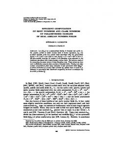
Figure 1: Power spectrum of vibrations measured in an experiment. Unavoidable manufacturing tolerances always lead to some unbalance of the rotor, which imposes a harmonic forcing of the rotor with the rotation frequency. This forcing typically leads to resonances with the first bending mode of the rotor. Furthermore, the oil lubricated journal bearings lead to self-excited oscillations of the rotor. This instability of a rigid conical mode of the rotor is known as oil whirl [7] and has been investigated since the 1920s [11, 15]. Mathematically, the nonlinear coupling of the harmonically forced rotor and the bearings leads to complicated bifurcation behavior. For example, we find torus (Neimark-Sacker) bifurcations with subsequent quasiperiodic behavior and phase locking (entrainment). In our investigation of a turbocharger model we compute tori on which quasiperiodic dynamics takes place. An important element of our study is to change coordinates to a co-rotating frame. Under certain circumstances, that is, in the case of small static loads, for example, low weight, this allows a dimension reduction so that we can compute periodic solutions instead of tori and use well-established methods with enough performance to assist in the design phase. The computationally more expensive methods for tori may be used a posteriori to verify the reduction, and to determine where the conditions for a reduction to periodic solutions are not met, for example, when the rotational speed is too low.
2
Experiments and data analysis
Several experiments were carried out at Toyota Central R&D Laboratories for a turbocharger used in vehicle engines. The turbocharger was driven by pressurized air and operated at different rotational speeds from 7500 rpm to 101000 rpm. The x- and y-deflections of the shaft were measured by eddy current sensors at both ends and in the middle of the rotor (in between the two simple journal bearings). The experimental results are shown in the frequency diagram in Figure 1. One can clearly observe the two principal vibration modes due to unbalance and oil whirl. The harmonic part has a resonance peak at about 1000 Hz and the sub-harmonic part sets in at a threshold forcing frequency of about 400 Hz. The frequency of the latter vibration is slightly less than half the forcing frequency and deviates further for higher rotational speeds. The amplitude of the sub-harmonic part decreases in the resonance region of the harmonic part. Figure 2 shows the increasingly complex behavior of the measured orbits. For small rotational speeds (250 Hz) the orbit is periodic with a small amplitude. As the driving frequency rises above 400 Hz a second frequency appears, which results in
3
EFFICIENT COMPUTATION OF QUASI-PERIODIC OSCILLATIONS
0.01
Displ y [mm]
0.1
ω=595 Hz
(b) 0.05
0.05
0
0
0
−0.005
−0.05
−0.05
−0.005
0.1
0
0.005
−0.1 −0.1
0.01
0.1
ω=998 Hz
(d)
−0.05
0
0.05
0.1
−0.1 −0.1
0.05
0.05
0
0
0
−0.05
−0.05
−0.05
−0.05
0
0.05
0.1
−0.1 −0.1
−0.05
Displ x [mm]
0
0.05
0.1
−0.1 −0.1
0
0.05
0.1
ω=1683 Hz
(f)
0.05
−0.1 −0.1
−0.05
0.1
ω=1092 Hz
(e)
ω=918 Hz
(c)
0.005
−0.01 −0.01
Displ y [mm]
0.1
ω=131 Hz
(a)
−0.05
Displ x [mm]
0
0.05
0.1
Displ x [mm]
Figure 2: Orbits of turbine dynamics (gray) overlaid with their Poincar´e sections (black) measured for different rotational speeds (note the different scale for ω = 131 Hz).
Conical mode with 464Hz (ω=998Hz) 0.01
0.005
0.005
displacement [mm]
displacement [mm]
Bending mode with 999Hz (ω=998Hz) 0.01
0
−0.005
−0.01
0
−0.005
−0.01 0
20
40 60 length [mm]
(a)
80
100
120
0
20
40 60 length [mm]
80
100
120
(b)
Figure 3: The two main vibration modes at 998 Hz; bending mode (a) and conical mode (b).
quasiperiodic dynamics on a torus. Such behavior is best analyzed by stroboscopic or Poincar´e maps: We mark the position of the turbine every time the impeller crosses the x-axis from positive to negative values. The periodic orbit of the turbine end of the shaft that we observe for low rotational speeds corresponds to a fixed point of the stroboscopic map (a). For increasing rotational speeds the Poincar´e map shows invariant circles (b)–(d) indicating the existence of invariant tori. For higher speeds the invariant circles show phase locking (e)–(f). Figure 3 shows an analysis of the mode shapes for the two kinds of vibrations. The harmonic part is mainly due to bending vibration (a), whereas the subharmonic part has a conical mode shape (b). The occurrence of the sub-harmonic has been observed a long time ago [11, 15]. This self-excited vibration is an oil whirl that is caused by the nonlinearity of the supporting oil film. In a series of papers [7, 8, 9] Muszynska clarified the occurrence and the stability of this unwanted phenomenon. In the resonance region of the first bending mode of the shaft the amplitude of the self-excited oil whirl drops; see Figure 1
4
FRANK SCHILDER ET AL. 30
Beam model
width [mm]
20
10
1
3
2
4
0
−10
−20
−30
0
20
40
60
80
100
length [mm]
(a)
(b)
Figure 4: The rotor of a turbocharger (a) and the simple beam model (b) with two disks at nodes 1 and 4 and bearings at nodes 2 and 3.
3
Finite-element rotor model
Following [15] we derive a finite beam-element model for the rotor1 . For the beam elements we consider rotating Rayleigh beams that take into account bending, rotary inertia due to bending, and gyroscopic effects, but neglect shear deformation and torsion. The rotor is split into three parts of constant diameter; see Figure 4 (b). Each element is described by lateral displacements ui and vi and inclinations φx,i and φy,i in its end-nodes z1 , . . . , z4 . We collect all displacements in the vector qi = (ui , vi , φx,i , φy,i ). The lateral displacement and the inclination along one element are interpolated from the values qi and qi+1 with the aid of the shape functions Ψ1 (σ) = 1 − 3σ 2 + 2σ 3 , � Ψ2 (σ) = σ 1 − 2σ + σ 2 ,
Ψ3 (σ) = σ 2 (3 − 2σ), Ψ4 (σ) = σ 2 (σ − 1),
on the standard element σ ∈ [0, 1]. These shape functions are solutions of normalized static deflection problems. Two rigid disk elements representing the turbine and compressor wheels are attached to the shaft in nodes 1 and 4 and their motion is completely described by the coordinates of these nodes. Using standard variational techniques [10] and setting x = (q1 , q2 , q3 , q4 ) we obtain the equation of motion ˆ L(x) = Mx ¨ + (C + ωG)x˙ + Kx = Fb (x, x) ˙ + Fg + ω 2 A(ωt)Funb (1) ˆ is a second order differential operator with symmetric mass, for the shaft. Here, L damping and stiffness matrices M , C, and K, respectively, and skew-symmetric gyroscopic matrix G. Furthermore, ω is the angular velocity of the rotor and Fg is the gravitational force. The forces exerted by the oil lubricated journal bearings in nodes 2 and 3 are given by Fb . These forces are computed from the pressure distribution in the bearings, which is modeled by the short bearing approximation to Reynolds’ equation using G¨ umbel boundary conditions; for more details see [1, 14]. The oscillating forces due to unbalance are modeled by the term ω 2 A(ωt)Funb , where Funb is a constant vector and A(ωt) is a 16 × 16 block-diagonal rotation matrix with eight 2 × 2 diagonal blocks of the form � � cos ωt − sin ωt . B(ωt) = sin ωt cos ωt 1 More details of the automobile engine turbocharger model developed by J. R¨ ubel, J. Starke, A. Kawamoto, T. Abekura and M. Inagaki, as well as experimental, simulation and bifurcation results will appear elsewhere.
EFFICIENT COMPUTATION OF QUASI-PERIODIC OSCILLATIONS −1
5
T
Note that A(ωt) = A(ωt) and kA(ωt)k2 = 1. A drawback of system (1) is that the absolute value of the time-dependent unbalance forces ω 2 A(ωt)Funb is large since this term grows quadratically with the driving frequency. As an important part of our approach, we transform equation (1) into a co-rotating frame and try to eliminate the explicit dependence on time. For the model coordinates qi = (ui , vi , φx,i , φy,i ) in the fixed frame as above, let pi be the corresponding coordinates in a frame that is rotating about the z-axis with rotational speed ω. That is, we apply the transformation � � B(ωt) 0 qi = pi , 0 B(ωt) which leads to the equation of motion T ˜ = Feb (y, y) Ly ˙ + A(ωt) Fg + ω 2 Funb ,
(2)
where y = (p1 , p2 , p3 , p4 ) is the collection of coordinates in the co-rotating frame. T The time-dependent term A(ωt) Fg is a 2π/ω-periodic forcing due to gravity. Systems (1) and (2) both are 16-dimensional second-order ordinary differential equation (ODE) with right-hand sides that explicitly depend on time. For computational purposes we transform these equations into equivalent 32-dimensional first order ODEs. The advantage of equation (2) over (1) is that for higher rotational speeds the gravitational force is small compared with the bearing and unbalance forces. This raises the question whether or not the influence of gravity can be omitted under certain circumstances. If we neglect the gravitational forcing, then Equation (2) no longer depends explicitly on time. This greatly simplifies the numerical treatment of the turbocharger model, because the dynamics on the torus can then be decomposed into two independent oscillations. One oscillation is just the forcing ωt taken modulo 2π, and the other is a periodic solution with frequency ω2 of the now autonomous Equation 2. The computation of periodic solutions is a matter of seconds to minutes, but the computation of tori requires minutes to hours or even days. The main complication is, that a torus is a two-dimensional surface, whereas a periodic solution is a one-dimensional curve. While the computation time depends only little on the dimension of the system, it increases dramatically with the dimension of the object of interest.
4
Computational performance analysis
A popular approach for the numerical investigation of response solutions is simulation, that is, solving a sequence of initial value problems for an ODE model over a range of parameters of interest. In combination with tools for classifying solutions, one can compute so-called brute-force bifurcation diagrams. This technique is usually very time consuming, even though one can easily distribute the workload by subdividing the parameter ranges. An alternative is to use more efficient numerical continuation and bifurcation methods. These techniques not only provide efficient means of computing certain types of solutions, but also allow one to detect and classify bifurcations. For the computation of equilibria and periodic solutions one can use well-established software packages, for example, AUTO [3] that provide methods for detecting pitchfork, transcritical, period-doubling, and Neimark-Sacker bifurcations. Furthermore, loci of such bifurcations can be computed in a two-parameter plane. As yet, there is no software available for the computation of invariant tori, which is currently an active area of research. We present below a recently developed method for the numerical continuation of quasiperiodic tori.
6
FRANK SCHILDER ET AL.
Solution Segments x(t +T ) 0
x(t0)
1
x(t ) 0
uN(θ)
(a)
(b)
Figure 5: Illustration of the invariance equation (3). The solution curve starting at the point x(t0 ) crosses the invariant circle again in the point x(t0 + T1 ) after one period (a). In angular coordinates on the invariant circle we have x(t0 + T1 ) = u(θ0 + 2π̺). If we identify the circles at both ends of the tube, we obtain a torus (b).
4.1
Numerical method
A vibration with two or more (but finitely many) incommensurate frequencies is a quasiperiodic solution of the ODE (2). A quasiperiodic solution never repeats and densely covers an invariant torus in phase space; see the experimental data in Figure 2. In [12] we presented a method, which we also apply here, for the computation of quasiperiodic solutions with two incommensurate frequencies; see also [5, 13]. The basic idea of this method is to compute an invariant circle of the period-2π/ω1 stroboscopic map, which is the intersection of the torus with the plane t = 0. Here, ω1 = ω is the forcing frequency and we interpret time as an angular variable modulo the forcing period. By construction, the invariant circle has rotation number ̺ = ω2 /ω1 , where ω2 is the additional response frequency of the occurring vibration. An invariant circle with rotation number ̺ is a solution of the so-called invariance equation u(θ + 2π̺) = g(u(θ)),
(3)
where u is a 2π-periodic function and g is the period-2π/ω1 stroboscopic map of (2). We approximate the invariant circle u with a Fourier polynomial of the form uN (θ) = c1 +
N X
c2k sin kθ + c2k+1 cos kθ
(4)
k=1
and compute the real coefficient vectors c1 , . . . , c2N +1 by collocation. The stroboscopic map g is computed with the second-order fully implicit midpoint rule as the solution of a two-point boundary value problem; see [12] and Figure 5 for more details. We construct seed solutions for our subsequent continuations of tori with the method of homotopy. To this end, we introduce an artificial parameter λ ∈ [0, 1] as an amplitude of the gravitational forcing: T ˜ = Feb (y, y) Ly ˙ + λA(ωt) Fg + ω 2 Funb .
(5)
We refer to the case λ = 0 as the zero-gravity system and the case λ = 1 as the Earth-gravity system. The principle of homotopy is to compute a torus for λ = 0 and try to follow this torus as λ is slowly increased up to λ = 1. For λ = 0 equation (5) becomes autonomous and we can construct an invariant torus directly from a Fourier approximation (4) of a periodic solution with frequency ω2 . This can be seen from the definition of the period-2π/ω1 stroboscopic map of the T2 = 2π/ω2 -periodic
7
EFFICIENT COMPUTATION OF QUASI-PERIODIC OSCILLATIONS 1150
0.4
0.4
0.3
0.3
1000 950
1
2
3
4
900 850
Displ y [mm]
1050
Displ y [mm]
Driving Frequency [Hz]
1100
0.2 0.1
2
4 3
0
1
0.2 0.1
4
2
3
0
1
800 −0.1
−0.1
750 700 0
0.01 0.02 0.03 0.04 0.05 0.06 0.07 0.08
−0.2 −0.3
−0.2
−0.1
Bearing Clearance [mm]
0
0.1
Displ x [mm]
(a)
(b)
0.2
0.3
−0.2 −0.3
−0.2
−0.1
0
0.1
0.2
0.3
Displ x [mm]
(c)
Figure 6: Positions of the seed solutions (label ×) and corresponding earth-gravity tori (label ◦) in the (cr , ω) plane (a). The invariant circles for Earth gravity (b) and the corresponding periodic solutions for zero gravity (c) for the starting positions along the row near ω ≈ 894 Hz. The tori at the labeled positions are shown in Figure 7.
solution x(t) = uN (ω2 t) = uN (θ), where uN is our Fourier polynomial of order N with the scaling ω2 t = θ. Then, x(t + T1 ) = g(x(t)) = g(uN (θ)) by definition, and we also have x (t + T1 ) = x
�
2π θ + ω2 ω1
�
=x
�
� �� ω2 1 θ + 2π = uN (θ + 2π̺) . ω2 ω1
Finally, a solution segment connecting a starting point x(t0 ) with the endpoint x(t0 + T1 ) is given by uN (θ), where (θ − t0 /ω2 ) ∈ [0, 2π̺]; see Figure 5. For the system under consideration it turns out that the zero-gravity tori are such accurate approximations to the Earth-gravity tori that the latter can be computed in just one homotopy step; compare panels (b) and (c) of Figure 6 where we computed a series of tori for varying radial bearing clearance cr and driving frequency ω. The fact that the zero-gravity tori are almost identical to the Earth-gravity tori is a first indication that the negligence of gravitation is a valid and powerful simplification of the model equation. Recall that the reason for performing such a simplification whenever feasible is the fact that the numerical analysis of invariant tori (for λ = 1) is a much harder problem than the analysis of periodic solutions (for λ = 0). Furthermore, the dependence of periodic solutions on system parameters can be studied by changing the parameters individually. This is no longer true for quasiperiodic tori, because a quasiperiodic vibration with two incommensurate frequencies can be changed into a phase-locked state by arbitrarily small changes in any parameter. Therefore, one simultaneously needs to adjust a second free parameter to ‘follow’ solutions with a fixed frequency ratio. Thus, paths of quasiperiodic tori are curves in a two-parameter plane: for example, note the slight shift in some of the positions of Earth-gravity tori in Figure 6 (a) with respect to the seed solutions. The union of these curves covers a set of large measure [6]. In other words, there is a non-zero probability to observe quasiperiodic behavior in physical systems. We emphasize at this point that, according to the above construction, the computation of periodic solutions for λ = 0 is equivalent to a computation of invariant tori for λ = 0. Our claim is, that these tori are good approximations to the tori for λ = 1 for certain parameters. Our method allows to identify such parameter regions where neglecting gravity is a sound assumption. In these regions one can obtain the response behavior of the turbocharger model by studying the periodic solutions of the autonomous ODE (5) with λ = 0.
8
4.2
FRANK SCHILDER ET AL.
Computational results
We focus here on computations that demonstrate the performance of our numerical technique and help us test the validity of the zero-gravity assumption. We sweep a parameter plane with a large number of paths of Earth-gravity quasiperiodic tori in the (cr , ω)-plane to obtain a picture as complete as possible. For comparison and for verifying the zero-gravity approximation we perform the respective computations of periodic solutions. Towards the end of this section we give some physical interpretation of the results. All our computations were performed on equation (5) in co-rotating coordinates. First, we compute a Fourier approximation of the periodic solution of the zerogravity system for ω = 1000 Hz and cr = 0.02 mm. This is done by simulation and a subsequent Fourier transformation with N = 15 Fourier modes in (4). We then perform a continuation of the periodic solution with respect to the forcing frequency and select the solutions that are shown as the column of crosses for cr = 0.02 in Figure 6 (a) in the frequency window ω ∈ [700 Hz, 1200 Hz], which is a principal range of operation for the turbocharger. In a second run, we compute the start solutions marked by the three rows of crosses for frequencies ω = 797 Hz, 894 Hz and 1037 Hz in the range cr ∈ [0.01 mm, 0.08 mm], which represents the design margin of the device. As explained in the previous section, we construct initial approximations of tori in the Earth-gravity system from these periodic solutions. We computed these tori with N = 15 Fourier modes and M = 100 Gauß collocation points and keep this mesh size fixed for all subsequent computations. In the homotopy step we keep the radial bearing clearance cr fixed and take the forcing frequency as a secondary free parameter. The obtained starting positions of tori are marked with circles in Figure 6 (a). The idea is that with this distribution of starting solutions the paths of tori cover the (cr , ω)-plane densely enough to allow meaningful conclusions. Note that the starting positions virtually coincide with the seed positions. The differences in the forcing frequencies mean that tori with a certain rotation number are observed for slightly different rotational speeds in the two systems. In other words, the response frequencies differ somewhat. A first comparison of the two types of solutions is given in panels (b) and (c) of Figure 6. Both graphs illustrate the change of the invariant circle in the stroboscopic map as the bearing clearance is increased and the forcing frequency is kept (approximately) constant. The two sets of circles are clearly very similar. The full tori for the starting positions labeled 1 to 4 are shown in Figure 7 together with a plot of the displacements at node 1. Even though our finite beam-element model is rather coarse, the numerical results resemble the qualitative features of the measured orbits; compare Figure 7 (b) with Figure 2 (c). Note that the Poincar´e sections are defined differently in these figures. A comparison of the two sets of resulting two-parameter paths is shown in Figure 8 with arcs of tori with fixed rotation number in panel (a) and arcs of periodic solutions with fixed frequency ratio in panel (b). The grey scale of each path indicates its associated rotation number. The second response frequency ω2 is the product of this rotation number with the driving frequency shown on the vertical axis. These curves match very well: Only in a band around 900 Hz there are some visible differences, but they are small. At a first glance we observe that in the region covered ω2 is approximately half the driving frequency, in accordance with the experimental data; see Figure 1. If we keep the bearing clearance fixed at 0.02 mm, as used in the current design of the turbocharger, and increase the driving frequency, then the rotation number increases initially, stays almost constant for ω ∈ [830 Hz, 970 Hz] and then starts to decrease. This behavior reflects the ‘bending’ of the oil-whirl response frequency away from the straight line ω2 = 0.5ω in Figure 1.
9
EFFICIENT COMPUTATION OF QUASI-PERIODIC OSCILLATIONS
0.3
(a)
0.2
0
Displ y1 [mm]
Displ x2 [mm]
0.05
−0.05
l Disp
0.2
x 1 [m m]
−0.4
0.3
0.2
0.1
0
−0.1
−0.4
−0.2
−0.2
Displ y 1 [mm]
0
0.2
0.4
0
0.2
0.4
0
0.2
0.4
0
0.2
0.4
Displ x1 [mm]
0.3
(b)
0.2
0
Displ y1 [mm]
Displ x2 [mm]
−0.1 −0.2
0
−0.05
Disp
0.2
0.1 0 −0.1
l x1
−0.2
0
[mm
−0.2
]
−0.4
0.3
0.2
0.1
0
−0.1
−0.4
−0.2
−0.2
Displ y 1 [mm]
0.05
Displ x1 [mm]
0.3
(c)
0.2
0
Displ y1 [mm]
Displ x2 [mm]
0
−0.2
0.05
−0.05
Disp
0.2
0.1 0 −0.1
l x1
−0.2
0
[mm
−0.2
]
−0.4
0.3
0.2
0.1
0
−0.1
−0.4
−0.2
−0.2
Displ y 1 [mm]
0.05
Displ x1 [mm]
0.3
(d)
0.2
0
Displ y1 [mm]
Displ x2 [mm]
0.1
−0.05
l x1
Disp
0.2
0.1 0 −0.1 −0.2
0
[mm
−0.2
]
−0.4
0.3
0.2
0.1
0
−0.1
Displ y 1 [mm]
−0.2
−0.4
−0.2
Displ x1 [mm]
Figure 7: The left-hand column of (a)–(d) shows starting tori with labels 1, 2, 3 and 4, respectively, along the row ω = 894 Hz in Figure 6 (a). The corresponding x- and y-displacements at the first FEM-node are shown in the right-hand column. The dark closed curve is the invariant circle of the period-2π/ω1 stroboscopic map.
10
FRANK SCHILDER ET AL.
1150
(a)
0.541
1100 0.536
1000 0.530 950 0.524
900 850
Rotation number
Driving Frequency [Hz]
1050
0.519
800 0.513 750 700 0
0.01
0.02
0.03
0.04
0.05
0.06
0.07
0.08
1150
(b)
0.541
Driving Frequency [Hz]
1050
0.536
1000 0.530 950 0.524
900 850
0.519
800
Forcing−response frequency ratio
1100
0.513 750 700 0
0.01
0.02
0.03
0.04
0.05
0.06
0.07
0.08
Bearing Clearance [mm]
Figure 8: Curves of quasiperiodic tori with fixed rotation number of the Earthgravity system (a), curves of periodic solutions with fixed frequency ratio of the zero-gravity system (b). The grey scale of the curves indicate their associated rotation number or frequency ratio. The dashed curves are loci of Neimark-Sacker bifurcations (a) and Hopf bifurcations (b), respectively. The diagram gives an overview of the second response frequency as a function of the bearing clearance and the forcing frequency. It also shows that the second frequency is suppressed for bearing clearances smaller than 0.01 mm.
EFFICIENT COMPUTATION OF QUASI-PERIODIC OSCILLATIONS
11
Figure 8 also shows two bifurcation curves (dashed), namely, a locus of NeimarkSacker bifurcations (a) and a locus of Hopf bifurcations (b). Again, these curves match very well. For small bearing clearance, to the left of the Neimark-Sacker curve, the response is periodic and has the same frequency as the forcing; this corresponds to an equilibrium solution for the zero-gravity system. If we cross this curve from left to right the quasiperiodic response considered above is born and its amplitude grows rapidly as the bearing clearance is further increased; see Figures 6 (b) and 7. This behavior is also accurately captured in the zero-gravity system as is illustrated with panels (b) and (c) of Figure 6, where periodic solutions are compared with invariant circles of tori along the line ω = 894 Hz. These results indicate that for the range of forcing frequencies considered here a reduction of the bearing clearance could dramatically reduce the amplitude of the quasiperiodic vibration or even suppress the second frequency completely. Figure 8 (a) shows a total of 51 curves of tori and along each curve we computed 200 tori (this is the reason why some curves end in the middle of the figure). The computation of the tori took approximately four weeks on an Intel Xeon CPU 2.66GHz, that is, the average time to compute one torus is about four minutes. The computation of the corresponding curves of periodic solutions in panel (b) with the same number of solutions along each curve was completed within 24 hours, that is, the computation of one periodic solution takes about nine seconds. Hence, the transition to the zero-gravity system results in a large gain in performance, possibly at the expense of some accuracy. However, as our computations show, the qualitative behavior of the two systems virtually coincides, and one might ask whether the introduced approximation error is at all significant. Our results clearly suggest that one should perform an analysis of periodic solutions for the zero-gravity system and look at the Earth-gravity system only when absolutely necessary.
5
Conclusions
In this paper we demonstrated the efficient computation of invariant tori for a simple finite beam-element turbocharger model. Our investigation verified that one can neglect gravitational forces for higher rotational speeds. We showed that this leads to a dramatic reduction of computational effort if the model is formulated in co-rotating coordinates. The reason is that invariant tori of the Earth-gravity system are then well approximated by tori constructed from periodic solutions of the zero-gravity system. The computation of periodic solutions is a much simpler task and there are well-established and highly efficient methods at hand that could be applied to substantially more detailed models of a turbocharger, or other machinery with fast rotating parts. If gravity or other static loads cannot be considered a small perturbation, then one must compute invariant tori in the Earth-gravity system. Such a computation is far more challenging and there are only few methods available. The recently developed method [12] used here works well for moderately large systems and shows a typical trade-off: the computation of tori requires more memory than long-term simulation since all mesh points and a large sparse matrix need to be stored simultaneously, but, on the other hand, it is faster, more accurate and provides more detailed information about the dynamics. Furthermore, it allows to compute unstable tori and, thus, the direct analysis of hysteresis effects. The techniques used here for the turbocharger model are also applicable more widely. In particular, for other systems with fast rotating parts it may be possible to neglect the influence of gravity and obtain the powerful reduction as discussed in this paper. The value of invariant torus computation is that it allows one to verify the validity of the model reduction. In this case, a bifurcation diagram showing the qualitative behavior of the response solutions can be obtained with the computation of periodic solutions alone.
12
FRANK SCHILDER ET AL.
Acknowledgements This work was supported by EPSRC grant GR/R72020/01, Toyota CRDL and the University of Heidelberg.
References [1] D. Childs. Turbomachinery Rotordynamics. Wiley, 1993. [2] S. H. Crandall. Rotordynamics. In W. et al. Kliemann, editor, Nonlinear Dynamics and Stochastic Mechanics. Dedicated to Prof. S. T. Ariaratnam on the occasion of his sixtieth birthday, CRC Mathematical Modelling Series, pages 3–44. CRC Press, 1995. [3] E.J. Doedel, A.R. Champneys, T.F. Fairgrieve, Yu.A. Kuznetsov, B. Sandstede, and X. Wang. Auto97: Continuation and bifurcation software for ordinary differential equations (with HomCont). Technical report, Concordia University, 1997. [4] R. Gasch, R. Nordmann, and H. Pf¨ utzner. Rotordynamik. Springer, 2nd edition, 2002. [5] T. Ge and A. Y. T. Leung. Construction of invariant torus using Toeplitz Jacobian matrices/fast Fourier transform approach. Nonlinear Dynam., 15(3):283– 305, 1998. [6] James A. Glazier and Albert Libchaber. Quasi-periodicity and dynamical systems: an experimentalist’s view. IEEE Trans. Circuits and Systems, 35(7):790– 809, 1988. [7] A. Muszynska. Whirl and whip – rotor/bearing stability problems. Journal of Sound and Vibration, 110(3):443–462, 1986. [8] A. Muszynska. Tracking the mystery of oil whirl. Sound and Vibration, pages 8–11, February 1987. [9] A. Muszynska. Stability of whirl and whip in rotor/bearing systems. Journal of Sound and Vibration, 127(1):49–64, 1988. [10] H. D. Nelson and J. M. McVaugh. The dynamics of rotor-bearing systems using finite elements. Transactions of the ASME, Journal of Engineering for Industry, pages 593–600, May 1976. [11] B. L. Newkirk and H. D. Taylor. Shaft whirling due to oil action in journal bearings. Gen. Electr. Rev., 28(7):559–568, 1925. [12] Frank Schilder and Bruce B. Peckham. Computing Arnol′d tongue scenarios. Technical Report BCANM.280, University of Bristol, 2006. [13] Frank Schilder, Stephan Schreiber, Werner Vogt, and Hinke M. Osinga. Fourier methods for quasi-periodic oscillations. Int. J. Numer. Meth. Engng., 2006. to appear, early view: http://www3.interscience.wiley.com/cgibin/jissue/108567238. [14] J. M. Vance. Rotordynamics of Turbomachinery. Wiley, 1988. [15] T. Yamamoto and Y. Ishida. Linear and Nonlinear Rotordynamics. Wiley, 2001.