Abstract. The concept of safe region has been used to reduce the com- putation and communication cost for the continuous monitoring of k nearest neighbor ...
Efficient Construction of Safe Regions for Moving kNN Queries Over Dynamic Datasets Mahady Hasan, Muhammad Aamir Cheema, Xuemin Lin, Ying Zhang The University of New South Wales, Australia {mahadyh,macheema,lxue,yingz}@cse.unsw.edu.au
Abstract. The concept of safe region has been used to reduce the computation and communication cost for the continuous monitoring of k nearest neighbor (kNN) queries. A safe region is an area such that as long as a query remains in it, the set of its kNNs does not change. In this paper, we present an efficient technique to construct the safe region by using cheap RangeNN queries. We also extend our approach for dynamic datasets (the objects may appear or disappear from the dataset). Our proposed algorithm outperforms existing algorithms and scales better with the increase in k.
1
Introduction
With the availability of inexpensive mobile devices, position locators and cheap wireless networks, location based services are gaining increasing popularity. The continuous monitoring of k nearest neighbor (kNN) queries [1–4] has been widely studied in recent past. In this paper, we study the problem of moving kNN queries where the query is constantly moving and the objects do not move. Consider the example of a car driver who is interested in five nearest available car parking spaces while driving in a city. Another example is a person looking for the nearest restaurants while walking in a street. A classical example of the safe region is Voronoi Diagram (VD) [5]. In a VD, each object of the dataset lies within a cell called its voronoi cell. The voronoi cell of an object has a property that any point that lies in it is always closer to that object than any other object in the dataset. For a kNN query, a k order VD can be constructed and k order voronoi cells can be treated as safe regions. The VD based solution has the following major limitations: 1) The VD cannot be precomputed and indexed if the value of k is not known in advance. 2) The VD cannot deal efficiently with update of objects in the underlying dataset. Our contributions in this paper include: 1) we devise an efficient safe region construction approach that requires cheap RangeNN 1 queries; 2) our proposed approach is extended to efficiently update the safe regions of queries for dynamic datasets where the objects may appear or disappear and 3) extensive experiment results show more than an order of magnitude improvement. 1
RangeNN query is to find the nearest object of q from the objects that lie within a given distance from a point p.
2
Background Information
Continuous k Nearest Neighbor Query. Given a set of objects, a moving query point q , and a positive integer k , the continuous kNN query is to continuously report k closest objects to q at each time stamp. Definitions and Notations. A perpendicular bisector Bn:o between two points n and o divides the space into two half-spaces. Let Hn:o be the half-space containing n and Ho:n be the half-space containing o. Every point q in Hn:o is always closer to n than it is to o (i.e; dist(q, n) < dist(q, o)). Figure 1 shows a bisector Bn:o2 between two points n and o2 and the two half-spaces are also shown. Safe Region S is a region such that as long as a kNN query q remains in it, the set of its kNNs does not change. If a client (that issued query q) is aware of its safe region, it does not need to contact the server to update its set of kNNs as long as q resides in the safe region. This saves the communication cost as well as computation cost. Now, we formally define the safe region. Let N = {n1 , · · · , nk } be the set of kNNs of a query q. The intersection of all half-spaces Hni :oj for every ni ∈ N and every oj ∈ O − N defines a region such that as long as the query resides in it, the set of its kNNs N is unchanged. Proof. We prove this by contradiction. Assume that q resides in its safe region and oj ∈ O − N is an object such that dist(q, oj ) < dist(q, ni ) for any ni ∈ N . Since safe region is the intersection of all half-spaces Hni :oj , a query q that resides in it satisfies dist(q, ni ) < dist(q, oj ) which contradicts the assumption. ⊓ ⊔ Figure 1 shows an example of the safe region for a NN query. The bisectors between the nearest neighbor n and the objects o1 to o4 are drawn and the shaded area is the safe region. Figure 2 shows an example of the safe region for a 2NN query where the two NNs are n1 and n2 . The bisectors between the NNs and the objects o1 to o3 are drawn. For clarity, the bisectors between n1 and the objects are shown in solid lines and the bisectors between n2 and the objects are shown in broken lines. The shaded area is the safe region. Note that not all the bisectors contribute in defining the safe region. A bisector Bni :oj that forms an edge of the safe region is called a representative bisector (the bisector Bn:o2 in Fig. 1). The object oj that is associated with the representative bisector is called an influence object (o2 in Fig. 1). Notation Bx:q Hx:q Hq:x dist(x, y) v ≺ Bni :oj ∩ Bnx :oy ≻
Definition a perpendicular bisector between point x and q a half-space defined by Bx:q containing the point x a half-space defined by Bx:q containing the point q the distance between two points x and y a vertex v formed by the intersection of the two bisectors Table 1. Notations
A vertex is the intersection of two bisectors Bni :oj and Bnx :oy . A confirmed vertex is the vertex of the safe region (i.e., it is an intersection of two representative bisectors). Vertex v in Fig. 1 is a confirmed vertex whereas the vertex v ′ is not a confirmed vertex. Please note that a confirmed vertex lies at the boundary of the safe region. Table 1 defines the notations used throughout this paper.
The most related work to our technique is proposed in [6]. The authors propose construction of the safe region by using time parameterized kNN queries [7]. Due to space limitations, we omit the details.
3
Technique
Before we present our algorithm, we present observations that can be used to confirm a vertex. First, we present the observation for k = 1 and then we extend it for arbitrary value of k. Bn:o
4
o4
o1
o1 v'
n
v
q
Bn:o
o2
o1 n1
2
q n2
o3
o3 Hn:o
2
Ho2:n
Fig. 1. Safe region for a NN query
n1q n2
o2
o3
o2 v
o4
Fig. 2. Safe region for a 2NN query
Fig. 3. Illustration of Observation 2
Observation 1 : Let n be the NN of a query q and v be a vertex. The vertex v can be confirmed if no object lies in the circle of radius R centered at v where R = dist(v, n). Proof. Assume that the circle does not contain any object and o4 (as shown in Fig. 1) is any object that lies outside the circle. If the vertex v does not lie in the safe region then there must be a half-space Ho4 :n that contains v. Any point p that lies in the half-space Ho4 :n satisfies dist(p, o4 ) < dist(p, n). However, for vertex v, dist(v, o4 ) > dist(v, n). Hence there is no such half-space Ho4 :n that contains v. So the vertex v lies in the safe region. ⊓ ⊔ Observation 2 : Let N = {n1 , · · · , nk } be the set of kNNs of query q and v be any vertex. The vertex v can be confirmed if no object o ∈ O − N lies in the circle centered at v with radius R = maxdist(v, N ) where maxdist(v, N ) is max(dist(v, ni )) for every ni ∈ N . Proof. Assume that the circle does not contain any object and o4 is any object that lies outside the circle (as shown in Fig. 3). The vertex v satisfies dist(v, ni ) < dist(v, o4 ) for every ni ∈ N , hence v lies in every Hni :o4 . For this reason, the vertex v lies in the safe region. ⊓ ⊔ Algorithm 1 presents the construction of the safe region for a kNN query. The algorithm maintains a set of vertices V (initialized to four vertices of the universal data space). First, the set N containing kNNs of the query q is computed by using BFS [8]. Then, the algorithm randomly selects an unconfirmed vertex v from V and checks whether it can be confirmed or not by using Observation 2. More specifically, the algorithm checks whether there is any object in the circle
Algorithm 1 Construct Safe Region (q) 1: V = {Vertices of the data space} 2: compute kNNs of q and store in N 3: while there is an unconfirmed vertex in V do 4: select any unconfirmed vertex v 5: R = maxdist(v, N ) 6: o = RangeNN(q, v, R)/* Algorithm 2 */ 7: if o = N U LL then 8: confirm v 9: else 10: update V using bisectors between o and each ni ∈ N
of range R = maxdist(v, N ) centered at v. If there is no object in the circle, the algorithm marks the vertex as confirmed (line 8). If there are more than one objects in the circle, the algorithm selects the nearest object o to the query q (line 6). The safe region is updated by considering the bisectors between kNNs of q and the object o (line 10). For a given bisector Bni :o , the safe region is updated by removing the vertices from V that lie in Ho:ni and adding the intersection points of Bni :o and the safe region. The algorithm stops when all the vertices are confirmed. To show the correctness of the algorithm, we need to show that the algorithm finds all the vertices of the safe region and does not include any unconfirmed vertex. The proof of correctness is similar to Lemma 3.1 in [6] and is omitted. Algorithm 2 RangeNN(q, v, R) Output: Returns the nearest neighbor of q from the objects that lie within distance R from v 1: Initialize a min-heap H with root entry of the tree 2: while H is not empty do 3: deheap an entry e 4: if e is an intermediate or leaf node then 5: for each of its children c do 6: if mindist(c, v) < R then 7: insert c into H with key mindist(c, q) 8: else if e is an object and e is not one of the kNNs of q then 9: return e 10: return φ
Algorithm 2 presents the implementation of RangeNN query. This operation can be regarded as finding the nearest object o of q from the objects lying within the range R of a vertex v. Hence, we call it RangeNN query. Example 1. Figure 4 illustrates our algorithm for a 2NN query where n1 and n2 are the NNs of q. Initial safe region is the data space bounded by four vertices v1 to v4 . First, a RangeNN 2 query is issued on vertex v1 with range R = dist(v1 , n1 ) which returns the object o3 . Then, the bisectors between o3 and the NNs are 2
Note that RangeNN query does not access all the objects within the range. It uses BFS and stops when the NN is found. So the object o4 is not accessed in the example.
v3
v4
v3
v8
v6
o1 n1
v4
q
q
o2
n2
v9
n1 n2
o3
v2
Fig. 4. RangeNN query from v1
v1
v
v5
o4
o4
o2
n1q n2
o2
o3
o3
v1
o1
o1
v7
v2
Fig. 5. The safe region after visiting o3
Fig. 6. Safe Region and impact Region
drawn. In Fig. 5, the bisector between o3 and n1 is shown in solid line and the bisector between o3 and n2 is shown in broken line. These bisectors update the set of vertices V and the new safe region (the shaded area) now contains vertices v3 , v5 , v9 and v8 . Then, a RangeNN query is issued on vertex v9 with range dist(v9 , n1 ) and it is marked confirmed because no object is found within the range. The algorithm continues in this way until all the vertices are confirmed. The final safe region is shown in Fig. 6 (light shaded area). Extension for Dynamic Datasets. First, we define impact region. The impact region is an area such that as long as a query remains in its safe region and no object appears or disappears from the impact region, the safe region of the query is unchanged. It is easy to prove that the impact region consists of circles around vertices with radius set to their corresponding nearest neighbors. In Fig. 6, the impact region is shown shaded (both dark and light). Below, we formally define the impact region. Let V be a set of vertices of a safe region. Let Circv be a circle centered at a vertex v ≺ Bni :oj ∩ Bnx :oy ≻ with radius Rv = dist(v, ni ). The impact region is the area covered by all circles Circvi for each vi ∈ V . We use a grid-based structure and mark all the cells that overlap with the impact region. The results of a query are affected only if an object appears in (or disappears from) these marked cells. For such queries, we compute the safe regions again.
4
Experimental Study and Remarks
We compare our algorithm with LBSQ [6]. Other algorithms for moving kNN queries either assume known query trajectory path [7, 4] or assume that clients have sufficient computation resources to maintain kNNs from given (k + x) or more NNs [9–11]. We use real dataset (http://www.census.gov/geo/www/tiger/) that contains 128,700 unique data points in a data space of 350km×350km. We continuously monitor 500 moving queries created by the spatio-temporal data generator [12].
10000
12 LBSQ RSR 10
90K 60K
8 6 LBSQ=0.3
4
RSR=0.07
178
3
10
30
100
k values
Fig. 7. Total RangeNN / TPkNN queries
38.5
1
3
10
30
100
k values
Fig. 8. Average cost of RangeNN / TPkNN query
9.9
5.9 2.1
0 0 1
1474
100
10
2
30K
LBSQ RSR
1000 Time in sec
RSR LBSQ
120K Time in ms
# of RangeNN/TPkNN queries
150K
37 11
4.9
2.6
1 1
3
10
30
100
k values
Fig. 9. The computation time for different k
Figure 7 shows that the number of RangeNN queries is slightly higher than the number of TPkNN queries, but the average cost of a RangeNN query is significantly lower than that of a TPkNN query (Fig. 8). Figures 9 studies the effect of k on the computation times of both algorithms (shown in log scale). Our algorithm not only outperforms LBSQ but also scales better. We also observed that the number of nodes accessed by our algorithm is lower than that of LBSQ but we do not include the figure due to page limitation. Previous algorithm uses TPkNN queries to compute the safe region of a kNN query. In this paper, we present an efficient algorithm to construct the safe region by using much cheaper RangeNN queries. Experiment results show an order of magnitude improvement.
References 1. Mouratidis, K., Hadjieleftheriou, M., Papadias, D.: Conceptual partitioning: An efficient method for continuous nearest neighbor monitoring. In: SIGMOD Conference. (2005) 634–645 2. Yu, X., Pu, K.Q., Koudas, N.: Monitoring k-nearest neighbor queries over moving objects. In: ICDE. (2005) 631–642 3. Xiong, X., Mokbel, M.F., Aref, W.G.: Sea-cnn: Scalable processing of continuous k-nearest neighbor queries in spatio-temporal databases. In: ICDE. (2005) 643–654 4. Tao, Y., Papadias, D., Shen, Q.: Continuous nearest neighbor search. In: VLDB. (2002) 287–298 5. Okabe, A., Boots, B., Sugihara, K.: Spatial tessellations: concepts and applications of Voronoi diagrams. John Wiley and Sons Inc. (1992) 6. Zhang, J., Zhu, M., Papadias, D., Tao, Y., Lee, D.L.: Location-based spatial queries. In: SIGMOD Conference. (2003) 443–454 7. Tao, Y., Papadias, D.: Time-parameterized queries in spatio-temporal databases. In: SIGMOD Conference. (2002) 334–345 8. Hjaltason, G.R., Samet, H.: Ranking in spatial databases. In: SSD. (1995) 83–95 9. Kulik, L., Tanin, E.: Incremental rank updates for moving query points. In: GIScience. (2006) 251–268 10. Song, Z., Roussopoulos, N.: K-nearest neighbor search for moving query point. In: SSTD. (2001) 79–96 11. Nutanong, S., Zhang, R., Tanin, E., Kulik, L.: The v*-diagram: a query-dependent approach to moving knn queries. PVLDB 1(1) (2008) 1095–1106 12. Brinkhoff, T.: A framework for generating network-based moving objects. GeoInformatica 6(2) (2002) 153–180