ful hardware and software model checking techniques. Efficient algorithms ...... rank. Let [E 0] denote the HNF of C. If CX = D has no integral solution, then Eâ1D.
Efficient Craig Interpolation for Linear Diophantine (Dis)Equations and Linear Modular Equations ? Himanshu Jain1 , Edmund Clarke1 , and Orna Grumberg2 1
2
School of Computer Science, Carnegie Mellon University Department of Computer Science, Technion - Israel Institute of Technology
Abstract. The use of Craig interpolants has enabled the development of powerful hardware and software model checking techniques. Efficient algorithms are known for computing interpolants in rational and real linear arithmetic. We focus on subsets of integer linear arithmetic. Our main results are polynomial time algorithms for obtaining interpolants for conjunctions of linear diophantine equations, linear modular equations (linear congruences), and linear diophantine disequations. We show the utility of the proposed interpolation algorithms for discovering modular/divisibility predicates in a counterexample guided abstraction refinement (CEGAR) framework. This has enabled verification of simple programs that cannot be checked using existing CEGAR based model checkers.
1
Introduction
The use of Craig interpolation [8] has led to powerful hardware [14] and software [9] model checking techniques. In [14] the idea of interpolation is used for obtaining overapproximations of the reachable set of states without using the costly image computation (existential quantification) operations. In [9, 11] interpolants are used for finding the right set of predicates in order to rule out spurious counterexamples. An interpolating theorem prover performs the task of finding the interpolants. Such provers are available for various theories such as propositional logic, rational and real linear arithmetic, and equality with uninterpreted functions [15, 21, 12, 11, 19, 13, 6]. Efficient algorithms are known for computing interpolants in rational and real linear arithmetic [15, 19, 6]. Linear arithmetic formulas where all variables are constrained to be integers are said to be formulas in (pure) integer linear arithmetic or LA(Z), where Z is the set of integers. There are no known efficient algorithms for computing interpolants for formulas in LA(Z). This is expected because checking the satisfiability of conjunctions of atomic formulas in LA(Z) is itself NP-hard. We show that for various subsets of LA(Z) one can compute interpolants efficiently. Informally, a linear equation where all variables are integer variables is said to be a linear diophantine equation (LDE). A linear modular equation (LME) or a linear congruence over integer variables is a type of linear equation that expresses divisibility relationships. A system of LDEs (LMEs) denotes conjunctions of LDEs (LMEs). Both LDEs and LMEs arise naturally in program verification when modeling assignments and conditional statements as logical formulas. These subsets of LA(Z) are also known ?
This research was sponsored by the Gigascale Systems Research Center (GSRC), the Semiconductor Research Corporation (SRC), the Office of Naval Research (ONR), the Naval Research Laboratory (NRL), the Army Research Office (ARO), and the General Motors Lab at CMU.
to be tractable, that is, polynomial time algorithms are known for deciding systems of LDEs and LMEs. We study the interpolation problem for LDEs and LMEs. Given formulas F, G such that F ∧ G is unsatisfiable, an interpolant for the pair (F, G) is a formula I(F, G) with the following properties: 1) F implies I(F, G), 2) I(F, G) ∧ G is unsatisfiable, and 3) I(F, G) refers only to the common variables of F and G. This paper presents the following new results. • F, G denote a system of LDEs: We show that I(F, G) can be obtained in polynomial time by using a proof of unsatisfiability of F ∧ G. The interpolant can be either a LDE or a LME. This is because in some cases there is no I(F, G) that is a LDE. In these cases, however, there is always an I(F, G) in the form of a LME. (Sec. 3) • F, G denote a system of LMEs: We obtain I(F, G) in polynomial time by using a proof of unsatisfiability of F ∧ G. We can ensure that I(F, G) is a LME. (Sec. 4) • Let S denote an unsatisfiable system of LDEs. The proof of unsatisfiability of S can be obtained in polynomial time by using the Hermite Normal Form of S (represented in matrix form) [20]. A system of LMEs R can be reduced to an equisatisfiable system of LDEs R0 . The proof of unsatisfiability for R is easily obtained from the proof of unsatisfiability of R0 . (Sec. 5) • Let S denote a system of LDEs. We show that if S has an integral solution, then every LDE that is implied by S, can be obtained by a linear combination of equations in S. We show that S is convex [17], that is, if S implies a disjunction of LDEs, then it implies one of the equations in the disjunction. In contrast, conjunctions of atomic formulas in LA(Z) are not convex due to inequalities [17]. These results help in efficiently dealing with linear diophantine disequations (LDDs). (Sec. 6) • Let S = S1 ∧ S2 , where S1 is a system of LDEs, while S2 is a system of LDDs. We say that S is a system of LDEs+LDDs. We show that S has no integral solution if and only if S1 ∧S2 has no rational solution or S1 has no integral solution. This gives a polynomial time decision procedure for checking if S has an integral solution. If S has no integral solution, then the proof of unsatisfiability of S can be obtained in polynomial time. (Sec. 6) • F, G denote a system of LDEs+LDDs: We show I(F, G) can be obtained in polynomial time. The interpolant can be a LDE, a LDD, or a LME. (Sec. 6) • We show the utility of our interpolation algorithms in counterexample guided abstraction refinement (CEGAR) based verification [7]. Our interpolation algorithm is effective at discovering modular/divisibility predicates, such as 3x + y + 2z ≡ 1 (mod 4), from spurious counterexamples. This has allowed us to verify programs that cannot be verified by existing CEGAR based model checkers. Polynomial time algorithms are known for solving (deciding) a system of LDEs [20, 5] and LMEs (by reduction to LDEs) over integers. We do not give any new algorithms for solving a system of LDEs or LMEs. Instead we focus on obtaining proofs of unsatisfiability and interpolants for systems of LDEs, LMEs, LDEs+LDDs. We only consider conjunctions of LDEs, LMEs, LDEs+LDDs. Interpolants for any (unsatisfiable) Boolean combinations of LDEs can also be obtained by calling the interpolation algorithm for conjunctions of LDEs+LDDs multiple times in a satisfiability modulo theory
(SMT) framework [6]. However, computing interpolants for Boolean combinations of LMEs is difficult. This is due to linear modular disequations (LMDs). We can show that even the decision problem for conjunctions of LMDs is NP-hard. The extended version of the paper [10] contains all proofs. Related Work. It is known that Presburger arithmetic (PA) augmented with modulus operator (divisibility predicates) allows quantifier elimination. Kapur et al. [12] show that a recursively enumerable theory allows quantifier-free interpolants if and only if it allows quantifier elimination. The systems of LDEs, LMEs, LDEs+LDDs are subsets of PA. Thus, the existence of quantifier-free interpolants for these systems follows from [12]. However, quantifier elimination for PA has exponential complexity and does not immediately yield efficient algorithms for computing interpolants. We give polynomial time algorithms for computing interpolants for systems of LDEs, LMEs, LDEs+LDDs. Let S1 , S2 denote conjunctions of atomic formulas in LA(Z). Suppose S1 ∧ S2 is unsatisfiable. Pudlak [18] shows how to compute an interpolant for (S1 , S2 ) by using a cutting-plane (CP) proof of unsatisfiability. The CP proof system is a sound and complete way of proving unsatisfiability of conjunctions of atomic formulas in LA(Z). However, a CP proof for a formula can be exponential in the size of the formula. Pudlak does not provide any guarantee on the size of CP proofs for a system of LDEs or LMEs. Our results show that polynomially sized proofs of unsatisfiability and interpolants can be obtained for systems of LDEs, LMEs and LDEs+LDDs. McMillan [15] shows how to compute interpolants in the combined theory of rational linear arithmetic LA(Q) and equality with uninterpreted functions EUF by using proofs of unsatisfiability. Rybalchenko and Sofronie-Stokkermans [19] show how to compute interpolants in combined LA(Q), EUF and real linear arithmetic LA(R) by using linear programming solvers in a black-box fashion. The key idea in [19] is to use an extension of Farkas lemma [20] to reduce the interpolation problem to constraint solving in LA(Q) and LA(R). Cimatti et al. [6] show how to compute interpolants in a satisfiability modulo theory (SMT) framework for LA(Q), rational difference logic fragment and EUF. By making use of state-of-the-art SMT algorithms they obtain significant improvements over existing interpolation tools for LA(Q) and EUF. Yorsh and Musuvathi [21] give a Nelson-Oppen [17] style method for generating interpolants in a combined theory by using the interpolation procedures for individual theories. Kroening and Weissenbacher [13] show how a bit-level proof can be lifted to a word-level proof of unsatisfiability (and interpolants) for equality logic. To the best of our knowledge the work in [15, 21, 19, 13, 6] is not complete for computing interpolants in LA(Z) or its subsets such as LDEs, LMEs, LDEs+LDDs. That is, the work in [15, 21, 19, 13, 6] cannot compute interpolants for formulas that are satisfiable over rationals but unsatisfiable over integers. Such formulas can arise in both hardware and software verification. We give sound and complete polynomial time algorithms for computing interpolants for conjunctions of LDEs, LMEs, LDEs+LDDs.
2
Notation and Preliminaries
We use capital letters A, B, C, X, Y, Z, . . . to denote matrices and formulas. A matrix M is integral (rational) iff all elements of M are integers (rationals). For a matrix
M with m rows and n columns we say that the size of M is m × n. A row vector is a matrix with a single row. A column vector is a matrix with a single column. We sometimes identify a matrix M of size 1 × 1 by its only element. If A, B are matrices, then AB denotes matrix multiplication. We assume that all matrix operations are well defined in this paper. For example, when we write AB without specifying the sizes of matrices A, B, it is assumed that the number of columns in A equals the number of rows in B. For any rational numbers α and β, α|β if and only if, α divides β, that is, if and only if β = λα for some integer λ. We say that α is equivalent to β modulo γ written as α ≡ β (mod γ) if and only if γ|(α − β). We say γ is the modulus of the equation α ≡ β (mod γ). We allow α, β, γ to be rational numbers. If α1 , . . . , αn are rational numbers, not all equal to 0, then the largest rational number γ dividing each of α1 , . . . , αn exists [20], and is called the greatest common divisor, or gcd of α1 , . . . , αn denoted by gcd(α1 , . . . , αn ). We assume that gcd is always positive. Basic Properties of Modular Arithmetic: Let a, b, c, d, m be rational numbers. P1. a ≡ a (mod m) (reflexivity). P2. a ≡ b (mod m) implies b ≡ a (mod m) (symmetry). P3. a ≡ b (mod m) and b ≡ c (mod m) imply a ≡ c (mod m) (transitivity). P4. If a ≡ b (mod m), c ≡ d (mod m), and x, y are integers, then ax + cy ≡ bx + dy (mod m) (integer linear combination). P5. If c > 0 then a ≡ b (mod m) if, and only if, ac ≡ bc (mod mc). P6. If a = b, then a ≡ b (mod m) for any m. Example 1. Observe that x ≡ 0 (mod 1) for any integer x. Also observe from P5 (with c = 2) that 21 x ≡ 0 (mod 1) if and only if x ≡ 0 (mod 2). A linear diophantine equation (LDE) is a linear equation c1 x1 + . . . + cn xn = c0 , where x1 , . . . , xn are integer variables and c0 , . . . , cn are rational numbers. A variable xi is said to occur in the LDE if ci 6= 0. We denote a system of m LDEs in a matrix form as CX = D, where C denotes an m × n matrix of rationals, X denotes a column vector of n integer variables and D denotes a column vector of m rationals. When we write a (single) LDE in the form CX = D, it is implicitly assumed that the sizes of C, X, D are of the form 1 × n, n × 1, 1 × 1, respectively. A variable is said to occur in a system of LDEs if it occurs in at least one of the LDEs in the given system of LDEs. A linear modular equation (LME) has the form c1 x1 + . . . + cn xn ≡ c0 (mod l), where x1 , . . . , xn are integer variables, c0 , . . . , cn are rational numbers, and l is a rational number. We call l the modulus of the LME. Allowing l to be a rational number leads to simpler proofs and covers the case when l is an integer. We abbreviate a LME t ≡ c (mod l) by t ≡l c. A variable xi is said to occur in a LME if l does not divide ci . A system of LDEs (LMEs) denotes conjunctions of LDEs (LMEs). If F, G are a system of LDEs (LMEs), then F ∧ G is also a system of LDEs (LMEs). 2.1
Craig Interpolants
Given two logical formulas F and G in a theory T such that F ∧ G is unsatisfiable in T , an interpolant I for the ordered pair (F, G) is a formula such that (1) F ⇒ I in T
(2) I ∧ G is unsatisfiable in T (3) I refers to only the common variables of A and B. The interpolant I can contain symbols that are interpreted by T . In this paper such symbols will be one of the following: addition (+), equality (=), modular equality for some rational number m (≡m ), disequality (6=), and multiplication by a rational number (×). The exact set of interpreted symbols in the interpolant depends on T .
3
System of Linear Diophantine Equations (LDEs)
In this section we discuss proofs of unsatisfiability and interpolation algorithm for LDEs. The following theorem from [20] gives a necessary and sufficient condition for a system of LDEs to have an integral solution. Theorem 1. (Corollary 4.1(a) in Schrijver [20]) A system of LDEs CX = D has no integral solution for X, if and only if there exists a rational row vector R such that RC is integral and RD is not an integer. Definition 1. We say a system of LDEs CX = D is unsatisfiable if it has no integral solution for X. For a system of LDEs CX = D a proof of unsatisfiability is a rational row vector R such that RC is integral and RD is not an integer. Example 2. Consider the system of LDEs CX = D and a proof of unsatisfiability R: 1 1 0 x 1 R = [ 21 , − 21 , 12 ] RC = [0, 2, 1] CX = D := 1 −1 0 y = 1 0 2 2 z 3 RD = 32 Example 3. Consider the system of LDEs CX = D and a proof of unsatisfiability R: � � x � � R = [ 12 , 12 ] 1 −2 0 0 y = RC = [1, −1, −1] CX = D := 1 0 −2 1 z RD = 12 The above examples will be used as running examples in the paper. In section 5 we describe how a proof of unsatisfiability can be obtained in polynomial time for an unsatisfiable system of LDEs. Definition 2. (Implication) A system of LDEs CX = D implies a (single) LDE AX = B, if every integral vector X satisfying CX = D also satisfies AX = B. Similarly, CX = D implies a (single) LME AX ≡m B, if every integral vector X satisfying CX = D also satisfies AX ≡m B. Lemma 1. (Linear combination) For every rational row vector U the system of LDEs CX = D implies the LDE U CX = U D. Note that U CX = U D is simply a linear combination of the equations in CX = D. The system CX = D also implies the LME U CX ≡m U D for any rational number m. Example 4. The system of LDEs CX = D in Example 3 implies the LDE [ 21 , 12 ]CX = [ 21 , 12 ]D, which simplifies to x − y − z = 12 . The system CX = D also implies the LME x − y − z ≡m 21 for any rational number m.
3.1
Computing Interpolants for Systems of LDEs
Let F ∧ G denote an unsatisfiable system of LDEs. The following example shows that an unsatisfiable system of LDEs does not always have a LDE as an interpolant. Example 5. Let F := x − 2y = 0 and G := x − 2z = 1. Intuitively, F expresses the constraint that x is even and G expresses the constraint that x is odd, thus, F ∧ G is unsatisfiable. We gave a proof of unsatisfiability of F ∧ G in Example 3. Observe that the pair (F, G) does not have any quantifier-free interpolant that is also a LDE. The problem is that the interpolant can only refer to the variable x. We can show that there is no formula I of the form c1 x + c2 = 0, where c1 , c2 are rational numbers, such that F ⇒ I and I ∧ G is unsatisfiable (see [10] for proof). As shown by the above example it is possible that there exists no LDE that is an interpolant for (F, G). We show that in this case the system (F, G) always has a LME as an interpolant. In the above example an interpolant will be x ≡2 0. Intuitively, the interpolant means that x is an even integer. We now describe the algorithm for obtaining interpolants. Let AX = A0 , BX = B 0 be systems of LDEs, where X = [x1 , . . . , xn ] is a column vector of n integer variables. Suppose the combined system of LDEs AX = A0 ∧ BX = B 0 is unsatisfiable. We want to compute an interpolant for (AX = A0 , BX = B 0 ). Let R = [R1 , R2 ] be a proof of unsatisfiability of AX = A0 ∧ BX = B 0 such that R1 A + R2 B
R 1 A0 + R 2 B 0
is integral and
is not an integer.
Recall that a variable is said to occur in a system of LDEs if it occurs with a nonzero coefficient in one of the equations in the given system of LDEs. Let VAB ⊆ X denote the set of variables that occur in both AX = A0 and BX = B 0 , let VA\B ⊆ X denote the set of variables occurring only in AX = A0 (and not in BX = B 0 ), and let VB\A ⊆ X denote the set of variables occurring only in BX = B 0 (and not in AX = A0 ). We call the LDE R1 AX = R1 A0 a partial interpolant for (AX = A0 , BX = B 0 ). It is a linear combination of equations in AX = A0 . The partial interpolant R1 AX = R1 A0 can be written in the following form X X (1) ai xi + bi xi = c xi ∈VA\B
xi ∈VAB 0
where all coefficients ai , bi and c = R1 A are rational numbers. Observe that the partial interpolant does not contain any variable that occurs only in BX = B 0 (VB\A ). Lemma 2. The coefficient ai of each xi ∈ VA\B in the partial interpolant R1 AX = R1 A0 (Equation 1) is an integer. Lemma 3. The partial interpolant R1 AX = R1 A0 satisfies the first two conditions in the definition of an interpolant. That is, 1. AX = A0 implies R1 AX = R1 A0 2. (R1 AX = R1 A0 ) ∧ BX = B 0 is unsatisfiable If ai = 0 for all xi ∈ VA\B (equation 1), then the partial interpolant only contains the variables from VAB . In this case the partial interpolant is an interpolant for (AX = A0 , BX = B 0 ). (The proof is given in [10].)
Example 6. Consider the system of LDEs CX = D in Example 2. A proof of unsatisfiability for this system is R = [ 12 , − 12 , 12 ]. Let AX = A0 be the first two equations in CX = D, that is, x + y = 1 ∧ x − y = 1 (in matrix form). Let BX = B 0 be the third equation in CX = D, that is, 2y + 2z = 3. Observe that VA\B := {x}, VAB := {y}, VB\A := {z}. In this case R1 = [ 12 , − 12 ]. The partial interpolant for the pair (AX = A0 , BX = B 0 ) is y = 0, which is also an interpolant because y ∈ VAB . The following example shows that a partial interpolant need not be an interpolant. Example 7. Consider the system CX = D in Example 3. A proof of unsatisfiability for this system is R = [ 12 , 12 ]. Let AX = A0 be the first equation in CX = D, that is, x − 2y = 0. Let BX = B 0 be the second equation in CX = D, that is, x − 2z = 1. Observe that VA\B := {y}, VAB := {x}, VB\A := {z}. In this case R1 = [ 21 ]. Thus, the partial interpolant for the pair (AX = A0 , BX = B 0 ) is 21 x − y = 0. Observe that the partial interpolant is not an interpolant as it contains the variable y, which does not occur in VAB . This is not surprising since we have already seen in Example 5 that (x − 2y = 0, x − 2z = 1) cannot have an interpolant that is a LDE. We now intuitively describe how to remove variables from the partial interpolant that are not common to AX = A0 and BX = B 0 . In example 7 the partial interpolant is 1 / VAB . We show how to eliminate y from 12 x − y = 0 in order 2 x − y = 0, where y ∈ to obtain an interpolant. We use modular arithmetic in order to eliminate y. Informally, the equation 21 x − y = 0 implies 12 x − y ≡ 0 (mod γ) for any rational number γ. Let α denote the greatest common divisor of the coefficients of variables (in 12 x − y = 0) that do not occur in VAB . In this example α = 1 (gcd of the coefficient of y). We know 1 1 2 x − y = 0 implies 2 x − y ≡ 0 (mod 1). Since y is an integer variable y ≡ 0 (mod 1). 1 We can add 2 x − y ≡ 0 (mod 1) and y ≡ 0 (mod 1) to obtain 12 x ≡ 0 (mod 1) (note that y is eliminated). Intuitively, the linear modular equation 21 x ≡ 0 (mod 1) is an interpolant for (x − 2y = 0, x − 2z = 1). By using basic modular arithmetic this interpolant can be written as x ≡ 0 (mod 2). We now formalize the above intuition to address the case when the partial interpolant contains variables that are not common to AX = A0 and BX = B 0 . Theorem 2. Assume that the coefficient ai of at least one xi ∈ VA\B in the partial interpolant (Equation 1) is not zero. Let α denote the gcd of {ai |xi ∈ VA\B }. (a) α is an integer and α > 0. (b) Let β be any integer that divides α. Then the following linear modular equation Iβ is an interpolant for (AX = A0 , BX = B 0 ). X Iβ := bi xi ≡ c (mod β) xi ∈VAB
Observe that Iβ contains only variables that are common to both AX = A0 and BX = B 0 . It is obtained from the partial interpolant by dropping all variables occurring only in AX = A0 (VA\B ) and replacing the linear equality by a modular equality. The complete proof can be found in [10]. Lemma 3 and Theorem 2 give us a sound and complete algorithm for computing an interpolant for unsatisfiable systems of LDEs (see [10] for algorithm pseudocode). In theorem 2, I1 is always an interpolant for (AX = A0 , BX = B 0 ). For α > 1 theorem 2 allows us to obtain multiple interpolants by choosing different β. For any β that divides α, Iα ⇒ Iβ and Iβ ⇒ I1 .
4
System of Linear Modular Equations (LMEs)
In this section we discuss proofs of unsatisfiability and interpolation algorithm for LMEs. We first consider a system of LMEs where all equations have the same modulus l, where l is a rational number. We denote this system as CX ≡l D, where C denotes an m × n rational matrix, X denotes a column vector of n integer variables and D denotes a column vector of m rational numbers. The next theorem gives a necessary and sufficient condition for CX ≡l D to have an integral solution. Theorem 3. The system CX ≡l D has no integral solution for X if and only if there exists a rational row vector R such that RC is integral, lR is integral, and RD is not an integer. (The proof uses reduction to LDEs and is given in [10].) Definition 3. We say a system of LMEs CX ≡l D is unsatisfiable if it has no integral solution X. A proof of unsatisfiability for a system of LMEs CX ≡l D is a rational row vector R such that RC is integral, lR is integral, and RD is not an integer. Example 8. Consider the system of LMEs CX ≡8 D and a proof of unsatisfiability R:
4 22 � � x CX ≡8 D := 2 1 ≡8 4 y 40 4
R RC lR RD
= [ 14 , − 12 , − 81 ] = [−1, 0] = [2, −4, −1] = − 32
Intuitively, CX ≡8 D is unsatisfiable because we can take an integer linear combination of the given equations using lR to get a contradiction 0 ≡8 −12. Definition 4. (Implication) A system of LMEs CX ≡l D implies a LME AX ≡l B, if every integral vector X satisfying CX ≡l D also satisfies AX ≡l B. Lemma 4. For every integral row vector U the system of LMEs CX ≡l D imply U CX ≡l U D. 4.1
Computing Interpolants for Systems of LMEs
Let AX ≡l A0 and BX ≡l B 0 be two systems of LMEs such that AX ≡l A0 ∧ BX ≡l B 0 is unsatisfiable. We show that (AX ≡l A0 , BX ≡l B 0 ) always has a LME as an interpolant. Let R = [R1 , R2 ] denote a proof of unsatisfiability for the system AX ≡l A0 ∧ BX ≡l B 0 such that R1 A + R2 B is integral, lR = [lR1 , lR2 ] is integral, and R1 A0 + R2 B 0 is not an integer. The following theorem shows that we can take integer linear combinations of equations in AX ≡l A0 to obtain interpolants. Theorem 4. We assume l 6= 0. Let S1 denote the set of non-zero coefficients of xi ∈ VA\B in R1 AX. Let S2 denote the set of non-zero elements of row vector lR1 . If S2 = ∅, then the interpolant for (AX ≡l A0 , BX ≡l B 0 ) is a trivial LME 0 ≡l 0. Otherwise, let S2 6= ∅. Let α denote the gcd of numbers in S1 ∪ S2 . (a) α is an integer and α > 0. (b) Let β be any integer that divides α. Let U = βl R1 . Then U AX ≡l U A0 is an interpolant for (AX ≡l A0 , BX ≡l B 0 ). (The proof is given in [10].)
Example 9. Consider the system of LMEs CX ≡l D in Example 8. Let AX ≡l A0 denote the first two equations in CX ≡l D and BX ≡l B 0 denote the last equation in CX ≡l D. Observe that VA\B := {y}, VAB := {x}, VB\A := ∅. A proof of unsatisfiability for CX ≡l D is R = [ 14 , − 12 , − 81 ]. We have R1 = [ 41 , − 12 ], lR1 = [2, −4], R1 AX is − 12 x, S1 = ∅, S2 = {2, −4}, α = 2. We can take β = 1 or β = 2 to obtain two valid interpolants. For β = 1, U = [2, −4] and the interpolant U AX ≡l U A0 is −4x ≡8 −8 (equivalently x ≡2 0). For β = 2, U = [1, −2] and the interpolant U AX ≡l U A0 is −2x ≡8 −4 (equivalently x ≡4 2). 4.2
Handling LMEs with Different Moduli
Consider a system F of LMEs, where equations in F can have different moduli. In order to check the satisfiability of F , we obtain another equivalent system of equations F 0 such that each equation in F 0 has the same modulus. This is done using a standard trick. Let m1 , . . . , mk represent the different moduli occurring in equations in F . Let m denote the least common multiple of m1 , . . . , mk . We multiply each equation m m m to obtain another equation m t ≡m m c. Let F 0 represent the t ≡mi c in F by m i i i 0 set of new equations. All equations in F have same modulus m. Using basic modular arithmetic one can show that F and F 0 are equivalent. Suppose F is unsatisfiable. Then the interpolants for any partition of F can be computed by working with F 0 and using the techniques described in the previous section. For example, let F represent the following system of LMEs x ≡2 1 ∧ x + y ≡4 2 ∧ 2x + y ≡8 4. One can work with F 0 := 4x ≡8 4 ∧ 2x + 2y ≡8 4 ∧ 2x + y ≡8 4 instead of F .
5
Algorithms for Obtaining Proofs of Unsatisfiability
Polynomial time algorithms are known for determining if a system of LDEs CX = D has an integral solution or not [20]. We review one such algorithm that is based on the computation of the Hermite Normal Form (HNF) of the matrix C. Using standard Gaussian elimination it can be determined if CX = D has a rational solution or not. If CX = D has no rational solution, then it cannot have any integral solution. In the discussion below we assume that CX = D has a rational solution. Without loss of generality we assume that the matrix C has full row rank, that is, all rows of C are linearly independent (linearly dependent equations can be removed). The HNF of an m × n matrix C with full row rank is of the form [E 0] where 0 represents an m × (n − m) matrix filled with zeros and E is a square m × m matrix with the following properties: 1) E is lower triangular 2) E is non-singular (invertible) 3) all entries in E are non-negative and the maximum entry in each row lies on the diagonal. The HNF of a matrix can be obtained by three elementary column operations. 1) Exchanging two columns. 2) Multiplying a column by -1. 3) Adding an integral multiple of one column to another column. Each column operation can be represented by a unimodular matrix. A unimodular matrix is a square matrix with integer entries and determinant +1 or -1. The product of unimodular matrices is a unimodular matrix. The inverse of a unimodular matrix is a unimodular matrix. The conversion of C to HNF can be represented as follows CU = [E 0], where U is a unimodular matrix, the sizes of C, U, E are m × n, n × n, m × m, respectively and 0 represents an m × (n − m)
matrix filled with zeros (n ≥ m because C has full row-rank). The following result shows the use of HNF in determining the satisfiability of a system of LDEs. Lemma 5. (Corollary 5.3(b) in [20]) For C, X, D, E defined as above, CX = D has no integral solution if and only if E −1 D is not integral. (E −1 denotes the inverse of E.) Example 10. For the system of LDEs CX = D in example 3 we have the following: � � 1 2 −2 � �� � � � � � 1 0 0 1 −2 0 0 100 0 1 −1 = = −1 1 1 1 0 −2 1 120 2 | {z } 0 0 −1 | {z } | 2{z 2 } |{z} |{z} | {z } C D not integral [E 0] E −1 U
5.1
Obtaining a Proof of Unsatisfiability for a System of LDEs
If a system of LDEs CX = D is unsatisfiable, then we want to compute a row vector R such that RC is integral and RD is not an integer. The following corollary shows that the proof of unsatisfiability can be obtained by using the HNF of C. Corollary 1. Given CX = D where C, D are rational matrices, and C has full row rank. Let [E 0] denote the HNF of C. If CX = D has no integral solution, then E −1 D is not integral. Suppose the ith entry in E −1 D is not an integer. Let R0 denote the ith row in E −1 . Then (a) R0 D is not an integer and (b) R0 C is integral. Thus, R0 serves as the required proof of unsatisfiability of CX = D. In example 10 the second row in E −1 D is not an integer. Thus, the proof of unsatisfiability of CX = D is the second row in E −1 which is [− 12 , 12 ]. Proofs of Unsatisfiability for LMEs: Let CX ≡l D be a system of LMEs. Each equation ti ≡l di in CX ≡l D can be written as an equi-satisfiable LDE, ti + lvi = di , where vi is a new integer variable. In this way we can reduce CX ≡l D to an equisatisfiable system of LDEs C 0 Z = D. The proof of unsatisfiability of C 0 Z = D is exactly a proof of unsatisfiability of CX ≡l D (see the proof of theorem 3 in [10]). If a system of LDEs or LMEs is unsatisfiable, then we can obtain a proof of unsatisfiability in polynomial time. This is because HNF computation, matrix inversion, and matrix multiplication can be done in polynomial time in the size of input [20].
6
Handling Linear Diophantine Equations and Disequations
We show how to compute interpolants in presence of linear diophantine disequations. A linear diophantine disequation (LDD) is of the form c1 x1 + . . . + cn xn 6= c0 , where c0 , . . . , cn are rational numbers and x1 , . . . , xn are integer variables. A system of LDEs+LDDs denotes conjunctions of LDEs and LDDs. For example, x + 2y = 1 ∧ x + y 6= 1 ∧ 2y + z 6= 1 with x, y, z as integer variables Vm represents a system of LDEs+LDDs. We represent a conjunction of m LDDs as i=1 Ci X 6= Di , where Ci is a rational row vector and Di is a rational number. The next theorem gives a necessary and sufficient condition for a system of LDEs+LDDs to have an integral solution.
Vm Theorem 5. Let F denote AX = B ∧ i=1 Ci X 6= Di . The following are equivalent: 1. F has no integral solution 2. F has no rational solution or AX = B has no integral solution. The proof of (2) ⇒ (1) in Theorem 5 is easy. The proof of (1) ⇒ (2) is involved and relies on the following lemmas (see full proof in [10]). The first lemma shows that if a system of LDEs AX = B has an integral solution, then every LDE that is implied by AX = B, can be obtained by a linear combination of equations in AX = B. Lemma 6. A system of LDEs AX = B implies a LDE EX = F if and only if AX = B is unsatisfiable or there exists a rational vector R such that E = RA and F = RB. We use the properties of the cutting-plane proof system [20, 5] in order to prove lemma 6. The next lemma shows that if a system of LDEs implies a disjunction of LDEs, then it implies one of the LDEs in the disjunction (also called convexity [17]). Wm Lemma 7. A system of LDEs AX = B implies i=1 Ci X = Di if and only if there exists 1 ≤ k ≤ m such that AX = B implies Ck X = Dk . We use a theorem from [20] that gives a parametric description of theVintegral solutions m to AX = B in order to prove lemma 7. Let F denote AX = B ∧ i=1 Ci X 6= Di . Using Theorem 5 we can determine whether F has an integral solution in polynomial time. This is because checking if AX = B has an integral solution can be done in polynomial time [20, 5]. Checking whether the system F has a rational solution can be done in polynomial time as well [17]. 6.1
Interpolants for LDEs+LDDs
We say a system of LDEs+LDDs is unsatisfiable if it has no integral solution. Consider systems of LDEs+LDDs F := F1 ∧ F2 and G := G1 ∧ G2 , where F1 , G1 are systems of LDEs and F2 , G2 are systems of LDDs. F ∧ G represents another system of LDEs+LDDs. Suppose F ∧ G is unsatisfiable. The interpolant for (F, G) can be computed by considering two cases (due to theorem 5): Case 1: F ∧ G is unsatisfiable because F1 ∧ F2 ∧ G1 ∧ G2 has no rational solution. We can compute an interpolant for (F, G) using the techniques described in [15, 19, 6]. The algorithms in [15, 19, 6] can result in interpolants containing inequalities. We describe an alternative algorithm in [10] that always produces a LDE or a LDD as an interpolant. Case 2: F ∧ G is unsatisfiable because F1 ∧ G1 has no integral solution. In this case we can compute an interpolant for the pair (F1 , G1 ) using the techniques from Section 3. The computed interpolant will be an interpolant for (F, G). It can be a LDE or a LME.
7
Experimental Results
We implemented the interpolation algorithms in a tool called INTeger INTerpolate (INT2). The experiments are performed on a 1.86 GHz Intel Xeon (R) machine with 4 GB of memory running Linux. INT2 is designed for computing interpolants for formulas (LDEs, LMEs, LDEs+LDDs) that are satisfiable over rationals but unsatisfiable over integers. Currently, there are no other interpolation tools for such formulas. Use of Interpolants in Verification: We wrote a collection of small C programs each containing a while loop and an ERROR label. These programs are safe (ERROR
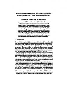
Preds/Interpolants y ≡2 1 x + y ≡2 0 x + y + z ≡4 0 x ≡4 0, y ≡4 0 4x + 2y + z ≡8 0 4x − 2y + z ≡222 0 x + y ≡3 0
VINT2 2.72s 0.83s 0.95s 1.1s 0.93s 0.54s -
1000
HNF (seconds)
Example ex1 ex2 ex4 ex5 ex6 ex7 forb1
100 10 1 0.1 0.01 0.01
0.1
1
10
100
1000
Yices Black-box Use (seconds)
(b) (a) Fig. 1. (a) Table showing the predicates needed and time taken in seconds. (b) Comparing Hermite Normal Form based algorithm and black-box use of Yices for getting proofs of unsatisfiability
is unreachable). The existing tools based on predicate abstraction and counterexample guided abstraction refinement (CEGAR) such as BLAST [9], SATABS [1] are not able to verify these programs. This is because the inductive invariant required for the proof contains LMEs as predicates, shown in the “Preds/Interpolants” column of Figure 1(a). These predicates cannot be discovered by the interpolation engine [15, 19] used in BLAST or by the weakest precondition based procedure used in SATABS. The interpolation algorithms described in this paper are able to find the right predicates by computing the interpolants for spurious program traces. Only one unwinding of the while loop suffices to find the right predicates in 6 out of 7 cases. We wrote similar programs in Verilog and tried verifying them with VCEGAR [2], a CEGAR based model checker for Verilog. VCEGAR fails on these examples due to its use of weakest preconditions. Next, we externally provided the interpolants (predicates) found by INT2 to VCEGAR. With the help of these predicates VCEGAR is able to show the unreachability of ERROR labels in all examples except forb1 (ERROR is reachable in the Verilog version of forb1). The runtimes are shown in “VINT2” column. M¨uller-Olm and Seidl [16] propose an abstraction technique that can infer linear invariants that are sound with respect to integer arithmetic modulo a power of 2. Their work provides an alternative way of verifying the programs listed in Figure 1(a). Proofs of Unsatisfiability (PoU) Algorithms: We obtained 459 unsatisfiable formulas (system of LDEs) by unwinding the while loops for C programs mentioned above. The number of LDEs in these formulas range from 3 to 1500 with 2 to 4 variables per equation. There are two options for obtaining PoU in INT2. a) Using Hermite Normal Form (HNF) (Section 5.1). We use PARI/GP [4] to compute HNF of matrices. b) By using a state-of-the-art SMT solver Yices 1.0.11 [3] in a black-box fashion (along the lines of [19]). Given a system of LDEs AX = B we encode the constraints that RA is integral and RB is not an integer by means of mixed integer linear arithmetic constraints (see [10]). The SMT solver returns concrete values to elements in R if AX = B is unsatisfiable. The comparison between (a) and (b) is shown in Figure 1(b). There is a timeout of 1000 seconds per problem. The HNF based algorithm is able to solve all problems, while the black-box usage of Yices cannot solve 102 problems within the timeout. Thus, the HNF based method is superior over the black-box use of Yices. Note that the interpolation algorithms proposed in our paper are independent of the algorithm used to generate the PoU. Any decision procedure that can produce PoU according to definitions 1, 3 can be used (we are not restricted to using HNF or Yices).
8
Conclusion
We presented polynomial time algorithms for computing proofs of unsatisfiability and interpolants for conjunctions of linear diophantine equations, linear modular equations and linear diophantine disequations. These interpolation algorithms are useful for discovering modular/divisibility predicates from spurious counterexamples in a counterexample guided abstraction refinement framework. In future, we plan to work on interpolating theorem provers for integer linear arithmetic and bit-vector arithmetic and make use of the satisfiability modulo theories framework. Acknowledgment. We thank Axel Legay and Jeremy Avigad for their valuable comments.
References 1. 2. 3. 4. 5. 6. 7. 8. 9. 10.
11. 12. 13. 14. 15. 16. 17. 18. 19. 20. 21.
SATABS 1.9 website, http://www.verify.ethz.ch/satabs/. VCEGAR 1.3 website. http://www.cs.cmu.edu/∼modelcheck/vcegar/. Yices 1.0.11 website. http://yices.csl.sri.com/. PARI/GP, Version 2.3.2, 2006. http://pari.math.u-bordeaux.fr/. Alexander Bockmayr and Volker Weispfenning. Solving numerical constraints. In A. Robinson and A. Voronkov, editors, Handbook of Automated Reasoning, pages 751–842. 2001. Alessandro Cimatti, Alberto Griggio, and Roberto Sebastiani. Efficient interpolation in satisfiability modulo theories. In TACAS, 2008. E. Clarke, O. Grumberg, S. Jha, Y. Lu, and H. Veith. Counterexample-guided abstraction refinement for symbolic model checking. J. ACM, 50(5), 2003. William Craig. Linear reasoning. a new form of the herbrand-gentzen theorem. J. Symb. Log., 22(3):250–268, 1957. Thomas A. Henzinger, Ranjit Jhala, Rupak Majumdar, and Kenneth L. McMillan. Abstractions from proofs. In POPL, pages 232–244. ACM Press, 2004. Himanshu Jain, Edmund M. Clarke, and Orna Grumberg. Efficient craig interpolation for linear diophantine (dis)equations and linear modular equations. Technical Report CMU-CS08-102, Carnegie Mellon University, School of Computer Science, 2008. Ranjit Jhala and Kenneth L. McMillan. A practical and complete approach to predicate refinement. In TACAS, pages 459–473, 2006. Deepak Kapur, Rupak Majumdar, and Calogero G. Zarba. Interpolation for data structures. In SIGSOFT ’06/FSE-14, pages 105–116. ACM, 2006. Daniel Kroening and Georg Weissenbacher. Lifting propositional interpolants to the wordlevel. In FMCAD, pages 85–89. IEEE, 2007. K. L. McMillan. Interpolation and sat-based model checking. In CAV, pages 1–13, 2003. K. L. McMillan. An interpolating theorem prover. In TACAS, pages 16–30, 2004. Markus M¨uller-Olm and Helmut Seidl. Analysis of modular arithmetic. ACM Trans. Program. Lang. Syst., 29(5):29, 2007. Greg Nelson and Derek C. Oppen. Simplification by cooperating decision procedures. ACM Trans. Program. Lang. Syst., 1(2):245–257, 1979. Pavel Pudl´ak. Lower bounds for resolution and cutting plane proofs and monotone computations. J. Symb. Log., 62(3):981–998, 1997. Andrey Rybalchenko and Viorica Sofronie-Stokkermans. Constraint solving for interpolation. In VMCAI, pages 346–362, 2007. A. Schrijver. Theory of linear and integer programming. John Wiley & Sons, NY, 1986. Greta Yorsh and Madanlal Musuvathi. A combination method for generating interpolants. In CADE, pages 353–368, 2005.