time–efficient reachability tests along the ancestor, descen- dant, and link axes to
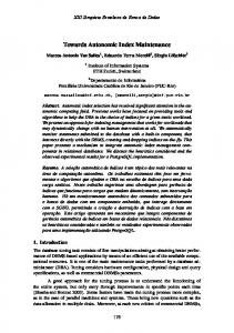
..... connections from the ancestors of u (including u) to the de- scendants of v ...
Efficient Creation and Incremental Maintenance of the HOPI Index for Complex XML Document Collections Ralf Schenkel Anja Theobald Gerhard Weikum Max-Planck-Institut f¨ur Informatik, Saarbr¨ucken, Germany {schenkel,atb,weikum}@mpi-sb.mpg.de
Abstract The HOPI index, a connection index for XML documents based on the concept of a 2–hop cover, provides space– and time–efficient reachability tests along the ancestor, descendant, and link axes to support path expressions with wildcards in XML search engines. This paper presents enhanced algorithms for building HOPI, shows how to augment the index with distance information, and discusses incremental index maintenance. Our experiments show substantial improvements over the existing divide-and-conquer algorithm for index creation, low space overhead for including distance information in the index, and efficient updates.
1 Introduction 1.1 Motivation For efficient evaluation of path queries on XML data (i.e., // conditions in XPath) appropriate index structures are called for such as DataGuides [13] and its many variants. However, prior work has mostly focused on index structures for path queries without wildcards, with poor performance for wildcard queries, and has not paid much attention to intra- or inter-document links (XPointer,XLink,ID/IDREF). In contrast, the HOPI index [26], which is based on the 2–hop cover of a graph [7], has been judiciously designed to handle path expressions over arbitrary graphs (i.e., not merely trees or tree-like DAGs) and to support the efficient evaluation of path queries with wildcards. The work in [26] did, however, leave several key issues open, regarding incremental updates to indexes and the support of ranked retrieval of XML documents. HOPI is very space-efficient, representing all transitive connections in less than ten percent of the space than a materialized transitive closure would need. However, this makes updates like
insertion or deletions of new XML documents, elements, and links more challenging. In the current paper we develop an efficient solution to these update operations that can be applied to a large fraction of updates. As for ranked retrieval, the need for approximate, similarity-driven, search on heterogeneous or non-schematic XML collections (e.g., in large intranets) has motivated various approaches to combining IR-style scoring and ranking techniques with XPathstyle querying [1, 9, 11, 15, 28], including our own XXL search engine [27, 29, 30]. One aspect of such scoring is to take into account the link distance between elements that are considered as matches to subqueries. In this paper, we extend the HOPI index to support fast retrieval of XML elements together with their distance, as an important building block for ranked retrieval of XML documents. In addition to addressing the above two key issues, this paper also reconsiders the efficient bulk construction of XML connection indexes. This is an important issue because of the need for 24x7 availability in virtually all applications (e.g., in business portals or intranet search engines) so that indexes need to be built without interrupting the service of queries. It matters whether an index can be built within an hour in a background process with small memory consumption and little interference with concurrent queries, or whether this takes a full day with high memory demand and adverse effects on the performance of the regular workload. The index build procedures developed in [26] provided a reasonably efficient solution using a graph partitioning approach with subsequent joining of partition-wise two-hop covers. The current paper significantly improves this method by using more intelligent techniques for forming partitions, choosing so-called center nodes for the twohop cover computations, and joining the resulting covers.
1.2 Related Work Path index structures for efficiently evaluating XML path queries have been intensively studied in the literature. The most efficient path indexes use encoding schemes for trees (e.g., [14, 34]), but are inherently limited to tree-structured
Proceedings of the 21st International Conference on Data Engineering (ICDE 2005) 1084-4627/05 $20.00 © 2005 IEEE
XML without links. There are some index structures that support collections with links, e.g. APEX [5], the Index Definition Scheme [18], the D(k) Index [23], and the M(k) Index [16], but they typically cannot efficiently support finding descendants for arbitrary queries, even though some of them can be tuned for frequently occuring queries. Most of the indexes can be augmented with distance information, but the papers do not explicitly deal with this issue as these indexes were not designed for XML retrieval systems where distance plays an important role. The FliX framework [25] has been designed for that purpose; it uses existing index structures, among them HOPI [26], as building blocks. The issue of maintaining path indexes has recently been discussed for the A(k) and 1-index [33]. Update-friendly index structures for tree-structured data are presented in [4, 8, 10, 17, 22, 32]. Besides our own work in [26], Sayed and Unland [24] also use the concept of a 2–hop cover to index connections in XML documents, but they do not cover the issues discussed in this paper.
1.3 Contributions and Outline This paper extends the existing HOPI index in the following important aspects:
all parent-child relationships between elements in d. Additionally, we maintain the set LI (d) ⊂ VE (d) × VE (d) of all intra-document links within d. The element-level graph GE (d) = (VE (d), EE (d)) has the same node set as the tree, but its edge set is extended by the intra-links, i.e., � (d) ∪ LI (d). EE (d) = EE A collection X = (D, L) of XML documents consists of a set D = {d1 , ..., dn } of documents together with the set L of inter-document links between documents in D, i.e., pairs of elements from different documents�that are connected via a link. We denote with L(X) := L∪ d∈D LI (D) the set of all links in the collection X. A subcollection X � = (D� , L� ) of a collection X = (D, L) consists of a subset D� of D and the subset L� of the links from L between documents in D� . In this paper, we denote the collection of XML documents known to the search engine as X = (D, L). The element-level graph G E (X) = (VE (X), EE (X)) for a collection X = (D, L) of XML documents has as vertex set the union of the elements of the documents in D, and as edge set the union of the edge sets of the element-level graphs for the documents plus the set L of inter-document links (see Fig. 1, ignoring the node labels for now). The document mapping function doc : V E (X) → D for a collection X = (D, L) maps vertices of the element-level graph of the collection to the document they originate in.
• We introduce a new, structurally recursive algorithm for joining partition covers that highly reduces the time needed to join the covers.
8
• We present a new algorithm for partitioning the document-level graph that takes the size of the transitive closure into account.
9
For an XML document d, we consider the element-level � (d)) where the vertex set VE (d) tree TE (d) = (VE (d), EE consists of all elements of d and the edge set represents
5 3
1
d2 d1
• We give algorithms for incremental index maintenance under insertions and deletions of documents, elements or edges.
2 Formal Model and Notation
4 2
• We show how to augment HOPI with distance information and how the building process has to be modified to efficiently create such an augmented index.
The rest of the paper is structured as follows. Section 2 introduces our formal model. Section 3 shortly reviews the HOPI index. Section 4 presents a new algorithm for efficient index creation. Section 5 shows how to augment the index with distance information. Section 6 discusses algorithms for incremental index maintenance. Section 7 experimentally evaluates our results.
Lin(u) = {...} u Lout(u) = {5,6,...}
7
6
v
d3
Lin(v) = {5,...} Lout(v) = { }
Figure 1. Element-level graph for a collection of three XML documents. Dashed lines denote document boundaries, thin arrows denote parent-child edges, strong arrows denote interdocument links, dashed arrows denote intradocument links. For vertices u and v, two-hop labels are shown (see Section 3).
In addition to the element-level graph, we maintain the document-level graph G D (X) = (D, ED (X)) with the documents as vertices and an edge (di , dj ) if there is a link (v, w) ∈ L such that doc(v) = di and doc(w) = dj . A weight function w assigns weights (real numbers greater or equal to 0) to both vertices and edges. Given a collection X = (D, L), a partition Pi =
Proceedings of the 21st International Conference on Data Engineering (ICDE 2005) 1084-4627/05 $20.00 © 2005 IEEE
(Di , Li ) of X is a subcollection of X with Li = {(u, v) ∈ L | doc(u) ∈ Di ∧ doc(v) ∈ Di }. A partitioning P (X) = ({P1 , ..., Pm }, LP ) of X is a set of disjoint partitions of X together with a set of links, such that ∪Di = D, � Li ∪ LP = L, and LP is disjoint with every Li . The partition map part : D → {P1 , ..., Pm } maps each document to its corresponding partition. Note that this model disregards the ordering of an element’s children and the possible ordering of multiple links that originate from the same element. The rationale for this abstraction is that we primarily address schema-less or highly heterogeneous collections of XML documents. In such a context, it is extremely unlikely that application programmers request accesss to the second author of the fifth reference and the like, simply because they do not have enough information about how to interpret the ordering of elements.
3 Foundations of HOPI 3.1 Two-Hop Covers A 2–hop cover of a graph G = (V, E) is a compact representation of connections in the graph that has been developed by Cohen et al. [7]. Let C(G) = (V, T (G)) the reflexive and transitive closure of G, i.e., T (G) = {(x, y)|there is a path from x to y in G} is the set of all connections in G. For each such connection (x, y) in G (i.e., (x, y) ∈ T ), we choose a node w on a path from x to y as a so-called center node and add w to a set L out (x) of descendants of x and to a set Lin (y) of ancestors of y. Now we can test efficiently if two nodes u and v are connected by a path in G by checking if Lout (u) ∩ Lin (v) = ∅. There is a path from u to v iff Lout (u) ∩ Lin (v) �= ∅; and this connection from u to v is given by a first hop from u to some w ∈ Lout (u) ∩ Lin (v) and a second hop from w to v, hence the name of the method. As an example consider the nodes u and v and their sets Lin and Lout shown in Figure 1. There is a path from u to v, because Lout (u) ∩ Lin (v) = {5} is not empty. For a node x, we say that L(x) = (Lin (x), Lout (x)) is the two-hop label or short label of x. A two-hop cover of G is a set of two-hop labels for each node in G that covers the connections in G, i.e., for each edge (x, y) ∈ T (G), Lout (x)∩Lin (y) �= ∅. We denote the two-hop cover as L = (Lin , Lout ). We define the size of a two-hop � cover as the sum of the sizes of all node labels: |L| = v∈V (|Lin (v)|+ |Lout (v)|).
3.2 Building a Two-Hop Cover Computing an optimal 2–hop cover (i.e., a cover whose size is minimal among all two-hop covers) is an NP–hard
problem. However, Cohen et al. introduce an approximation algorithm that we shortly review here. The input to the algorithm is the reflexive and transitive closure C(G) = (V, T (G)) of a graph G = (V, E); for simplicity, we simply write C instead of C(G) and T for T (G) in the remainder of this section. For a node w ∈ V , Cin (w) = {v ∈ V |(v, w) ∈ T } denotes the set of ancestors of w in G, Cout (w) = {v ∈ � V |(w, v) ∈ T } the set of descendants of w. For subsets Cin � of Cin (w) and Cout of Cout (w), the set � � � � , w, Cout ) = {(u, v) ∈ T |u ∈ Cin and v ∈ Cout } S(Cin � denotes the set of paths in G from nodes in Cin to nodes in � Cout that contain w. We say that w is the center of the set � � S(Cin , w, Cout ). The algorithm incrementally builds a two-hop cover, starting with an empty set L of labels for each node. It maintains the set T of yet uncovered connections which is initialized with T . In each iteration, the algorithm picks a � � ⊆ Cin (w) and Cout ⊆ Cout (w) and updates node w, Cin the cover as follows: � (w) : Lout (u) := Lout (u) ∪ {w} for all u ∈ Cin � (w) : Lin (v) := Lin (v) ∪ {w} for all v ∈ Cout � � Then S(Cin (w), w, Cout (w)) is removed from the set T � of uncovered connections and the iteration continues until T � = ∅, i.e., L is a two-hop cover for T . To decide which node to pick in order to arrive at a cover � with a small size, we consider for a node w and Cin and � � � � Cout as above the set S(Cin , w, Cout ) ∩ T that contains all � � to nodes in Cout that contain paths in G from nodes in Cin w and are not yet covered. The ratio
r(w) =
max
C � ⊆Cin (w) in � Cout ⊆Cout (w)
� � |S(Cin , w, Cout ) ∩ T �| � | + |C � | |Cin out
then describes the optimal relation between the number of connections via w that are not yet covered and the total number of nodes that lie on such connections. If we choose w with the highest r(w) among all nodes, we have to update the labels of only a small set of nodes while covering many of the uncovered connections, thus we get the most benefit for the increase in the size of L . � � , Cout for a given The problem of finding the sets Cin node w ∈ V that maximizes the quotient r(w) is equivalent to the problem of finding the densest subgraph of the socalled center graph of w. This undirected bipartite graph CGw = (Vw , Ew ) contains two nodes vin and vout for each node v ∈ V of the original graph. There is an undirected edge (uout , vin ) ∈ Ew if (u, v) ∈ T � is a not yet covered connection, u ∈ Cin (w), and v ∈ Cout (w). All isolated nodes are removed from Vw .
Proceedings of the 21st International Conference on Data Engineering (ICDE 2005) 1084-4627/05 $20.00 © 2005 IEEE
� The density δw of a subgraph CG�w = (Vw� , Ew ) is the average degree (i.e., number of incoming and outgoing � |/|Vw� |), and the densest subedges) of its nodes (δw = |Ew graph of Gw is the subgraph with the highest density. It can be computed by a linear-time 2–approximation algorithm which iteratively removes a node of minimum degree from the graph. This generates a sequence of subgraphs and their densities, the algorithm returns the subgraph with the highest density. The algorithm for computing a 2-hop cover chooses in each step the node w whose centergraph has the subgraph G�w with highest density among all nodes in V . From G�w , � � the sets Cin and Cout are derived and used for updating the cover. In addition to this basic algorithm from Cohen et al., we proposed in [26] some extensions that drastically reduce the runtime for the algorithm (without, however, reducing its theoretical complexity). Our first extension aimed at reducing the number of computations of densest subgraphs. It is easy to see that the density of the densest subgraph of a centergraph will not increase if some connections are removed. We therefore precompute the density δw of the densest subgraph of the center graph of each node w of the graph G when the algorithm starts and insert each node w in a priority queue with δw as priority. In each step, we extract the node with highest priority from the queue and check if its density is still correct; if not, we push it back with the new density and extract the next node. We repeat this until we find a node with correct density which is then used to update the cover. Using this queue, we have to recompute the densest subgraphs for only few instead of all nodes. As we also showed that the initial center graphs are always their own densest subgraph, we do not have to explicitly compute the initial densest subgraph of each node, but can immediately use the density of the inital center graphs. This saves some time for precomputation.
3.3 Divide-and-Conquer Algorithm for Index Building Since materializing the transitive closure as the input of the 2–hop-cover computation can be very critical in terms of memory consumption, we proposed in [26] a divide-andconquer technique based on a partitioning of the documentlevel graph for the collection X . Our technique works in three steps: (1) It computes a partitioning P = ({P1 , ..., Pm }, LP ) of GD (X ) such that the size of the transitive closure of each partition can be computed in-memory. (2) It computes the transitive closure and the 2–hop cover for each partition and stores the 2–hop cover in the database. (3) It merges the partition covers by adding cover entries
a
u
v
d
Figure 2. Integrating the link u → v into the cover. Node v serves as a center node for all newly created connections, so it is added to Lout of u, all ancestors a of u in the current cover, and v itself, and to Lin of v and all descendants d of v in the current cover.
for links between documents in different partitions, yielding a 2–hop cover for the entire graph. To build the partitioning, the weight of a node di ∈ VD (X ) is set to the number of elements of di , and the weight of an edge (di , dk ) ∈ ED (X ) is set to the number of links from di to dk . We limit the number of nodes such that the transitive closure of each partition can be carried out in-memory by conservatively limiting the sum of node weights within a single partition and minimizing the weight of cross-partition edges. To connect the partition covers, we start with the (component-wise) union L of the partition covers and iterate through the cross-partition links. For each such link u → v, we choose v as center node for all newly created connections from the ancestors of u (including u) to the descendants of v (including v) (see Fig. 2) and extend L in the following way: We add v to Lout of u, all ancestors a of u in the current cover, and v itself, and add v to Lin of v and all descendants d of v in the current cover. Here, ancestors and descendants are computed using the cover that was computed so far. This incremental algorithm eventually creates a cover that reflects all connections in GE (X ).
3.4 Database-Backed Implementation As we aim at very large, dynamic XML collections, we implemented HOPI as a database-backed index structure, by storing the 2–hop cover in database tables and running SQL queries against these tables to evaluate queries. We need two tables LIN and LOUT that capture Lin and Lout : CREATE TABLE LIN(ID INID
NUMBER(10), NUMBER(10));
CREATE TABLE LOUT(ID NUMBER(10), OUTID NUMBER(10));
Here, ID stores the ID of the node and INID/OUTID store the node’s label, with one entry in LIN/LOUT for each entry in the node’s corresponding Lin /Lout sets. To minimize the number of entries, we do not store the node itself as INID or OUTID values.
Proceedings of the 21st International Conference on Data Engineering (ICDE 2005) 1084-4627/05 $20.00 © 2005 IEEE
For efficient evaluation of queries, additional database indexes are built on both tables: a forward index on the concatentation of ID and INID for LIN and on the concatentation of ID and OUTID for LOUT, and a backward index on the concatentation of INID and ID for LIN and on the concatentation of OUTID and ID for LOUT. In our implementation, we store both LIN and LOUT as index-organized tables in Oracle sorted in the order of the forward index, so the additional backward index doubles the disk space needed for storing the tables. To test if two nodes identified by their ID values ID1 and ID2 are connected, the following SQL statement would be used if we stored the complete node labels (i.e., did not omit the nodes themselves from the stored Lin and Lout labels):
X = (D, L) of XML documents, the partition-level skeleton graph (PSG) S(P ) = (VS (P ), ES (P )) consists of the set VS (P ) of nodes that are sources or targets of a link in LP . Its set of edges ES (X) consists of the set LP of links plus additional edges that represent connections of link targets and sources within the same partition.
7 8
4 Efficient Index Creation The original implementation of HOPI as presented in [26] already gives very good results in terms of compression of the transitive closure, but the time needed to build the index is a significant cost. In this section we present enhancements of HOPI’s original divide-and-conquer algorithm for index building, namely (1) a structurally recursive algorithm for joining partition covers, (2) a link-aware algorithm for preselecting center nodes, and (3) some enhancements to the partitioning process.
Definition 1 (Partition-Level Skeleton Graph). Given a partitioning P = ({P1 , ..., Pm }, LP ) of a collection
7
1
2
3 6
P2 P1
Figure 3. Partitioning (left) and corresponding PSG (right) for the element-level graph shown in Figure 1. In the partitioning, dark arrows represent cross-partition links; in the PSG, solid arrows represent cross-partition links, dashed arrows represent connections between link targets and sources within the same partition. The new algorithm for building a 2–hop cover starts by building a partitioning P = ({P1 , ..., Pm }, LP ) such that the transitive closure for each partition fits into main memory. We then build, for each partition Pi , a corresponding 2–hop cover H i (all these computations can be done concurrently). Next we construct the partition-level skeleton graph S(P ) and build a 2–hop cover H = (Hin , Hout ) for it by recursively applying the algorithm; this may include partitioning the PSG. From this cover, we compute a supˆ by copying entries from H to partitionplementary cover H level ancestors and descendants of the nodes in S(P ). More ˆ and set detailed, we start with an empty cover H ˆ out (a) = H ˆ out (a)∪ • for each link source s ∈ VS (P ), H Hout (s) for each ancestor a of s in partition part(s), and ˆ in (d) = H ˆ in (d) ∪ • for each link target t ∈ VS (P ), H Hin (t) for each descendant d of t in partition part(t).
4.1 Efficiently Joining Partition Covers The main reason for the large time needed to build HOPI is the incremental algorithm to join partition covers. In this section, we propose a new, structurally recursive algorithm for joining partition covers that builds a new graph consisting essentially of the cross-partition links and computes a 2– hop cover for this graph. The resulting cover is then joined with the partition covers into the final cover. The graph that is built by this algorithm is the so-called partition-level skeleton graph (PSG) (see Fig. 3):
8 5
1
SELECT COUNT(*) FROM LIN, LOUT WHERE LOUT.ID=ID1 AND LIN.ID=ID2 AND LOUT.OUTID=LIN.INID
This query performs the intersection of the Lout set of the first node with the Lin set of the second node. Whenever the query returns a non-zero value, the nodes are connected. As we do not store the node itself in its label, the system executes some simple additional queries (see [26] for details); for ease of presentation, we do not mention these additional queries here. Similar queries are used to find descendants or ancestors of a fixed node.
4 2
Here, ancestors and descendants are computed using the covers H i for the partitions. Then, the (component-wise) ˆ forms a 2–hop cover for GE (X). union of the H i , H, and H The following theorem shows the correctness of this algorithm: Theorem 1. The 2–hop cover L formed by unifying the H i , ˆ is a 2–hop cover for G E (X). H, and H Proof. We have to show that i) all connections in GE (X) are covered, and ii) the cover does not reflect nonexisting connections.
Proceedings of the 21st International Conference on Data Engineering (ICDE 2005) 1084-4627/05 $20.00 © 2005 IEEE
(i) We consider an arbitrary connection (u, v) in GE (X). If u and v are from the same partition, this connection is covered by the partition cover. If they are from different partitions, we follow an arbitrary path u = x0 , x1 , ..., xn = v from u to v in GE (X) and consider the node xi where the path leaves u’s partition for the first time (i.e., part(xi ) = part(u), but part(xi+1 ) �= part(u)) and the node xk where the path finally enters v’s partition (i.e., part(xk ) = part(v)), see Fig. 4. Both xi and xk are nodes in the PSG, and we can construct a path from xi to xk in the PSG, hence they are connected, so Hout (xi ) ∩ Hin (xk ) �= ∅. Now u is an ancestor of xi in u’s partition and v is a descendant of xk in v’s partition, so by construction of L, Lout (u) ⊇ Hout (xi ) and Lin (v) ⊇ Hin (xk ), hence Lout (u) ∩ Lin (v) �= ∅ and L covers the connection (u, v). A similar argument can be applied if one or both of u and v are on the partition border. (ii) Assume that there are u, v ∈ VE (X) such that Lout (u) ∩ Lin (v) �= ∅, but there is no path from u to v in GE (X); select any c ∈ Lout (u) ∩ Lin (v). Now Lout (u) is part(u) ˆ out (u). As the first the union of Hout (u),Hout (u), and H two are part of valid 2–hop covers, there is always a path from u to c if c is contained in one of them. If c is contained ˆ out (u), there is a link source s such that u →∗ s in u’s in H partition and u →∗ c in the partition-level skeleton graph S(P ), hence by construction of S(P ) there is a path from u to c in GE (X). By the same argument, there is a path from c to v, so the assumption that u and v are unconnected must be wrong.
u
xi
xk
v
Figure 4. Illustration for the proof of Theorem 1. u and xi are in one partition, xk and v are in another partition, and there is a path u →∗ xi →∗ xk →∗ v. From the proof of Theorem 1 it is evident that, instead of considering a cover for the complete PSG, it is sufficient to consider only connections between sources and targets of cross-partition links. (Remember that we reduced an arbitrary connection between two nodes to a connection between a link source and a link target.) Such a cover is typically smaller than the cover H. We consider the following ¯ that uses targets of cross-links as center nodes: cover H ¯ out (s) := {t | t ∈ • for all link sources s ∈ VS (P ), H ∗ VS (P ) link target and s → t in S(P )}
¯ in (t) := {t} • for all link targets t ∈ VS (P ), H ¯ is a cover for the set of connecIt is easy to show that H tions from link sources to link targets in S(P ). Even though this cover may not be the smallest one, it can be computed quickly from the PSG using an adapted transitive closure algorithm. If the PSG is too large, we partition it into several partitions, making sure that (1) we can compute the partial cover for each partition in memory, and (2) every edge between two partitions starts at a link target in the original PSG and ends at a link source (by moving nodes between partitions until this property holds). The partition covers are then connected by, for each cross-partition edge (t, s), ¯ out (a) for each ancestor a of t that is a ¯ out (s) to H adding H link source. The following corollary summarizes our new algorithm for joining partition covers: Corollary 1. The 2–hop cover L formed by unifying the ¯ and H ˆ is a 2–hop cover for G E (X). H i , H,
4.2 Selection of Center Nodes When computing the cover for a single partition, HOPI considers only intra-partition edges when choosing center nodes. However, the partition covers will be joined afterwards, and both the existing algorithm for joining the covers (see Section 3.3) and the new algorithm (see Section 4.1) use link targets as center nodes. It may therefore be useful to consider link targets as center nodes when building partition covers, before starting the normal cover building. Our new algorithm maintains a separate list that contains only link targets. It then creates cover entries for all connections for which the link targets can be center nodes, removes them from the transitive closure, and computes cover entries for the remaining connection. This helps to reduce the size of the final cover, as there are fewer redundant entries.
4.3 Building the Initial Partitioning When building the initial partitioning, HOPI’s randomized partitioner conservatively limits the number of nodes in the partition such that the transitive closure of the partition is small enough to fit into memory. This misses opportunities as it completely ignores the structure of the graph, yielding partitions that are too small most of the time. Our new algorithm therefore computes, while incrementally building the partition, the transitive closure of the partition and continues with the next partition when the transitive closure is as large as the available memory. This allows much more connections to be covered by the partition covers and reduces the number of cross-partition links, yielding a smaller overall cover.
Proceedings of the 21st International Conference on Data Engineering (ICDE 2005) 1084-4627/05 $20.00 © 2005 IEEE
In addition to this optimization, the current choice of the edge weights may not be perfect. HOPI uses the number of links between documents as edge weight for partitioning. It may be better to determine how many connections are made using a link (by counting the number of ancestors A of the link source and the number of descendants D of the link target and then using either A ∗ D or A + D as edge weight; here, A ∗ D corresponds to the number of connections over this link, and A + D corresponds to the number of nodes connected over this link. This gives more weight to edges in the ”center” of the graph, which may reduce the additional center nodes introduced when joining the partition covers. To compute the number of ancestors and descendants, we make use of the skeleton graph S(X) that has as nodes elements that are sources or targets of inter-document links. Its edges are the links and, for each link target u, an edge to each link source v in the same document, provided u and v are connected within that document. Definition 2 (Skeleton Graph). Given the element-level graph GE (X) = (VE (X), EE (X)) for a collection X = ({d1 , . . . , dn }, L) of XML documents, the Skeleton Graph S(X) = (VS (X), ES (X)) consists of the set VS (X) := VSS (X)∪VST (X) of nodes where VSS (X) := {v ∈ VE (X) | (v, x) ∈ L(X)} is the set of link sources and VST (X) := {v ∈ VE (X) | (x, v) ∈ L(X)} is the set of link targets. Its set of edges ES (X) := L(X) ∪ {(v, x) ∈ VST (X) × VSS (X) | doc(v) = doc(x) and v → ∗ x in TE (doc(v))} consists of the set L(X) of links plus additional edges that represent connections of link targets with link sources within the same element-level tree. (1,10)
(2,8)
(3,1)
(1,8)
8
7
4
5
9
1
2
3
6
(3,1)
(4,4)
(4,1)
(5,2)
(4,1)
Figure 5. Skeleton graph for the elementlevel graph shown in Figure 1. Solid arrows correspond to links, dashed arrows to connections of link targets and sources within the same element-level tree. Each node is annotated with its number of ancestors and descendants in the element-level tree of its document. We annotate each node x in S(X) with its number of ancestors anc(x) and descendants desc(x) within the elementlevel tree of its document (see Fig. 5); this can be easily derived if we maintain pre- and postorder values for each node
until we have built the HOPI index. The (approximated) number of ancestors and descendants of each node can then be computed by a breadth-first traversal of S(X) starting at each node: Whenever the traversal starting at node x traverses along cross-document link (u, v), the overall number of descendants D(x) of x is increased by desc(v); whenever a link (u, v) to a link source is traversed, the overall number of ancestors A(v) of v is increased by anc(x). As S(X) may contain long paths, the computation is limited to paths of a certain length, hence the resulting numbers are only approximates of the real numbers.
5 Reflecting Distance Information 5.1 Representing Distance in the Database Lookups on connection lengths and queries for limitedlength paths between nodes with certain tags are important in the context of our XXL search engine for ranking results of information-retrieval-style queries, e.g., of the kind //∼book//author. For such queries, the ranking of entire XML paths may take into consideration not only the similarity of the data tags to the ones in the query (e.g., the ontological similarity of book to monography or publication) but also the length of the connections between qualifying elements. For example, a path where an author element is found far away from a book element should be ranked lower than an author that is a child or grandchild of a book. To enable ranking of results by distance, we additionally store distance information with the node labels, i.e., the minimal number of edges that some ancestor or descendant node is away from a center node. This information can be included in the 2-hop cover by adding the distance to the center node. We store this distance in the LIN and LOUT tables as an additional attribute DIST. Then, to test how long the shortest path between two nodes with IDs ID1 and ID2 is, we run the SQL query SELECT MIN(LOUT.DIST + LIN.DIST) AS B FROM LIN, LOUT WHERE LOUT.ID=ID1 AND LIN.ID=ID2 AND LOUT.OUTID=LIN.INID
Note that the minimum operator is necessary because paths over center nodes may have different lengths, but we are only interested in the shortest path.
5.2 Building a Distance-Aware 2–Hop Cover The existing algorithm for index building has to be slightly adapted for building a distance-aware cover. The input transitive closure and the resulting cover entries are augmented with distance information, e.g., entries in Lin (x) of a node x are now pairs (y, dist(x, y)) with dist(x, y) representing the shortest distance of x and y. The main modification is that a center node w can only cover the connection
Proceedings of the 21st International Conference on Data Engineering (ICDE 2005) 1084-4627/05 $20.00 © 2005 IEEE
(u, v) if w is on a shortest path from u to v, otherwise it cannot reflect the correct distance of u and v. This additional test is added to the construction of the center graph for w, where we add the edge u → v only if the distance of u and v is the same as the sum of the distances from u to w and from w to v. While this modification is sufficient to correctly build the index, it renders one of our initial optimizations useless: Initial center graphs are no longer complete, hence our estimation of the initial maximal density is way off, leading to repeated reinsertions of nodes. If we knew the number of edges E in the initial center graph, a better estimation for the maximal density of a subgraph would be √ E E √ = 2 2· E (the maximal density is achieved when the number of nodes on both sides is balanced and the graph is as complete as possible.) However, it turns out that exactly computing the number of edges of each initial center graph is expensive: if the center node has a ancestors and d descendants, we have to test a · d candidate connections if they correspond to a shortest path. Even though each of these tests requires constant time, the huge number makes this infeasible. To solve this, we apply a sampling algorithm that checks at most 13,600 randomly chosen candidate edges of the center graph for existance. From this preliminary estimation e� for the fraction of edges that really exists, we compute the 98% confidence interval [2, 21] (which has at most length 0.02 as we took 13,600 samples) and take the upper bound of the interval as our estimation E for the fraction of edges present in the graph. By construction, the probability that the fraction of edges present in the center graph is larger than E is less than 0.01, which is tolerable (especially if we consider that E serves as input for a much coarser approximation later). In our experiments, the initially estimated maximal density never exceeded the real maximal density.
6 Incremental Index Maintenance We are interested in dynamic XML data collections such as large intranets (e.g., large companies or universities) or federations of Web sources (e.g., bioinformatics sources). In such environments updates to existing documents may lead to insertions or deletions of edges in the XML graph, and entire documents can be added or removed. These changes must be reflected in the HOPI connection index in an incremental manner, without having to recompute the entire index from scratch. This section discusses our incremental algorithms for index maintenance: insertions, deletions, and modifications of nodes and edges. Over time, the space efficiency of the 2–hop cover that HOPI maintains may degrade. Then occasional rebuilds of the index may be
considered, using the efficient algorithm presented in Section 4. Note that the algorithms presented in the following can be applied also for distance-aware covers, even though we restrict the discussion to connection indexing for simplicity.
6.1 Insertions Reflecting new nodes or edges in the HOPI index and especially in its associated 2–hop cover L is straightforward. Adding an isolated node is trivial, as it requires no additions to the cover. A new edge (u, v) between two existing nodes u and v can be inserted by the same method that was used to add a link between partitions discussed in Section 3.3, i.e., considering v as center node for all newly created connections and add v to Lout (a) of all ancestors a of u including u and to Lin (d) for all descendants of v. A new document with outgoing and incoming links can be inserted by considering the document as a new partition, computing the 2–hop cover for this partition and applying the (old) algorithm for merging partitions discussed in Section 3.3.
6.2 Deletions Deleting an isolated node requires no special means, but deleting edges or entire documents is more complicated. For lack of space, we discuss only how to incrementally delete a document. A similar algorithm can be applied for deleting a single edge from the index. = Given the element-level graph GE (X) (VE (X), EE (X)) for a collection X = ({d1 , . . . , dn }, L) of XML documents and a 2-hop cover L = (Lin , Lout ) for the transitive closure C(GE (X)) = (VE (X), T (GE (X))) of GE (X), we want to remove the entire document di from the graph and compute a 2-hop cover L� that reflects the connections in the transitive closure C � (GE (X)) of GE (X) after removing di . To keep notation simple, we omit the parameter GE (X) of C, C � , T and T � in the future. The key problem is to decide which connections have to be removed from C in order to arrive at C � , because even if the center for a connection is in VE (di ), there may be another path between these nodes that does not contain a node from VE (di ), so that the connection must not be dropped. On the other hand, there may be nodes that are connected only through a path that contains nodes from VE (di ) but where the center node chosen for this connection is not from VE (di ). We now present two incremental algorithms that, given L, generate a new 2–hop cover L� that reflects the remaining connections. The first algorithm runs faster but can be applied only in special cases, whereas the second, general-purpose, algorithm requires more time.
Proceedings of the 21st International Conference on Data Engineering (ICDE 2005) 1084-4627/05 $20.00 © 2005 IEEE
1
2
3
5 7
4 6
8
9
Figure 6. Separating vs. non-separating nodes. Document 6 separates the documentlevel graph, document 5 does not.
To decide if we can apply the first algorithm, we consider the document-level graph GD (X) and denote by Anc(di ) the ancestors of di in GD (X) and by Desc(di ) its descendants. We say that di separates GD (X) if for every a ∈ Anc(di ) and d ∈ Desc(di ), a and d are connected only through paths that contain di . In other words, if we remove di from GD (X), a and d are no longer connected (see Fig. 6 for an example). We denote by VA the elements of documents in Anc(di ) and by VD the elements of documents in Desc(di ). Now we can show the following theorem on which our first algorithm builds: Theorem 2. If di separates GD (X), we can modify the 2–hop cover L for G E (X) into a 2–hop cover L � = (L�in , L�out ) that covers all connections in G E (X) after removing all nodes of V E (di ) as follows: for all a ∈ VA set L�out (a) := Lout (a) \ (Vdi ∪ VD ) for all d ∈ VD set L�in (d) := Lin (a) \ (Vdi ∪ VA ) Proof. To show that L� covers all remaining connections after removing di from GE (X), we have to show that (1) each connection is covered and that (2) L� does not reflect nonexisting connections. (1) Assume that there is a connection (u, v) after removing di from GE (X) that is not covered by L� . As di separates GD (X), there has been no path u →∗ v in GE (X) that contained nodes from VE (di ). Removing di does not create new connections and L is a 2–hop cover for connections in GE (X); so L covers (u, v), i.e., Q := Lout (u) ∩ Lin (v) �= ∅, and we remove the nodes in Q when we create L�out (u) and L�in (v). Without loss of generality assume we remove q ∈ Q from Lout (u), so u ∈ VA and there has been a path u →∗ q →∗ v before removing di from GE (X) because of the way we choose center nodes. Then q was either from VE (di ) or from VD . But q cannot be from VE (di ) because we just showed that no such paths exist, and by the same argument no nodes on the path can be in VE (di ). So q ∈ VD , but then there is a path from a node in an ancestor of di to a node in a descendant of di
in GD (X) after removing di , which is a contradiction to di separating GD (X). (2) Assume that there are nodes u, v ∈ VE (X) \ VE (di ) such that Q� := L�out (u) ∩ L�in (v) �= ∅, but u and v are not connected in GE (X) after removal of di . As L is a 2–hop cover for connections in GE (X) and L� is a subset of L, u and v must have been connected in GE (X) before removing di . Because they are no longer connected, each path u →∗ v in GE (X) must have included at least one node from VE (di ), so u ∈ VA and v ∈ VD . Consider an arbitrary q ∈ Q� , then q ∈ L�out (u) ⊆ Lout (u). Then either q ∈ VA , q ∈ VE (di ), or q ∈ VD . But q cannot be in VE (di ) or VD , because u ∈ VA and our algorithm deletes all such nodes from L� , so q ∈ VA must hold. On the other hand, q ∈ L�in (v) must also hold, so we can analogously show that q ∈ VD , which is a contradiction. Note that di separating GD (X) is sufficient for our algorithm to work, but not necessary. Even though there is a connection from an ancestor a to a descendant d of di in GD (X), the cover resulting from applying our algorithm may still be correct. The separation criterion therefore serves as an efficient test for whether we can simply drop the deleted document or need to take additional measures. When di does not separate GD (X), we have to partially reconstruct the transitive closure, as we do not know which connections will get lost when deleting di . However, we know that candidate connections that may possibly be lost start at nodes that are connected to a node in VE (di ). To determine which nodes are reachable from them after removing di , our iterative algorithm for computing the new transitive closure Cˆ starts with the nodes from the set � } S := {u ∈ VE (X)|∃d ∈ VE (di )such that(u, v) ∈ EX as seed and computes all nodes reachable from there. As the set of seed nodes is typically much smaller than the set of all nodes, the partial recomputation is typically much faster than recomputing the complete transitive closure for ˆ we compute the 2-hop cover L ˆ GE (X). Once we have C, ˆ Next, we define the sets Adi ⊆ VE (X) of ancestors for C. of the nodes VE (di ) and Ddi ⊆ VE (X) of descendants of nodes in VE (di ) as Adi Dd i
:= :=
{a|∃v ∈ VE (di ) such that (a, v) ∈ T } {d|∃v ∈ VE (di ) such that (v, d) ∈ T }
(note that VE (di ) is a subset of both sets) and set L� := ˆ except for the following nodes: L∪L for all a ∈ Adi : L�out (a) for all d ∈ Ddi : L�in (d)
:= :=
ˆ out (a) L ˆ in (d) (Lin (d) \ Adi ) ∪ L
This step removes from L all information about connections through nodes in VE (di ) and adds information about connections that were “accidentally” dropped by adding the
Proceedings of the 21st International Conference on Data Engineering (ICDE 2005) 1084-4627/05 $20.00 © 2005 IEEE
ˆ The following theonewly computed information from L. rem shows the correctness of this algorithm.
Coll. DBLP INEX
Theorem 3. The 2-hop cover resulting from applying the above algorithm represents exactly the connections in GE (X) after removing di . Proof. To show that L� covers all remaining connections after removing di from GE (X), we have to show that (1) each connection is covered and that (2) L� does not reflect non-existing connections. (1) Assume that (u, v) is a connection in GE (X) after removing di , so there is a path u →∗ v without any node from VE (di ). If u �∈ Adi , the algorithm didn’t modify Lo ut(u) and the center node for the connection hadn’t been chosen from VE (di ) before, so Li nv still contains the center node and the connection is reflected in L� after the modification. If u ∈ Adi , then the newly computed transitive closure Cˆ contains the connection and therefore the newly computed ˆ covers it. As the labels from L ˆ are added to 2–hop cover L ˆ all nodes and L does not contain any labels from VE (di ), L� covers this connection, too, so there cannot be a connection uncovered by L� . (2) Assume that there are nodes u, v ∈ VE (X) \ VE (di ) such that Q� := L�out (u) ∩ L�in (v) �= ∅, but u and v are not connected in GE (X) after removal of di . We choose an arbitrary q ∈ Q� and show that there are paths u →∗ q and q →∗ v in GE (X) after removing di no matter how L�out (u) and L� in(v) have been constructed, so u and v are connected. ˆ out (u), First consider u. If u ∈ Adi , then L�out (u) = L ∗ ˆ so u → q by the way we chose the center nodes for L. ˆ If u �∈ Adi , then either q ∈ Lout (u) (same as before) or q ∈ Lout (u) and there was a path u →∗ q in GE (X) before removing di without a node from VE (di ), so u and q are still connected after removing di . Next consider v. If v �∈ Ddi , there has been a path q →∗ v in GE (X) without any nodes from VE (di ) in GE (X) before removing di that still exists after removing di , so q and v are still connected. If q �∈ Ddi , either ˆ ˆ in (v) and q and v are connected by construction of L, q∈L or q ∈ Lin (v) but q is not an ancestor of a node in VE (di ), so the path q →∗ v that existed in GE (X) before removing di still exists after removing di . Putting everything together, we have shown that our assumption that the update cover reflects a non-existing connection is false.
6.3 Modifications When an existing document is modified (e.g., restructured so that many edges are added or removed), HOPI can simply drop the complete document and reinsert the modified version using the algorithms of the previous subsec-
# docs 6,210 12,232
# els 168,991 12,061,348
# links 25,368 408,085
size 13.2MB 534MB
Table 1. Important features of our collections of XML documents.
tions. Alternatively, it may be more efficient to analyze the modifications of the document, e.g. using XDiff [31] or XYDiff[6], and perform the corresponding insertions and deletions of edges and nodes.
7 Experimental Results 7.1 Setup In this section, we experimentally evaluate the algorithms for index building and index maintenance with two sets of XML documents: (1) a subset of 6,210 publications from important conferences and journals of the DBLP collection [20] where we created a separate XML document for each publication and added XLinks that correspond to citations1 , and (2) the INEX collection [12, 19, 27] as an example for a tree-structured collection without inter-document links. Table 1 summarizes important features of the collections. Note that we do not provide experiments about query performance as this was already covered in [26] and is not in the focus of this paper. We implemented HOPI in Java as an index for our XXL Search Engine [29, 30, 27]. All our experiments were run on a 64 processor Sun Fire-15000 server with 180 gigabytes of RAM, but we used only a limited amount of memory and a limited number of CPUs for our experiments. We used an Oracle 9.2 database server running on a Windows-based machine with two 3GHz Pentium IV CPUs, 2GB of RAM, and a 4-way RAID-0 SCSI hard disk array.
7.2 Index Size and Build Time We first investigated the size of indexes generated by our new algorithms and the time to build them, compared to the old algorithm from [26]. We give a thorough experimental analysis for the smaller DBLP dataset and discuss the numbers for INEX at the end of this section. The transitive closure for the subset of DBLP consists of 344,992,370 connections. As a baseline, we computed a two-hop cover for this set without partitioning. This cover had 1,289,930 entries and took 45 hours and 23 minutes and 1 Note that in contrast to our earlier work [26], this collection contains much more links, so the absolute numbers cannot be compared.
Proceedings of the 21st International Conference on Data Engineering (ICDE 2005) 1084-4627/05 $20.00 © 2005 IEEE
about 80 gigabytes of RAM to compute. Storing this cover in a database requires 5,159,720 integer numbers (two per entry in the table and another two in the backward index, see Section 3.4) compared to 1,379,969,480 for storing the transitive closure together with a backward index for answering ancestor queries, yielding a compression factor of about 267. Even though this is an impressive compression ratio, time and space requirements make this algorithm infeasible. The ”real” baseline for our experiments is therefore our old divide-and-conquer algorithm from [26] that represented these connections with 15,976,677 entries, yielding a compression ratio of about 21.6, and required 3 hours 10 minutes to compute it, where most of the time was spent joining the covers. To assess the quality of our new algorithm for joining partition covers, we tried the combination of HOPI’s existing partitioning algorithm with different partition sizes (denoted as Px, meaning a size limit of x · 104 nodes) and our new algorithm for cover joining; the results are shown in Table 2. All runs used only a single CPU, and all runs except P50 used less than one gigabyte of memory. The best results (P5 and P10) reduced the cover size by nearly 40% and the time by a factor of 10–15, so the new algorithm gives a great benefit. Runs with larger partition sizes (P20 and P50) generate more compact partition covers, but the joining algorithm adds more entries to the covers (as each link source and target has more ancestors and descendants because the partitions are larger). Inspired from these results, we also tried the ”naive” partitioning where each document forms a partition, but the results were not exactly convincing. Next we examined the effect of our new partitioning algorithm and the new edge weights from Section 4.3. It turned out that the new partitioning algorithm in combination with edge weights set to A*D gave similar results to the old partitioning algorithm, while the other combinations were not as good. Results from four runs are also depicted in Table 2 (denoted as Nx, meaning a size limit of x·105 connections). As the new algorithm creates partitions with a similar size of the transitive closures, cover computation takes roughly the same amount of time for each partition. Thus when distributed over n CPUs, this algorithm can achieve a speedup close to n, whereas the time with the old partitioner would be limited by the time to compute the cover for the largest partition. The new algorithm that preselects center nodes that are targets of cross-partition links gave some decrease in cover size, but the effects were marginal (about 10,000 entries less than the standard algorithm). For the INEX collection, the resulting cover has 33,701,084 entries and took slightly less than four hours to compute. We were not able to compute the size of the transitive closure due to space restrictions, but less than three index entries per node seems to be quite efficient.
algorithm baseline P5 P10 P20 P50 single N10 N25 N50 N100
time 11,400 820.8s 1,198.2s 2,286.8s 7,835.8s 22,778.0 1,359.7s 2,368.3s 3,635.8s 6,118.9s
size 15,976,677 9,980,892 10,002,244 11,646,499 12,033,309 12,384,432 9,999,052 10,601,986 10,274,871 12,777,218
compression 21.6 34.6 34.5 29.6 28.7 27.9 34.5 32.5 33.6 27.0
Table 2. Index build time and size with the baseline algorithm (top) and with the new algorithm for cover joining with different partitioning algorithms and partition size limits.
7.3 Index Maintenance Out of the 6,210 documents in the small DBLP collection, about 60% separate the collection, so we can apply the simple deletion algorithm. Testing if a document separates the collection takes 2 seconds on average, deleting the document afterwards about 13 seconds. When a document does not separate the collection, deleting it is more expensive, depending on the number of its ancestors and descendants in the document-level graph. In our experiments, deleting of documents with many connected documents was actually more expensive for some documents than rebuilding the complete cover, as it included recomputing the cover for a large fragment of the transitive closure (up to 5% for some documents). However, we do not yet apply our divide-and-conquer algorithm here, so we expect this to change in the future. For the INEX collection, each document separates the collection because there are no inter-document links. In such a setting, documents can be efficiently deleted using the optimized algorithm.
8 Conclusions and Future Work The algorithms presented in this paper add important functionality to the HOPI index. The new structurally recursive algorithm for index building improves time for index building by an order of magnitude compared to the existing algorithm of [26] while at the same time reducing index size. Additionally the index can be augmented with distance information, and efficient updates are supported for a large fraction of the documents.
Proceedings of the 21st International Conference on Data Engineering (ICDE 2005) 1084-4627/05 $20.00 © 2005 IEEE
Our future work with HOPI will focus on the following tasks: • We plan to investigate more general concepts of connectivity and structural similarity like those discussed in [3]. • We will employ HOPI in the FliX framework [25] and examine for which (sub-)collections HOPI is best suited and when other indexes perform better, using measures from graph theory and information theory. • As indexing connections in XML collections is not the only application for compressing the transitive closure of a graph, we will consider applications of this technique in other scenarios.
References [1] S. Al-Khalifa, C. Yu, and H. V. Jagadish. Querying structured text in an XML database. In SIGMOD 2003, pages 4–15, 2003. [2] A. Allen. Probability, Statistics, and Queueing Theory with Computer Science Applications. Academic Press, 1990. [3] S. Amer-Yahia et al. Tree pattern relaxation. In C. S. Jensen et al., editors, EDBT 2002, pages 496–513, 2002. [4] Y. Chen et al. L-Tree: a dynamic labeling structure for ordered XML data. In DataX Workshop, 2004. [5] C.-W. Chung et al. APEX: An adaptive path index for XML data. In SIGMOD 2002, pages 121–132, 2002. [6] G. Cobena, S. Abiteboul, and A. Marian. Detecting changes in XML documents. In ICDE 2002, pages 41–52, 2002. [7] E. Cohen et al. Reachability and distance queries via 2-hop labels. In SODA 2002, pages 937–946, 2002. [8] E. Cohen, H. Kaplan, and T. Milo. Labeling dynamic XML trees. In PODS 2002, pages 271–281, 2002. [9] S. Cohen et al. XSEarch: A semantic search engine for XML. In VLDB 2003, 2003. [10] T. Eda et al. Dynamic range labeling for XML trees. In DataX Workshop, 2004. [11] N. Fuhr and K. Großjohann. XIRQL: A query language for information retrieval in XML documents. In SIGIR 2001, pages 172–180, 2001. [12] N. Fuhr, S. Malik, and M. Lalmas, editors. INEX 2003 Workshop Proceedings, 2004. [13] R. Goldman and J. Widom. DataGuides: Enabling query formulation and optimization in semistructured databases. In VDLDB 1997, pages 436–445, 1997. [14] T. Grust. Accelerating XPath location steps. In SIGMOD 2002, pages 109–120, 2002. [15] L. Guo et al. XRANK: ranked keyword search over XML documents. In SIGMOD 2003, pages 16–27, 2003. [16] H. He and J. Yang. Multiresolution indexing of XML for frequent queries. In ICDE 2004, pages 683–694, 2004. [17] H. Kaplan, T. Milo, and R. Shabo. A comparison of labeling schemes for ancestor queries. In SODA 2002, pages 954– 963, 2002.
[18] R. Kaushik et al. Covering indexes for branching path queries. In SIGMOD 2002, 2002. [19] G. Kazai et al. The INEX evaluation initiative. In H. Blanken, T. Grabs, H.-J. Schek, R. Schenkel, and G. Weikum, editors, Intelligent Search on XML Data, volume 2818 of LNCS, pages 279–293. Sept. 2003. [20] M. Ley. DBLP XML Records. http://dblp.uni-trier.de/xml/. Downloaded Sep 1st, 2003. [21] T. M. Mitchell. Machine Learning. McGraw Hill, 1996. [22] P. E. O’Neil et al. ORDPATHs: Insert-friendly XML node labels. In SIGMOD 2004, pages 903–908, 2004. [23] C. Qun et al. D(k)-index: An adaptive structural summary for graph-structured data. In SIGMOD 2003, pages 134– 144, 2003. [24] A. Sayed and R. Unland. Index-support on XML-documents containing links. In 46th Int. IEEE Midwest Symposium On Circuits and Systems, 2003. [25] R. Schenkel. FliX: A flexible framework for indexing complex XML document collections. In DataX Workshop, 2004. [26] R. Schenkel, A. Theobald, and G. Weikum. HOPI: An efficient connection index for complex XML document collections. In EDBT 2004, pages 237–255, 2004. [27] R. Schenkel, A. Theobald, and G. Weikum. XXL @ INEX 2003. In Fuhr et al. [12], pages 59–68. [28] S. P. Sihem Amer-Yahia, Laks V.S. Lakshmannan. Flexpath: Flexible structure and full-text querying for xml. In SIGMOD 2004, 2004. [29] A. Theobald and G. Weikum. The index-based XXL search engine for querying XML data with relevance ranking. In EDBT 2002, pages 477–495, 2002. [30] A. Theobald and G. Weikum. The XXL search engine: Ranked retrieval of XML data using indexes and ontologies. In SIGMOD 2002, 2002. [31] Y. Wang, D. DeWitt, and J.-Y. Cai. X-Diff: An efficient change-detection algorithm for XML documents. In ICDE 2003, 2003. [32] X. Wu, M.-L. Lee, and W. Hsu. A prime number labeling scheme for dynamic ordered XML trees. In ICDE 2004, pages 66–78, 2004. [33] K. Yi, H. He, I. Stanoi, and J. Yang. Incremental maintenance of XML structural indexes. In SIGMOD 2004, pages 491–502, 2004. [34] P. Zezula et al. Tree signatures for XML querying and navigation. In 1st Int. XML Database Symposium, pages 149– 163, 2003.
Proceedings of the 21st International Conference on Data Engineering (ICDE 2005) 1084-4627/05 $20.00 © 2005 IEEE