This paper proposes a generic methodology to evaluate and compare data .... The servers were connected through a dedicated fast-Ethernet network. Five.
Efficient Data Distribution for DWS Raquel Almeida1 , Jorge Vieira2 , Marco Vieira1 , Henrique Madeira1 , and Jorge Bernardino3 1
CISUC, Dept. of Informatics Engineering, Univ. of Coimbra, Coimbra, Portugal 2 CISUC, Critical Software SA, Coimbra, Portugal 3 CISUC, ISEC, Coimbra, Portugal
Abstract. The DWS (Data Warehouse Striping) technique is a data partitioning approach especially designed for distributed data warehousing environments. In DWS the fact tables are distributed by an arbitrary number of low-cost computers and the queries are executed in parallel by all the computers, guarantying a nearly optimal speed up and scale up. Data loading in data warehouses is typically a heavy process that gets even more complex when considering distributed environments. Data partitioning brings the need for new loading algorithms that conciliate a balanced distribution of data among nodes with an efficient data allocation (vital to achieve low and uniform response times and, consequently, high performance during the execution of queries). This paper evaluates several alternative algorithms and proposes a generic approach for the evaluation of data distribution algorithms in the context of DWS. The experimental results show that the effective loading of the nodes in a DWS system must consider complementary effects, minimizing the number of distinct keys of any large dimension in the fact tables in each node, as well as splitting correlated rows among the nodes. Key words: Data warehousing, Data striping, Data distribution.
1
Introduction
A data warehouse (DW) is an integrated and centralized repository that offers high capabilities for data analysis and manipulation [9]. Typical data warehouses are periodically loaded with new data that represents the activity of the business since the last load. This is part of the typical life-cycle of data warehouses and includes three key steps (also known as ETL): Extraction, Transformation, and Loading. In practice, the raw data is extracted from several sources and it is necessary to introduce some transformations to assure data consistency, before loading that data into the DW. In order to properly handle large volumes of data, allowing to perform complex data manipulation operations, enterprises normally use high performance systems to host their data warehouses. The most common choice consists of systems that offer massive parallel processing capabilities [1], [11], as Massive Parallel Processing (MPP) systems or Symmetric MultiProcessing (SMP) systems. Due to the high price of this type of systems, some less expensive alter-
2
Efficient Data Distribution for DWS
natives have already been proposed and implemented [7], [10], [8]. One of those alternatives is the Data Warehouse Stripping (DWS) technique [3], [6]. In the DWS technique the data of each star schema [3], [4] of a data warehouse is distributed over an arbitrary number of nodes having the same star schema (which is equal to the schema of the equivalent centralized version). The data of the dimension tables is replicated in each node of the cluster (i.e., each dimension has exactly the same rows in all the nodes) and the data of the fact tables is distributed over the fact tables of the several nodes. It is important to emphasize that the replication of dimension tables does not represent a serious overhead because usually the dimensions only represent between 1% and 5% of the space occupied by all database [9]. The DWS technique allows enterprises to build large data warehouses at low cost. DWS can be built using inexpensive hardware and software (e.g., low cost open source database management systems) and still achieve very high performance. In fact, DWS data partitioning for star schemas balances the workload by all computers in the cluster, supporting parallel query processing as well as load balancing for disks and processors. The experimental results presented in [4] show that a DWS cluster can provide an almost linear speedup and scale up. A major problem faced by DWS is the distribution of data to the cluster nodes. In fact, DWS brings the need for distribution algorithms that conciliate a balanced distribution of data among nodes with an efficient data allocation. Obviously, efficient data allocation is a major challenge as the goal is to place the data in such way that guarantees low and uniform response times from all cluster nodes and, consequently, high performance during the execution of queries. This paper proposes a generic methodology to evaluate and compare data distribution algorithms in the context of DWS. The approach is based on a set of metrics that characterize the efficiency of the algorithms, considering three key aspects: data distribution time, coefficient of variation of the number of rows placed in each node, and queries response time. The paper studies three alternative data distribution algorithms that can be used in DWS clusters: round-robin, random, and hash-based. The structure of the paper is as follows: section 2 presents the data distribution algorithms in the context of DWS; section 3 discusses the methodology for the evaluation of data distribution algorithms; section 4 presents the experimental evaluation and Section 5 concludes the paper.
2
Data distribution in DWS nodes
In a DWS cluster OLAP (On-Line Analytical Processing) queries are executed in parallel by all the nodes available and the results are merged by the DWS middleware (i.e., middleware that allows client applications to connect to the DWS system without knowing the cluster implementation details). Thus, if a node of the cluster presents a response time higher than the others, all the system is affected, as the final results can only be obtained when all individual results become available.
Efficient Data Distribution for DWS
3
In a DWS installation, the extraction and transformation steps of the ETL process are similar to the ones performed in typical data warehouses (i.e., DWS does not require any adaptation on these steps). It is in the loading step that the nodes data distribution takes place. Loading the DWS dimensions is a process similar to classical data warehouses; the only difference is that they must be replicated in all nodes available. The key difficulty is that the large fact tables have to be distributed by all nodes. The loading of the facts data in the DWS nodes occurs in two stages. First, all data is prepared in a DWS Data Staging Area (DSA). This DSA has a data schema equal to the DWS nodes, with one exception: fact tables contain one extra column, which will register the destination node of each facts row. The data in the fact tables is chronologically ordered and the chosen algorithm is executed to determine the destination node of each row in each fact table. In the second stage, the fact rows are effectively copied to the node assigned. Three key algorithms can be considered for data distribution: – Random data distribution: The destination node of each row is randomly assigned. The expected result of such an algorithm is to have an evenly mixed distribution, with a balanced number of rows in each of the nodes but without any sort of data correlation (i.e. no significant clusters of correlated data are expected in a particular node). – Round Robin data distribution: The rows are processed sequentially and a particular predefined number of rows, called a window, is assigned to the first node. After that, the next window of rows is assigned to the second node, and so on. For this algorithm several window sizes can be considered, for example: 1, 10, 100, 1000 and 10000 rows (window sizes used in our experiments). Considering that the data is chronologically ordered from the start, some effects of using different window sizes are expected. For example, for a round-robin using size 1 window, rows end up chronologically scattered between the nodes, and so particular date frames are bound to appear evenly in each node, being the number of rows in each node the most balanced possible. As the size of the window increases, chronological grouping may become significant, and the unbalance of total number of facts rows between the nodes increases. – Hash-based data distribution: In this algorithm, the destination node is computed by applying a hash function [5] over the value of the key attribute (or set of attributes) of each row. The resulting data distribution is somewhat similar to using a random approach, except that this one is reproducible, meaning that each particular row is always assigned to the same node.
3
Evaluating data distribution algorithms
Characterizing data distribution algorithms in the context of DWS requires the use of a set of metrics. These metrics should be easy to understand and be derived directly from experimentation. We believe that data distribution algorithms can be effectively characterized using three key metrics:
4
Efficient Data Distribution for DWS
– Data distribution time (DT): The amount of time (in seconds) a given algorithm requires for distributing a given quantity of data in a cluster with a certain number of nodes. Algorithms should take the minimum time possible for data distribution. This is especially important for periodical data loads that should be very fast in order to make the data available as soon as possible and have a small impact on the data warehouse normal operation. – Coefficient of variation of the amount of data stored in each node (CV): Characterizes the differences in the amount of fact rows stored in each node. CV is the standard deviation divided by the mean (in percentage) and is particularly relevant when homogenous nodes are used and the storage space needs to be efficiently used. It is also very important to achieve uniform response times from all nodes. – Queries response time (QT): Characterizes the efficiency of the data distribution in terms of the performance of the system when executing user queries. A good data distribution algorithm should place the data in such way that allows low response times for the queries issued by the users. As query response time is always determined by the slowest node in the DWS cluster, data distribution algorithms should assure well balanced response times at node level. QT represents the sum of the individual response times of a predefined set of queries (in seconds). To assess these metrics we need representative data and a realistic set of queries to explore that data. We used the recently proposed TPC Benchmark DS (TPC-DS) [12], as it models a typical decision support system (a multichannel retailer), thus adjusting to the type of systems that are implemented using the DWS technique. Evaluating the effectiveness of a given data distribution algorithm is thus a four step process: 1. Define the experimental setup by selecting the software to be used (in special the DBMS), the number of nodes in the cluster, and the TPC-DS scale factor. 2. Generate the data using the “dbgen2” utility (Data Generator) of TPCDS to generate the data and the “qgen2” utility (Query generator) to transform the query templates into executable SQL for the target DBMS. 3. Load the data into the cluster nodes and measure the data distribution time and the coefficient of variation of the amount of data stored in each node. Due to the obvious non-determinism of the data loading process, this step should be executed (i.e., repeated) at least three times. Ideally, to achieve some statistical representativeness it should be executed a much larger number of times; however, as it is a quite heavy step, this may not be practical or even possible. The data distribution time and the CV are calculated as the average of the times and CVs obtained in each execution. 4. Execute queries to evaluate the effectiveness of the data placing in terms of the performance of the user queries. TPC-DS queries should be run one at a time and the state of the system should be restarted between consecutive
Efficient Data Distribution for DWS
5
executions (e.g, by performing a cache flush between executions) to obtain execution times for each query that are independent from the queries run before. Due to the non-determinism of the execution time, each query should be executed at least three times. The response time for a given query is the average of the response times obtained for each of the three individual executions.
4
Experimental results and analysis
In this section we present an experimental evaluation of the algorithms discussed in Section 2 using the approach proposed in Section 3. 4.1
Setup and experiments
The basic platform used consist of six Intel Pentium IV servers with 2Gb of memory, a 120Gb SATA hard disk, and running PostgreSQL 8.2 database engine over the Debian Linux Etch operating system. The following configuration parameters were used for PostgreSQL 8.2 database engine in each of the nodes: 950 Mb for shared buffers, 50 Mb for work mem and 700 Mb for effective cache size. The servers were connected through a dedicated fast-Ethernet network. Five of them were used as nodes of the DWS cluster, being the other the coordinating node, which runs the middleware that allows client applications to connect to the system, receives queries from the clients, creates and submits the sub queries to the nodes of the cluster, receives the partial results from the nodes and constructs the final result that is sent to the client application. Two TPC-DS scaling factors were used, 1 and 10, representing initial data warehouse sizes of 1Gb and 10Gb, respectively. These small factors were used due to the limited characteristics of the cluster used (i.e., very low cost nodes) and the short amount of time available to perform the experiments. However, it is important to emphasize, that even with small datasets it is possible to assess the performance of data distribution algorithms (as we show further on). 4.2
Data distribution time
The evaluation of the data distribution algorithms started by generating the facts data in the DWS Data Staging Area (DSA), located in the coordinating node. Afterwards, each algorithm was used to compute the destination node for each facts row. Finally, facts rows were distributed to the corresponding nodes. Table 1 presents the time needed to perform the data distribution using each of the algorithms considered. As we can see, the algorithm using a hash function to determine the destination node for each row of the fact tables is clearly the less advantageous. For the 1Gb DW, all other algorithms tested took approximately the same time to populate the star schemas in all nodes of the cluster, with a slight advantage to round-robin 100 (although the small difference in the results does not
6
Efficient Data Distribution for DWS
Table 1. Time (in the format hours:minutes:seconds) to copy the replicated dimension tables and to distribute facts data across the five node DWS system.
Algorithm Random Round-robin 1 Round-robin 10 Round-robin 100 Round-robin 1000 Round-robin 10000 Hash-based
Distribution time 1 Gb 10 Gb 0:33:16 6:13:31 0:32:09 6:07:15 0:32:31 6:12:52 0:31:44 6:13:21 0:32:14 6:16:35 0:32:26 6:22:51 0:40:00 10:05:43
allow us to draw any general conclusions). For the 10 Gb DW, the fastest way to distribute the data was using round-robin 1, with an increasing distribution time as a larger window for round-robin is considered. Nevertheless, round-robin 10000, the slowest approach, took only more 936 seconds than round-robin 1 (the fastest), which represents less than 5% extra time. 4.3
Coefficient of variation of the number of rows
Table 2 displays the coefficient of variation of the number of rows sent to each of the five nodes, for each fact table of the TPC-DS schema. Table 2. CV(%) of number of rows in the fact tables in each node. Facts table c returns c sales inventory s returns s sales w returns w sales
Random 1Gb 10Gb 0,70 0,21 0,15 0,04 0,06 0,02 0,18 0,08 0,11 0,05 0,84 0,18 0,35 0,12
RR1 1Gb 10Gb 0,00 0,00 0,00 0,00 0,00 0,00 0,00 0,00 0,00 0,00 0,00 0,00 0,00 0,00
RR10 1Gb 10Gb 0,02 0,00 0,00 0,00 0,00 0,00 0,01 0,00 0,00 0,00 0,03 0,00 0,00 0,00
RR100 1Gb 10Gb 0,18 0,01 0,00 0,00 0,00 0,00 0,08 0,00 0,01 0,00 0,34 0,03 0,02 0,00
RR1000 1Gb 10Gb 1,21 0,15 0,00 0,02 0,00 0,00 0,87 0,04 0,01 0,01 3,61 0,30 0,02 0,00
RR10000 1Gb 10Gb 8,96 1,51 1,55 0,10 0,10 0,02 7,53 0,94 0,94 0,06 35,73 3,64 3,79 0,00
Hash-based 1Gb 10Gb 0,64 0,07 0,24 0,07 0,00 0,00 0,22 0,12 0,14 0,08 0,99 0,20 0,15 0,01
For both the data warehouses with 1Gb and 10 Gb, the best equilibrium amongst the different nodes in terms of number of rows in each fact table was achieved using round-robin 1. The results obtained for the random and hashbased distributions were similar, particularly for the 1Gb data warehouse. The values for the CV are slightly lower for 10Gb than when a 1Gb DSA was used, which would be expected considering that the maximum difference in number of rows was maintained but the total number of rows increased considerably.
Efficient Data Distribution for DWS
7
As the total number of rows in each fact table increases, the coefficient of variation of the number of rows that is sent to each node decreases. If the number of rows to be distributed is considerably small, a larger window for the roundrobin distribution will result in a poorer balance of total number of facts rows among the nodes. Random and hash-based distributions also yield a better equilibrium of total facts rows in each node if the number of facts rows to distribute is larger. 4.4
Queries response time
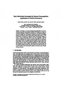
To assess the performance of the DWS system during query execution, 27 queries from the TPC Benchmark DS (TPC-DS) were run. The queries were selected based on their intrinsic characteristics and taking into account the changes needed for the queries to be supported by the PostgreSQL DBMS. Note that, as the goal is to evaluate the data distribution algorithms and not to compare the performance of the system with other systems, the subset of queries used is sufficient. The complete set of TPC-DS queries used in the experiments can be found in [2]. Data warehouse of 1Gb Figure 1 shows the results obtained for five of the TPC-DS queries. As we can see, for some queries the execution time is highly dependent on the data distribution algorithm, while for some other queries the execution time seems to be relatively independent from the data distribution algorithm used to populate each node. The execution times for all the queries used in the experiments can be found at [2]. As a first step to understand the results for each query, we analyzed the execution times of the queries in the individual nodes of the cluster. Due to space reasons we only focus on the results of queries 24 and 25. These results are listed in Table 3, along with the mean execution time and the coefficient of variation of the execution times of all nodes. By comparing the partial execution times for query 25 (see Table 3) to its overall execution time (displayed in Figure 1), it is apparent that the greater the unbalance of each node’s execution time, the longer the overall execution time of the query. The opposite, though, is observed for query 24: the distribution with the largest unbalance of the cluster nodes’ execution times is also the fastest. In fact, although in this case round-robin 10000 presents one clearly slower node, it is still faster than the slowest node for any of the other distributions, resulting in a faster overall execution time for the query. The analysis of the execution plan for query 24 showed that the steps that decisively contribute for the total execution time are three distinct index scans (of the indexes on the primary keys of dimension tables customer, customer address, and item), executed after retrieving the fact rows from table web sales that comply with a given date constraint (year 2000 and quarter of year 2). Also for query 25, the first step of the execution is retrieving the fact rows from table catalog returns that correspond to year 2001 and month 12, after which four index
8
Efficient Data Distribution for DWS
Fig. 1. Execution times for each data distribution of a 1Gb data warehouse. Table 3. Execution times in each node of the cluster (DW of 1Gb). Query Node 1 2 24 3 4 5 cv(%) 1 2 25 3 4 5 cv(%)
Random 31391 28089 38539 31288 35783 12,49% 8336 7073 12349 8882 8782 21,60%
RR1 30893 30743 35741 29704 33625 7,72% 8519 9094 11620 8428 8666 14,47%
execution times (ms) RR10 RR100 RR1000 RR10000 Hash-based 28702 24617 19761 20893 27881 29730 24812 20284 3314 27465 29296 23301 20202 3077 29500 29683 24794 23530 6533 31595 28733 27765 21144 21976 30782 1,70% 6,54% 7,19% 85,02% 6,07% 7775 7426 8293 1798 7603 8338 7794 13763 1457 7109 7523 7885 14584 6011 9022 7175 8117 2927 1533 9732 7561 7457 1881 19034 8621 5,59% 3,79% 71,22% 126,57% 12,62%
scans are executed (of the indexes on the primary keys of dimension tables customer, customer address, household demographics, and customer demographics). In both cases, the number of eligible rows (i.e., rows from the fact table that comply with the date constraint) determines the number of times each index is scanned. Table 4 depicts the number of rows in table web sales and in table catalog returns in each node, for each distribution, that correspond to the date constraints being applied for queries 24 and 25.
Efficient Data Distribution for DWS
9
Table 4. Number of facts rows that comply with the date constraints of queries 24 (table web sales) and 25 (table catalog returns). Fact table
web sales
Node 1 2 3 4 5
cv(%)
catalog returns
cv(%)
1 2 3 4 5
Random 4061 3990 4101 4042 4083 1,06% 489 475 490 468 464 2,49%
RR1 4055 4055 4056 4056 4055 0,01% 477 477 477 477 478 0,09%
# of facts rows RR10 RR100 RR1000 RR10000 Hash-based 4054 4105 3994 9529 4076 4053 4052 4283 19 3999 4055 4002 3999 7 4044 4053 4002 3998 740 4139 4062 4116 4003 9982 4019 0,09% 1,34% 3,14% 128,58% 1,35% 487 499 404 16 483 470 495 982 6 462 472 511 960 227 470 479 457 28 10 484 478 424 12 2127 487 1,40% 7,54% 100,03% 194,26% 2,24%
As we can observe, the coefficient of variation of the number of eligible facts rows in each node increases as we move from round-robin 1 to round-robin 10000, being similar for random and hash-based distributions. This is a consequence of distributing increasingly larger groups of sequential facts rows from a chronologically ordered set of data to the same node: with the increase of the round-robin “window”, more facts rows with the same value for the date key will end up in the same node, resulting in an increasingly uneven distribution (in what concerns the values for that key). In this case, whenever the query being run applies a restriction on the date, the number of eligible rows in each node will be dramatically different among the nodes for a round-robin 10000 data distribution (which results in some nodes having to do much more processing to obtain a result than others), but more balanced for random or round-robin 1 or 10 distributions. Nevertheless, this alone does not account for the results obtained. If that was the case, round-robin 10000 would be the distribution with the poorer performance for both queries 24 and 25, as there would be a significant unbalance of the workload among the nodes, resulting in a longer overall execution time. The data in Table 5 sheds some light on why this data distribution yielded a good performance for query 24, but not for query 25: it displays the average time to perform two different index scans (the index scan on the index of the primary key of the dimension table customer, executed while running query 24, and the index scan on the index of the primary key of the dimension table customer demographics, executed while running query 25) as well as the total number of distinct foreign keys (corresponding to distinct rows in the dimension table) present in the queried fact table, in each node of the system, for round-robin 1 and round-robin 10000 distributions. In both cases, the average time to perform the index scan on the index over the primary key of the dimension table in each of the nodes was very similar for round-robin 1, but quite variable for round-robin 10000. In fact, during the
10
Efficient Data Distribution for DWS
Table 5. Average time to perform an index scan on dimension table customer (query 24) and on dimension table customer demographics (query 25).
Query Algorithm Node
round-robin 1 24
round-robin 10000
round-robin 1 25
round-robin 10000
1 2 3 4 5 1 2 3 4 5 1 2 3 4 5 1 2 3 4 5
execution index scan total # of diff. time on dimension values of foreign (ms) avg time (ms) # of times perf. key in f. table 30893 3.027 4055 42475 30743 3.074 4055 42518 35741 3.696 4056 42414 29704 2.858 4056 42458 33625 3.363 4055 42419 20893 0.777 9529 12766 3314 17.000 19 12953 3077 19.370 7 12422 6533 1.596 740 12280 21976 0.725 9982 12447 8519 0.019 38 28006 9094 0.019 32 27983 11620 0.019 22 28035 8428 0.019 32 28034 8666 0.017 39 28035 1798 66.523 1 29231 1457 73.488 1 29077 6011 34.751 2 29163 1533 0 29068 19034 19.696 146 23454
execution of query 24, the index scan on the index over the primary key of the table customer was quite fast in nodes 1 and 5 for the round-robin 10000 distribution and, in spite of having the largest number of eligible rows in those nodes, they ended up executing faster than all the nodes for the round-robin 1 distribution. Although there seems to be some preparation time for the execution of an index scan, independently of the number of rows that are afterwards looked for in the index (which accounts for the higher average time for nodes 2, 3 and 4), carefully looking at the data on Table 5 allows us to conclude that the time needed to perform the index scan in the different nodes decreases when the number of distinct primary key values of the dimension that are present in the fact table scanned also decreases. This way, the relation between the number of distinct values for the foreign keys and the execution time in each node seams to be quite clear: the less distinct keys there are to look for in the indexes, the shorter is the execution time of the query in the node (mostly because the less distinct rows of the dimension that need to be looked for, the less pages need to be fetched from disk, which dramatically lowers I/O time). This explains why query 24 runs faster in a roundrobin 10000 data distribution: each node had fewer distinct values of the foreign key in the queried fact table. For query 25, as the total different values of foreign
Efficient Data Distribution for DWS
11
key in the queried fact table in each node was very similar, the predominant effect was the unbalance of eligible rows, and round-robin 10000 data distribution resulted in a poorer performance. These results ended up revealing an crucial aspect: some amount of clustering of fact tables rows, concerning each of the foreign keys, seems to result in an improvement of performance (as happened for query 24), but too much clustering, when specific filters are applied to the values of that keys, result in a decrease of performance (as happened for query 25). Data warehouse of 10Gb The same kind of results were obtained for a DWS system equivalent to a 10Gb data warehouse, and the 3 previously identified behaviours were also found: queries whose execution times do not depend on the distribution, queries that run faster on round-robin 10000, and queries that run faster on the random distribution (and consistently slower on round-robin 10000). In this case, as the amount of data was significantly higher, the random distribution caused better spreading of the data than the round-robin 10 and 100 caused in the 1Gb distribution. But even though the best distribution was not the same, the reason for it is similar: eligible rows for queries were better distributed among the nodes and lower number of distinct primary keys values of the dimension on the fact tables determined the differences.
5
Conclusion and future work
This work analyzes three data distribution algorithms for the loading of the nodes of a data warehouse using the DWS technique: random, round-robin and a hashbased algorithm. Overall, the most important aspects we were able to draw from the experiments were concerning two values: 1) the number of distinct values of a particular dimension within a queried fact table and 2) the number of rows that are retrieved after applying a particular filter in each node. As a way to understand these aspects, consider, for instance, the existence of a data warehouse with a single fact table and a single dimension, constituted by 10000 facts corresponding to 100 different dimension values (100 rows for each dimension value). Consider, also, that we have the data ordered by the dimension column and that there are 5 nodes. There are two opposing distributions possible, which distribute evenly the rows among the five nodes (resulting 2000 rows in each node): a typical round-robin 1 distribution that copies one row to each node at a time, and a simpler one that copies the first 2000 rows to the first node, the next 2000 to the second, and so on. In the first case, all 100 different dimension values end up in the fact table of each node, while, in the second case, the 2000 rows in each node have only 20 of the distinct dimension values. As consequence, a query execution on the first distribution may imply the loading of 100% of the dimension table in all of the nodes, while on the second distribution a maximum of 20% of the dimension table will have to be loaded in each node, because each node has only 20% of all the possible distinct values of the dimension.
12
Efficient Data Distribution for DWS
If the query run retrieves a large number of rows, regardless of their location on the nodes, the second distribution would result in a better performance, as fewer dimension rows would need to be read and processed in each node. On the other hand, if the query has a very restrictive filter, selecting only a few different values of the dimension, then the first distribution will yield a better execution time, because these different values will be more evenly distributed among the nodes, resulting in a more distributed processing time, thus lowering the overall execution time for the query. The aforementioned effects suggest an optimal solution to the problem of the loading of the DWS. As a first step, this loading algorithm would classify all the dimensions in the data warehouse as large dimensions and small dimensions. Exactly how this classification would be done depends on the business considered (i.e., on the queries performed) and must also account the fact that this classification might be affected by subsequent data loadings. The effective loading of the nodes must then consider complementary effects: it should minimize the number of distinct keys of any large dimension in the fact tables of each node, minimizing the disk reading on the nodes and, at the same time, it should try to split correlated rows among the nodes, avoiding that eligible rows of typical filters used in the queries end up grouped in a few of them. However, to accomplish that, it appears to be impossible to decide beforehand a specific loading strategy to use without taking the business into consideration. The suggestion here would be to analyze the types of queries and filters mostly used in order to decide what would be the best solution for each case.
References 1. Agosta, L., “Data Warehousing Lessons Learned: SMP or MPP for Data Warehousing”, DM Review Magazine, 2002. 2. Almeida, R., Vieira, M., “Selected TPC-DS queries and execution times”, http: //eden.dei.uc.pt/~mvieira/. 3. Bernardino, J., Madeira, H., “A New Technique to Speedup Queries in Data Warehousing”, Symp. on Advances in DB and Information Systems, Prague, 2001. 4. Bernardino, J., Madeira, H., “Experimental Evaluation of a New Distributed Partitioning Technique for Data Warehouses”, International Symp. on Database Engineering and Applications, IDEAS’01, Grenoble, France, 2001. 5. Bob Jenkins, “Hash Functions”, “Algorithm Alley”, Dr. Dobb’s Journal, Sep., 1997. 6. Critical Software SA, “DWS”, www.criticalsoftware.com. 7. DATAllegro, “DATAllegro v3”, www.datallegro.com. 8. ExtenDB, “ExtenDB Parallel Server for Data Warehousing”, www.extendb.com. 9. Kimball, R., Ross, M., “The Data Warehouse Toolkit: The Complete Guide to Dimensional Modeling (2nd Edition)”, Ed. J. Wiley & Sons, Inc, 2002. 10. Netezza, “The Netezza Performance Server DW Appliance”, www.netezza.com. 11. Sun Microsystems, “Data Warehousing Performance with SMP and MPP Architectures”, White Paper, 1998. 12. Transaction Processing Performance Council, TPC BenchmarkTM DS (Decision Support) Standard Specification, Draft Version 32 (2007), www.tpc.org/tpcds.