Efficient detection of zero-day Android Malware using Normalized Bernoulli Naive Bayes Luiza Sayfullina∗ , Emil Eirola† , Dmitry Komashinsky‡ , Paolo Palumbo‡ , Yoan Miche¶ , Amaury Lendasse§ and Juha Karhunen∗ ∗ Aalto University, Espoo, Finland, Email:
[email protected] † Arcada Univerity of Applied Sciences, Helsinki, Finland, Email:
[email protected] ‡ F-Secure Corporation, Helsinki, Finland, Email:
[email protected] § The University of Iowa, Iowa, USA, Email:
[email protected] ¶ Nokia Networks, Espoo, Finland, Email:
[email protected]
Abstract—According to a recent F-Secure report, 97% of mobile malware is designed for the Android platform which has a growing number of consumers. In order to protect consumers from downloading malicious applications, there should be an effective system of malware classification that can detect previously unseen viruses. In this paper, we present a scalable and highly accurate method for malware classification based on features extracted from Android application package (APK) files. We explored several techniques for tackling independence assumptions in Naive Bayes and proposed Normalized Bernoulli Naive Bayes classifier that resulted in an improved class separation and higher accuracy. We conducted a set of experiments on an up-to-date large dataset of APKs provided by F-Secure and achieved 0.1% false positive rate with overall accuracy of 91%. Keywords-Malware Classification; Naive Bayes; Security in Android;
I. I NTRODUCTION The market of Android applications continues to grow despite the fact that it is one of the most likely sources of malware among other mobile platforms. Detected malware applications are usually grouped into families that perform similar types of hazards. According to a report, provided by an F-Secure, a leading anti-virus vendor, 88% of malware families are profit-oriented [1]. In 2014 most of the detected Android malware belonged to the Trojan family. Premium SMS-sending is one of the most common malicious activities. Trojan threats also include bank frauds and data theft, that occurred in 10% of the detected malware. According to statistics provided by in Kaspersky Security Bulletin 2014 [2], 4,643,582 malicious Android installation packages were detected during the period from November 2013 to the end of October 2014. Out of them, 12,100 were mobile banking Trojans. 19% of Android users of Kaspersky products encountered a threat at least once during the year. Similarly to the F-Secure report, the most common threat was Trojan-SMS.AndroidOS.Stealer.a that occurred in 18% of the threats along with other SMS-sending Trojans.
Despite the fact that new malware types and variations are created, they can be efficiently classified as malicious due to similarities with existing malware. In this paper we present in detail an improved Naive Bayes classifier [3], [4] to detect malicious Android applications based only on the features from APKs. It is highly important to have a low false malicious rate not to block users from downloading clean software and not to irritate customers much with security alerts. In addition blocking clean applications can lead to revenue loss of the application owner. At the same time we should try to keep a low false benign rate to provide high level of security. We refer to a malicious class as to a positive class, so true malicious rate means true positive rate (TPR), true benign rate means true negative rate (TNR), false malicious and false benign rates are FPR and FNR respectively. In our paper, we focus on achieving low FPR. In Section II, we describe the content of APK files and what features were used from those files for classification. Section III is dedicated to outlining the existing approaches for tackling Naive Bayes independence assumptions and presenting the experimental results on our dataset. In the next section, we introduce Normalized Bernoulli Naive Bayes, that outperforms Bernoulli Naive Bayes with lower FPR and better classification boundary. In Section V, we make an overview of recent publications in Android malware classification and state our contribution to existing work in this area. II. DATA D ESCRIPTION In the proposed approach we make a static analysis of the application through its APK installation package. Now we briefly explain the structure of an APK package and the groups of features we extracted. Every Android installation package has three main files: AndroidManifest.xml, classes.dex and resources.arsc. First file AndroidManifest.xml [17] contains general information about the application to be installed. It provides the summary of the resources, permissions needed to run the application and
File
Groups of features
AndroidManifest.xml
entries, packages, permissions, strings
classes.dex
classes, fields, methods, prototypes, types, strings
resources.arsc
strings
other files
hashes, names
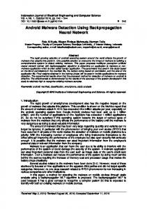
Table I: Features selected from APK files Figure 1: The histogram of APK file sizes, totally 120,000 files.
its components, including services, activities, libraries, entry points, their capabilities, etc. All the elements in AndroidManifest.xml file, except and are optional. Practically this means that one should expect diversity of features across files. If a fixed set of features is used, we should be sure that those are highly representative features of malware and that they can be found at least in malware APKs. However, this cannot be always guaranteed due to the diversity of malware families. In addition, while aiming at high performance and reliability, we use a large set of features, but still apply feature selection heuristics to reduce the number of features and to omit irrelevant ones. The second obligatory file classes.dex contains compiled Java byte-code of the application. Data from classes.dex header gives us the opportunity to extract the arrays of strings. These strings include parts of the Java code, specifically classes, methods, types, etc. Hence the analysis of Java code is partially performed as well. The third file resources.arsc consists of precompiled resources in a binary format. It may include images, icons, strings, or other data used by the application. DEX (Dalvik Executable) [18] is a file format that contains compiled code written for Android and can be interpreted by the Dalvik virtual machine. DEX files can be created manually or by automatically translating compiled Java programs. Multiple DEX files are zipped into a single APK, which serves as the final Android application file. Files from res, META-INF folders and root folders are described only by their names and hashes. At the same time, items from AndroidManifest.xml, resources.arsc and classes.dex are used as features more extensively. In Table I we list what entries from APK files are taken as features for the classifier. Data for the experiments was provided by F-Secure. We have more than 120,000 files with trustworthy information about the class (benign or malicious) from 2014. The histogram of file sizes is shown in Figure 1. We can observe that larger files are less likely to be malicious. Besides that, there is a huge number of small files, less than 1000 Kb, most of
which are malicious. So both the file sizes and the feature set sizes show large variation. In the following subsection, we proceed with the explanation of the Naive Bayes Classifier and its existing modifications. III. NAIVE BAYES C LASSIFIER AND ITS EXISTING MODIFICATIONS
The Naive Bayes Classifier (NB) has been applied in diverse fields, especially in language processing and bioinformatics, including text genre classification and authorship attribution [19], sentiment analysis [20], predicting diseases from genome data [21]. The classifier is called “naive”, as it assumes that all features are independent, conditional on the class label. Then the class conditional densities can be presented as follows: p(w|c, φ) =
D Y
p(wi |c, φic ) ,
(1)
i=1
where D is the dimension of the feature vector w = (w1 , w2 , ..., wD ), φic ∈ φ is a maximum-likelihood estimate of the feature wi for a class c. Features extracted from APK packages are very likely to be dependent, at least, the Java code features. We elaborate on how to tackle naive independence assumptions in the next section. Malware classification, as text classification, involves high-dimensional samples. However, unlike in text, features taken from APKs are not restricted to some small vocabulary, but rather consist of code strings, various languages, hashes, names and other meta information. The number of features in our problem is larger than in most languages due to the presence of different spoken languages, programming language strings, hashes, etc. Some of these features are most likely independent, some of them are irrelevant for the classification. Moreover, due to diversity of file sizes, there is a big spread in the amount of available features for each file. In the next section we aim to show already existing approaches in text classification to tackle independence assumptions and different number of features across the files. A. Bernoulli Naive Bayes A Bernoulli NB model was chosen due to the relevance of using binary features in a two class classification problem.
This is because most of the features occur only once and malware can most probably be characterized by the presence of a feature, rather than its quantity. In Bernoulli setting the class conditional density is as follows: p(w|y = c, φ) =
=
D Y i=1 D Y
Ber(wi |φic ) (2) 1−wi i , φw ic (1 − φic )
i=1
where y is the output vector with class labels for N files. The classification problem in our context is to predict whether the file is malicious or benign, so c = {mal, ben}. File is represented by a binary vector w = (w1 , w2 , ..., wD ), where wi = 1 if the ith feature present in the file. At the same time we can estimate likelihood without modeling absence terms: p(w|y = c, φ) =
D Y
i φw ic
(3)
i=1
Modeling term absence in high dimensional feature space is not always practical or beneficial. One of the reasons is that the absence probability estimate 1 − φic can dominate significantly over the low presence probability estimate φic for most of the features. It can occur due to extremely sparse dataset. We present in section B the experiments on modeling the absence features and show that they reduce the quality of the Bernoulli NB for our problem. Now we present the posterior as a ratio of the probability of a file to belong to a malicious class to the probability of belonging to a benign class. This formula takes into account only present features and can be found in [22]. So, in order to determine a class for a file f , we need to evaluate the following formula: F p(mal) Y p(wi = 1|mal) p(y = mal|f ) = · , p(y = ben|f ) p(ben) i=1 p(wi = 1|ben)
(4)
where F denotes the number of features in the file f that intersect with the training set features. We change the formulas to log scale to avoid arithmetic overflow and for better interpretation. The Naive Bayes rule can be reformulated using log-likelihood ratios as follows: θi = log
p(wi = 1|mal) p(wi = 1|ben)
(5)
and the posterior ratios as: log
F X
p(y = mal|f ) p(mal) = log + θi . p(y = ben|f ) p(ben) i=1
(6)
In log scale a positive ratio shows that a feature occurs more in the malicious class than benign.
B. Existing techniques for tackling independence assumptions Despite the fact that in [26] the authors show that NB classifiers can result in near optimal accuracy with the independence assumptions, there has been much work to tackle this assumption. In [27], several weight modification methods were proposed to tackle independence assumption and to mimic language distribution in Multinomial NB. The proposed techniques included normalizing maximum loglikelihood estimates θic for the ith feature in a class c ∈ C by the sum of log estimates of all features, that is: θci . θic = P k θck
(7)
Another modification from [27] is multiplying the frequency of the ith word in the j th document dij by the Inverse Document Frequency [28], driven from Information Retrieval: P 1 (8) dij = dij P k , k δik th th where Pδij is 1, if the i word occurs in the j document and k 1 is the number of documents. The authors in [27] also proposed to normalize the ith feature frequency by the total sum of frequencies of words in the j th document:
dij dij = qP k
.
(9)
d2kj
In our binary vector setting this formula is equivalent to document length normalization. Taking into account the diversity of file sizes, normalization changes the term frequencies differently across the files. These three ideas were tested, but they did not increase the performance of both Bernoulli NB and Multinomial NB classifiers. We provide the results of our experiments in Table II. A dataset for this and later experiments contains 10,000 samples in the training set and 10,000 in test set with equal number of malicious and benign files in both sets. Laplace smoothing parameter k is set to 0.0001 (we show why in Section IV D) and only the features, that were seen more than two times in the training phase were taken into account for classification. From Table II we can infer, that Multinomial NB does not bring any good results for our binary features. IV. I MPROVED IMPLEMENTATION OF B ERNOULLI NAIVE BAYES The results of this section are based on the techniques that we introduced for Bernoulli Naive Bayes in order to achieve low FPR and keep reasonably good TPR. These modifications include: simple, but effective feature selection, scaling, tuned Laplace smoothing and decision boundary selection.
method
modification
FPR, %
TPR, %
Settings
FPR, %
TPR, %
# features
Bern.
standard
0.08
67.42
α = 3, β = 3
0.46
82.9
4833680
Bern.
Eq. 7
0
0.18
α = 3, β = 4
0.46
83.00
4818990
Bern.
Eq. 8
0.08
69.88
α = 3, β = 5
0.46
83.12
4786793
Bern.
Eq. 9
0.04
60.36
α = 4, β = 3
0.46
80.76
3710978
Bern.
no absent, Eq. 7
0
0.26
α = 4, β = 4
0.42
80.78
3698627
Bern.
no absent, Eq.8
0.08
68.82
Bern.
no absent, Eq. 9
0.04
60.36
Multin.
standard
0.02
30.14
Multin.
Eq. 7
0
0.18
Multin.
Eq. 8
0.04
27.20
Multin.
Eq. 9
0.04
41.36
Bern.
no absent, scaling
0.10
82.10
Table II: Experiments with Bernoulli and Multinomial NB with modifications. “no absent” denotes ignoring absence features. From the last line of the table we can infer that proposed Normalized Bernoulli NB outperforms other modifications with 99.9% TNR and 82.1% TPR.
A. Feature Selection Despite the fact that NB is a scalable algorithm, we would like to optimize the complexity and discard potentially irrelevant features. We decided to restrict the minimum occurrence for each feature, denoted as α and minimum number of letters in the feature as β. We found that to keep high accuracy even features seen in 3 files were beneficial. To control the number of features, we filter them by β. By random selection of short features we figured out that short strings denoted numbers and other random strings unrelated to the code. The results of experiments with different thresholds are shown in Table III. By setting the threshold α = 3, we have a wider set of features and a better accuracy. The performance did not decrease much by setting a higher β, but we benefited from discarding noninformative features. As stated in [29], omitting infrequent features is not the best strategy in this classifier. B. Scaling Now we present our own modifications, based on normalizing the sum of log-factors during classification. In Equation 6 the number of log-factors θi to sum up is different for each file. So while summing log-factors θi for each file f during the classification, the size of the file can introduce potential bias to the sum. Indeed we are using a different number of features in the sum and some normalization is needed to compare the sum across the files. In order to decrease the bias, the sum of factors is divided
Table III: The effect of different settings in feature selection on the performance of Normalized NB. α denotes a threshold of the minimum feature occurrence and β denotes the minimum number of letters in the feature name.
by the number of features with non-zero θi equal to F : D(f ) =
F 1 X θi . F i=1
(10)
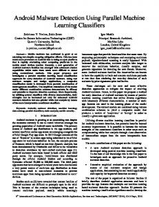
We call this modification Normalized Bernoulli NB. Next we illustrate the effect of using modified log-likelihood on the decision boundary. As the final decision depends on log-factor sums, the analysis of their histogram gives a good intuition about how successful we are in achieving the best possible FPR. Now we compare the boundaries of standard and Normalized Bernoulli NB in their classification performance. The experimental balanced dataset as before contains 20,000 samples from both classes, k = 0.0001, α = 3 and β = 5. The values of α and β were chosen based on the results of previous feature selection experiments. In Figures 2 and 3 the histograms of log-factor sums for both methods are shown. In Bernoulli NB the boundary between two classes is asymmetrical and a low FPR is achieved easier than a low FNR. By achieving a low FPR, we get a relatively high FNR. Moreover, I performed a separate experiment with cross-validation, where 20,000 samples were divided into 4 folds and each time 2 folds served as a training set and 2 folds as a testing set. Average FPR of 0.067% and TPR of 87.338% were achieved. Next, compare Figure 2 and Figure 3 which shows Normalized Bernoulli NB for the value of k = 0.0001. The intersection of false malicious and false benign logfactor sums is more symmetric in Figure 3. In addition to that, low FPR can be achieved with lower FNR. Thus, modified method proves to be more effective for the current problem in achieving both low FPR and FNR. Complexity stays linear, however to find the border to achieve low FPR takes additional pass through zero-class instances from training set. We will explain how to select the decision boundary in advance to achieve the desired low FPR in the following section. At the same time adjusting k may take several validation experiments. We make as well remarks on
Figure 2: The histogram of log-factor sums D(f) for malicious and benign test files using Bernoulli NB. The intersection between two histograms is quite skewed. It is more difficult to find the border to get desired FNR due to the heavy-tail distribution of the intersection between two classes.
Figure 3: The histogram of log-factor sums D(f) for malicious and benign test files using Normalized Bernoulli NB. The boundary in this case is more clear. We can adjust the boundary to get low FPR or FNR. The histogram does not have a heavy-tail in the intersection between two classes unlike in standard Bernoulli NB.
choosing parameter k to have better class separation. C. Selecting the decision boundary A natural question that arises when assigning the class label is how the class boundary between two classes is decided. As we use factors θi in a log scale, the default
boundary for sum D(f ) from Equation 10 would be zero. However, taking into account our low FPR preference, we try to find such a boundary that we achieve close to 0 FPR. In this section we show also why our proposed Normalized Bernoulli NB is a better method compared to Bernoulli NB for selecting the boundary between the classes.
The boundary is selected using D(f ) while calculating log-factors θi ∈ θ. In order to make low FPR, we have chosen the max D(f ) for benign files. It is the value of the classification boundary, where the highest TPR is achieved with FPR = 0. For example in Figure 3 the boundary in the test set would be the point belonging to the right most green bar. k
FPR, %
TPR, %
1
0.08
43.16
0.1
0.08
62.78
0.01
0.18
75.0
0.001
0.32
80.04
0.0001
0.42
83.14
Table IV: The effect of parameter k on classification performance in the test set.
D. Tuning Laplace smoothing parameter It has been shown in [23] that by smoothing maximum likelihood estimate as well as log-factors θi we avoid zero probabilities for some features. In Laplace smoothing [23] it is implemented by adding small constant k to both the number of malicious files with feature wi denoted as c(wi , mal) and to the number of benign files with feature wi as c(wi , ben): θi = log
c(wi ,mal)+k M +2k c(wi ,ben)+k B+2k
,
(11)
where B and M are the numbers of malicious and benign files accordingly. In [24], k is chosen to be 1; however in [25] k is proposed to be N1 , where N is the number of training samples. We conducted an experiment on the same balanced dataset with α = 3, β = 5 and several values of k, using Normalized Bernoulli NB. The purpose of the experiment was to compare overall performance and to see how low FPR we can achieve. It is clearly seen from Table IV, that with increasing k the performance drops. However, at the same time with increasing k FPR decreases. Although with k = 1 TPR does not seem to be trustworthy. This experiment agrees with the proposition of [25] to set k = N1 . V. OVERVIEW OF THE STATE OF THE ART Malware classification methods fall into two main categories: dynamic and static. First one implies performing dynamic analysis, where malicious behavior is detected after a sample is executed in the experimental environment or via sandboxing. An elaborated survey on dynamic malwareanalysis techniques is presented in [5]. The scope of our
method is based on a static off-device approach, so we focus on the overview of the static approaches here. Static-based methods can be classified into signaturebased and machine learning-based. In this approach an application is analyzed without being executed, but based on its features. Signature-based features are less reliable as they can be obfuscated by bytecode-level code transformation [6]. Another type of features can be extracted from APK package files or by decompilation of APK files to Java code. Extracted features have been used for malware classification in several areas, including Data Mining [7], Machine Learning [8], Clustering [9], etc. Graph representations are widely used for code analysis. Android malware classification using features from a Java code of the APKs was implemented in [6]. In this paper, Java byte-code is transformed into a corresponding graph representation. The similarity of the features is measured by the similarity of the corresponding graphs which enable better understanding of API calling contexts. In [10] two-level behavioral graph representation is used to capture Android application logic and to label elements of the graph that capture malicious behavioral patterns. The authors predict most probable malware family and find malicious modalities. Malicious applications were identified with 95.3% detection rate and only 0.4% FPR. Machine Learning techniques, including Support-vector machines (SVM) [11], Naive Bayes combined with feature selection are popular as well, however they differ a lot in the feature engineering approaches. We want to outline the results of [12] and [8] whose papers are closely related to our work. In [12], only permissions from AndroidManifest.xml files are used in a One-Class-SVM classifier with kernels. Authors solely use benign application samples and permissions out of the diverse set of features that can potentially be mined from APK data. Another related paper is [8], where a Naive Bayes Classifier is used for analysis of reversed-engineered APK Java code. After getting Java code from compiled files, a Java-code analyzer mines a set of features, including API calls, commands, permissions, etc. Top 25 features selected by Mutual Information [13] are used in Naive Bayes classifier. On a small test set with 1000 samples, the classification accuracy reaches 92.1%, FPR is 6.3% and TPR is 90.6%. One of the weakness in the paper is that FPR is quite high. Selecting only 25 features might be insufficient for generalizing to new unseen samples due to the variety of malware families. In [14], features from APK files were used to classify Android applications into two categories: games and tools due to unavailability of malicious and benign files. However, they evaluated several Machine Learning methods, including Decision Tree [15], Naive Bayes, Boosted Bayesian Networks [16] and etc. Boosted Bayesian Networks with 800 features selected by Information Gain yielded 17.2% FPR and accuracy of 91.8%.
The main contribution of our paper in the group of static approaches is its low complexity and the ability to achieve low FPR in comparison to the existing methods. The classification boundary of the Naive Bayes classifier can be adjusted to get the desired balance between FPR and TPR. Using our Normalized Bernoulli NB, we can achieve FPR = 5% and TPR = 98% or even lower FPR = 0.1% with TPR = 82.1% outperforming the above-mentioned state of the art results. Compared to mentioned Machine Learning techniques, we prefer soft feature selection instead of a tight one to generalize better to new unseen samples. In addition, Normalized Bernoulli NB can be implemented in Java and installed on the mobile phone to classify new applications to be installed.
[4] K. P. Murphy, Machine Learning A Probabilistic Perspective. The MIT Press, 2012. [5] M. Egele, T. Scholte, E. Kirda, and C. Kruegel, “A survey on automated dynamic malware-analysis techniques and tools,” ACM Computing Surveys (CSUR), vol. 44, no. 2, p. 6, 2012. [6] M. Zhang, Y. Duan, H. Yin, and Z. Zhao, “Semantics-Aware Android malware classification using weighted contextual API dependency graphs,” in Proceedings of the 2014 ACM SIGSAC Conference on Computer and Communications Security, ser. CCS ’14. ACM, 2014, pp. 1105–1116. [7] G. Suarez-Tangil, J. E. Tapiador, P. Peris-Lopez, and J. Blasco, “Dendroid: A text mining approach to analyzing and classifying code structures in android malware families,” Expert Systems with Applications, vol. 41, no. 4, Part 1, pp. 1104 – 1117, 2014.
VI. C ONCLUSION [8] S. Yerima, S. Sezer, G. McWilliams, and I. Muttik, “A new Android malware detection approach using Bayesian classification,” in 2013 IEEE 27th International Conference on Advanced Information Networking and Applications (AINA), March 2013, pp. 121–128.
In this paper we introduced the static algorithm for Android Malware Classification that keeps low FPR, high overall accuracy and performs real-time classification. The features from Android application package files, including AndroidManifest.xml, classes.dex and resources.arsc were used for classification. We presented Normalized Bernoulli NB, that outperforms Bernoulli NB and some of its existing modifications in the accuracy and gives a better class separation. Our modification involves tuning Laplace smoothing parameter and normalizing the sum of log-factors by the length of the file. Using Normalized Bernoulli NB we achieved very low FPR of 0.1% and TPR of 82.10% with 10,000 training and 10,000 test samples. As a result our fast and easy-implementable approach can be used by antivirus companies to protect their Android users. The decision making algorithm can be implemented on an Android mobile phone in Java. The approach presented in this paper is currently being expanded by F-Secure.
[10] C. Yang, Z. Xu, G. Gu, V. Yegneswaran, and P. Porras, “Droidminer: Automated mining and characterization of finegrained malicious behaviors in android applications,” in Computer Security - ESORICS 2014, ser. Lecture Notes in Computer Science, 2014, vol. 8712, pp. 163–182.
VII. ACKNOWLEDGEMENTS *
[13] T. M. Cover and J. A. Thomas, Elements of Information Theory. New York, NY, USA: Wiley-Interscience, 1991.
This work was supported by the Academy of Finland ”Cloud Security Services” project (13283212). Special thanks to Professor N. Asokan from Aalto University and senior researcher Alexey Kirichenko from F-Secure for giving precious comments about the paper. R EFERENCES [1] F-Secure, “Mobile threat report q1 2014.” [Online]. Available: https://www.f-secure.com/documents/996508/1030743/ Mobile Threat Report Q1 2014.pdf [2] M. Garnaeva, V. Chebyshev, D. Makrushin, R. Unuchek, and A. Ivanov, “Kaspersky security bulletin 2014. Overall statistics for 2014.” [Online]. Available: http: //securelist.com/analysis/kaspersky-security-bulletin/68010/ kaspersky-security-bulletin-2014-overall-statistics-for-2014/ [3] D. Barber, Bayesian Reasoning and Machine Learning. Cambridge University Press, 2012.
[9] E. Gandotra, “Malware analysis and classification: A survey,” Journal of Information Security, no. 5, pp. 56–64, 2014.
[11] C. Cortes and V. Vapnik, “Support-vector networks,” Machine Learning, vol. 20, no. 3, pp. 273–297, 1995. [12] J. Sahs and L. Khan, “A machine learning approach to Android malware detection,” in European Intelligence and Security Informatics Conference (EISIC), Aug 2012, pp. 141– 147.
[14] A. Shabtai, Y. Fledel, and Y. Elovici, “Automated static code analysis for classifying android applications using machine learning,” in Computational Intelligence and Security (CIS), 2010 International Conference on, 2010, pp. 329–333. [15] J. R. Quinlan, “Induction of decision trees,” Machine Learning, vol. 1, no. 1, pp. 81–106, Mar. 1986. [16] Y. Jing, V. Pavlovi´c, and J. M. Rehg, “Boosted bayesian network classifiers,” Machine Learning, vol. 73, no. 2, pp. 155–184, 2008. [17] “App manifest.” [Online]. Available: http://developer.android. com/guide/topics/manifest/manifest-intro.html [18] “Dalvik executable format.” [Online]. Available: http: //source.android.com/devices/tech/dalvik/dex-format.html [19] F. Peng, D. Schuurmans, and S. Wang, “Augmenting Naive Bayes classifiers with statistical language models,” Information Retrieval, vol. 7, no. 3-4, pp. 317–345, 2004.
[20] V. Narayanan, I. Arora, and A. Bhatia, “Fast and accurate sentiment classification using an enhanced Naive Bayes model,” Intelligent Data Engineering and Automated Learning IDEAL 2013, pp. 194–201, 2013. [21] W. Wei, S. Visweswaran, and G. F. Cooper, “The application of naive Bayes model averaging to predict Alzheimer’s disease from genome-wide data,” Journal of the American Medical Informatics Assosiation, pp. 370–375, 2011. [22] A. Y. Ng and M. I. Jordan, “On Discriminative vs. Generative Classifiers: A comparison of logistic regression and naive Bayes,” in Advances in Neural Information Processing Systems 14. MIT Press, 2002, pp. 841–848. [23] C. Zhai and J. Lafferty, “A study of smoothing methods for language models applied to information retrieval,” ACM Transactions on Information Systems, vol. 22, no. 2, pp. 179– 214, 2004. [24] Q. Yuan, G. Cong, and N. M. Thalmann, “Enhancing Naive Bayes with various smoothing methods for short text classification,” in Proceedings of the 21st International Conference Companion on World Wide Web, 2012, pp. 645–646. [25] R. Kohavi, B. Becker, and D. Sommerfield, “Improving simple Bayes,” 1997, Poster, presented at European Conference on Machine Learning. [26] D. P and P. M, “On the optimality of the simple Bayesian classifier under zero-one loss,” Machine Learning - Special issue on learning with probabilistic representations, vol. 29, pp. 103–130, 1997. [27] J. D. M. Rennie, L. Shih, J. Teevan, and D. R. Karger, “Tackling the poor assumptions of Naive Bayes text classifiers,” in In Proceedings of the Twentieth International Conference on Machine Learning, 2003, pp. 616–623. [28] C. D. Manning, P. Raghavan, and H. Sch¨utze, Introduction to Information Retrieval, 2008. [29] S. N. Pages and A. Aizawa, “Akiko aizawa linguistic techniques to improve the performance of automatic text categorization,” in Proceedings 6th NLP Pacific Rim Symposium NLPRS-01, 2001, pp. 307–314.