Efficient Elliptic Curve Cryptography Implementation over GF(2m)

TinyECCK: Efficient Elliptic Curve Cryptography Implementation over GF (2m ) on 8-bit MICAz Mote Seog Chung Seo1 , Dong-Guk Han2 , Seokhie Hong1 Graduate School of Information Management and Security, Korea University, {seosc, hsh}@cist.korea.ac.kr1 Electronics and Telecommunications Research Institute, [email protected]

Abstract. In this paper, we revisit a generally accepted opinion: implementing Elliptic Curve Cryptosystem (ECC) over GF (2m ) on sensor motes using small word size is not appropriate because XOR multiplication over GF (2m ) is not efficiently supported by current low-powered microprocessors. Although there are some implementations over GF (2m ) on sensor motes, their performances are not satisfactory enough to be used for wireless sensor networks (WSNs). We have found that a field multiplication over GF (2m ) are involved in a number of redundant memory accesses and its inefficiency is originated from this problem. Moreover, the field reduction process also requires many redundant memory accesses. Therefore, we propose some techniques for reducing unnecessary memory accesses. With the proposed strategies, the running time of field multiplication and reduction over GF (2163 ) can be decreased by 21.1% and 24.7%, respectively. These savings noticeably decrease execution times spent in Elliptic Curve Digital Signature Algorithm (ECDSA) operations (signing and verification) by around 15% ∼ 19%. We present TinyECCK (Tiny Elliptic Curve Cryptosystem with Koblitz curve – a kind of TinyOS package supporting elliptic curve operations) which is the fastest ECC implementation over GF (2m ) on 8-bit sensor motes using ATmega128L as far as we know. Through comparisons with existing software implementations of ECC built in C or hybrid of C and inline assembly on sensor motes, we show that TinyECCK outperforms them in terms of running time, code size and supporting services. Furthermore, we show that a field multiplication over GF (2m ) can be faster than that over GF (p) on 8-bit ATmega128L processor by comparing TinyECCK with TinyECC, a well-known ECC implementation over GF (p). TinyECCK with sect163k1 can compute a scalar multiplication within 1.14 secs on a MICAz mote at the expense of 5,592-byte of ROM and 618-byte of RAM. Furthermore, it can also generate a signature and verify it in 1.37 and 2.32 secs with 13,748-byte of ROM and 1,004-byte of RAM.

2

1

Seog Chung Seo et al.

Introduction

Many researchers have tried to apply the public-key cryptosystem, especially ECC to wireless sensor networks to overcome the limitations of the symmetrickey based protocols at pairwise key setup and broadcast authentication phases. They concluded that employing ECC is viable in WSNs: Their implementations have been shown reasonable performances in running time and code size [1, 8, 10, 15]. Until now, implementations giving relatively satisfactory performance are all based on GF (p) [1, 8, 15]. On the other hand, the implementations over GF (2m ) result in disappointing performance [4, 7, 9, 10]. Some literatures [1, 8, 10, 15] imputed the poor performances to insufficient support of field arithmetic operations over GF (2m ), especially field multiplication, of current low-powered microprocessors that work in small word size, thus the implementation of ECC over GF (2m ) would lead to lower performances. This paper revisits this opinion and shows that the field multiplication in GF (2m ) can be faster than that in GF (p). There are following misunderstandings about the implementation of ECC over GF (2m ) on sensor motes: Inefficient field multiplication: The field multiplication which is one of the most frequent operations in the elliptic curve operation in GF (2m ) is regarded as being less efficient than that in GF (p) on low-powered and small word-sized devices since it requires partial XOR multiplications which are not efficiently supported by current microprocessors at instruction level.1 Heavy memory requirement for ECDSA: ECDSA implementations over GF (2m ) require not only field arithmetic over GF (2m ) but also field arithmetic over GF (p) for generating and verifying digital signatures. Thus, it may be thought that the code size of ECDSA over GF (2m ) is larger than that over GF (p). Actually, most of existing works over GF (2m ) only implement Elliptic Curve DiffieHellman (ECDH) protocol in their motes. However, the code size of optimized implementation of ECDSA over GF (2m ) is comparable to that over GF (p). Our implementation, TinyECCK, achieves optimized code size for ECDSA and outperforms TinyECC known as the most efficient software implementation of ECDSA over GF (p) on sensor motes. The contributions of this paper are described as follows. 1. Showing field multiplication over GF (2m ) can be faster than that over GF (p): We have found that the field multiplication and reduction over GF (2m ) are involved in many redundant memory accesses. In fact, most of the intermediate results of consecutive XOR multiplications during a field multiplication over GF (2m ) are stored at the same memory destination and same values are loaded several times. We present some techniques to eliminate much of redundant memory accesses at field multiplication and reduction phases. As the result of applying the proposed techniques, the execution times of field multiplication and reduction over GF (2163 ) are saved as much as 21.1% and 1

Partial XOR multiplication: The XOR operations of partial products in the field multiplication over GF (2m ). There is no carries in XOR multiplications.

TinyECCK

3

24.7%, respectively. At this time, the running time of the proposed multiplication method is faster than the optimized field multiplication over GF (p) by 7.4%. 2. Fastest software implementation of ECC over GF (2m ): TinyECCK outperforms existing all software implementations of ECC over GF (2m ). Furthermore, TinyECCK is the fastest among the software implementations built in C or mixture of C and inline assembly over both GF (p) and GF (2m ) on ATmega128L processors. 3. Efficient implementation of Koblitz curve over GF (2m ) on 8-bit ATmega128L processor : TinyECCK implements elliptic curve operations on Koblitz curve for fast scalar multiplications. Because the point doubling operation in the Koblitz curve can be replaced by some trivial field squarings, the performance can be much improved compared with ordinary curves over GF (2m ).

2

Related Work

There have been several implementations of ECC over both GF (2m ) and GF (p) on sensor motes. They have tried to prove the feasibility of ECC for WSNs. 2.1

Existing Implementations over GF (2m )

Malan et al. implemented EccM which was the first implementation of ECC over GF (2m ) on a 8-bit sensor mote [4]. They used ECC to provide a key distribution mechanism for UC Berkeley’s TinySec [2] module. EccM takes 34 secs for generating a public key and requires 34,342-byte of ROM as code size. In [9], Yan and Shi indicated that the software implementations of ECC over GF (2m ) were still slow on small computing devices such as sensor nodes. They implemented 163-bit ECC using fast modular reduction on a 8-bit ATmega128L processor. Their implementation requires 11,592-byte of code size and takes 13.9 secs for a scalar multiplication. Eberle et al. pointed out that field arithmetic over GF (2m ), especially field multiplication is prohibitively slow since general-purpose microprocessors do not support arithmetic in that field [10]. They claimed that the performance of ECC implementation over GF (2m ) can be faster than that over GF (p) with additional architectural extension using instruction set extension. Actually, the implementation using architectural extension took only 0.29 secs for a 163-bit ECC point multiplication over GF (2m ) while their assembly implementation takes 4.14 secs. This result supports that ECC over GF (2m ) is more suitable for hardware implementation rather than software implementation. Blaß and Zitterbart implemented ECDH, ECDSA and El-Gamal over GF (2113 ) and compared their performances with those of EccM [7]. Their implementation took 6.88 and 24.17 secs for signature generation and verification, respectively. Their code occupies 75,088-byte of ROM. 2.2

Existing Implementations over GF (p)

To prove the feasibility of public-key cryptography on WSNs, Gura et al. implemented RSA and ECC over GF (p) with assembly code and instruction set

4

Seog Chung Seo et al.

extension on a 8-bit ATmega128 processor and compared the performance between RSA and ECC [15]. Their ECC implementation took only 0.81 secs for a scalar multiplication, which supports the assertion that the use of public-key cryptography, especially ECC is viable for WSNs. They also presented a hybrid multiplication algorithm exploiting advantages of operand and product scanning multiplication algorithm to reduce the number of memory accesses. TinyECC [1] is a software package providing ECC operations such as a scalar multiplication, and ECDSA services over GF (p) on TinyOS [16]. TinyECC adopted several optimization techniques such as optimized modular reduction using pseudoMersenne prime, sliding window method, Jacobian coordinate systems, inline assembly and hybrid multiplication to achieve computational efficiency. TinyECC – its major operations such as field multiplication and modular reduction are built in inline assembly – can generate a signature and verify it within 2.00 and 2.43 secs, respectively, at the cost of more code size: i.e., 19,308-byte of ROM. On the other hand, TinyECC sorely built in C takes 6.26 and 7.92 secs for generation and verification of a signature with smaller code size: i.e., 15,872-byte of ROM. Until now, the performance of ECC implementations over GF (p) surpasses those over GF (2m ) with 8-bit word. From these observations, it appears that software implementation of ECC over GF (p) outperforms that of ECC over GF (2m ) on small devices and ECC implementation over GF (2m ) is suitable only for hardware implementation. However, in this paper we show that the performance of the optimized software implementation (TinyECCK) of ECC over GF (2m ) can surpass that of the optimized one (TinyECC) of ECC over GF (p) on 8-bit sensor motes.

3

Overview of Elliptic Curve Cryptosystem

The set of solutions of following weierstrass equation over a field F forms an abelian group with the point at infinity O as its identity. E/F : y 2 + a1 xy + a3 y = x3 + a2 x2 + a4 x + a6 , ai ∈ F

(1)

In case characteristics of F is 2, the equation is simplified as follows: E/GF (2m ) : y 2 + xy = x3 + ax2 + b, a, b ∈ GF (2m )

(2)

According to the principle of abelian group, a point P3 which is result of adding two points P1 and P2 on a curve is also on the curve. Adding two different points and two same points are called elliptic curve point addition (ECADD) and elliptic curve point doubling (ECDBL). Let us assume two arbitrary points P1 = (x1 , y1 ) and P2 = (x2 , y2 ) ∈ E(GF (2m )) with P1 6= −P2 . Then the coordinate of P3 = (x3 , y3 ) which is the result of P1 + P2 can be computed as follows in affine coordinate: x3 = λ2 + λ + x1 + x2 + a, y3 = (x1 + x3 )λ + x3 + y1 , (y1 +y2 ) λ = (x if P1 6= P2 , and λ = xy11 + x1 if P1 = P2 1 +x2 )

TinyECCK

5

Both ECADD and ECDBL in affine coordinate require 1 field inversion and 2 field multiplications. It brings advantages to use projective coordinate when the field inversion is more expensive than field multiplication. For example, L´opezDahab (LD) projective coordinate requires 14 field multiplications and 4 field multiplications in ECADD and ECDBL, respectively.2 Therefore, it is expected that the use of LD coordinate is more suitable than that of affine coordinate when I > 7M (I = field inversion, M = field multiplication) on the target platform. Adding a point P to itself k times is called scalar multiplication; it is expressed as Q = kP , where k is an integer and P ∈ E(GF (2m )). This scalar multiplication is the dominant operation in ECC such as ECDH and ECDSA.

4

Implementation Details

We have implemented TinyECCK on a MICAz [14] sensor mote including the 8-bit ATmega128L processor. We use the domain parameter (sect163k1) recommended by [3] and polynomial basis to represent elements in GF (2m ). We modified the original field arithmetic algorithms using 32-bit word size which are presented in Guide to Elliptic Curve Cryptography [5, 6] into the forms suitable for 8-bit word environment. For efficiency, TinyECCK makes use of recoding algorithms such as wNAF and wTNAF and selects mixed coordinate system rather than affine coordinate. 4.1

Preliminaries

We assume that the used word size is 8-bit since the ATmega128L processor works with 8-bit word memory address. The following notations are used in the rest of this paper. Let us assume A and B are elements in GF (2m ). A ⊕ B: bitwise exclusive-or. A & B: bitwise AND. A À i: right shift of A by i positions with padding i upper bits as 0. A ¿ i: left shift of A by i positions with padding i lower bits as 0. W : a 8-bit word. U (W ): it returns (W À 4). L(W ): it returns (W & 0x0F ). A[j] denotes j-th word of the A polynomial. A{j} denotes the partial array from the most significant word (n) to j-th word (A[n], . . . , A[j + 1], A[j]). A{j, . . . , i} denotes the part of A polynomial from i-th word to j-th word (A[j], . . . , A[i + 1], A[i]), j ≥ i. t = dm/W e is the required number of words to store A in memory.

4.2

Field Arithmetic over GF (2m )

Field Squaring Squaring an element a(z) = am−1 z m−1 +. . .+a2 z 2 +a1 z +a0 in GF (2m ) results in a(z)2 = am−1 z 2m−2 + . . . + a2 z 4 + a1 z 2 + a0 that comes out by 2

Detail about L´ opez-Dahab projective coordinate can be found in [5, 6, 12].

6

Seog Chung Seo et al.

inserting a value 0 between two consecutive bits of binary representation of a(z). Thus, it can be efficiently computed by table lookup (The lookup table requires only 16-byte since it is about the 4-bit combinations). Alg. 1 expands one word into two words (Alg. 1 is the 8-bit version of original algorithm presented in [5, 6]). The higher 4-bit and lower 4-bit are expanded to 8-bit words by inserting a 0 bit into each odd position. Algorithm 1 Polynomial squaring 1: INPUT: A binary polynomial a(z) of degree at most m − 1 2: OUTPUT: c(z) = a(z)2 3: Precomputation. For each 4-bit d = (d3 , d2 , d1 , d0 ), compute the 8-bit value T (d) = (0, d3 , 0, d2 , 0, d1 , 0, d0 ). 4: for i ← 0 to t − 1 do 5: Let A[i] = (d7 , d6 , d5 , d4 , d3 , d2 , d1 , d0 ) where dj is a bit. 6: C[2i] ← T (d3 , d2 , d1 , d0 ), C[2i + 1] ← T (d7 , d6 , d5 , d4 ). 7: end for 8: Return (c)

Field Multiplication Because field multiplication is one of the most frequent operations during a scalar multiplication, it should be efficiently implemented. Even though the shift-and-add method is the most straightforward, it is not desirable for software implementations due to the large number of memory accesses and word shifts. Throughout the experiments, we found that the left-toright comb method using window is more efficient compared with shift-and-add and right-to-left comb method: at this time, the optimal window size on the 8-bit ATmega128L processor is 4.3 Even though the table using window size 4 requires the computation of 15 elements (except for the zero element), the main computation can be considerably accelerated at the expense of small overhead. Alg. 2 describes the left-to-right comb method using window (w = 4) with 8-bit wordlength (Alg. 2 is the 8-bit version of left-to-right comb method depicted in [5, 6]). Since the wordlength is 8-bit and window size is 4, u ← U (a[j]) and u ← L(a[j]) are efficiently computed as u ← (a[j] À 4) and u ← (a[j] & 0x0F ), respectively. In fact, C{j} ⊕ Tu , a partial XOR multiplication, of step 6 and step 10 in the Alg. 2 are involved in for-loop. In other words, the real code of “C{j} ⊕ Tu ” is “f or(i = 0; i ≤ t; i + +) C[i + j] ← C[i + j] ⊕ Tu [i];” (After C[i + j] and Tu [i] loaded from the memory are XORed, then the result is stored at C[i + j]) 4 . Accordingly, the smaller word size this algorithm uses, the larger 3

4

Even if the right-to-left comb method is a little faster than the left-to-right comb method using window size 1. However it can not be extended to use a window mechanism. Tu generated from Alg. 2 consists of t + 1 words since it is the product of b(z) and u(z). Thus, C[i + j] ← C[i + j] ⊕ Tu [i] should be computed during 0 ≤ i ≤ t.

TinyECCK

7

number of memory accesses it requires. For example, let us compare the number of used LOAD and STORE operations between W = 32 and W = 8 over 163 GF (2163 ). Since d 163 32 e = 6 and d 8 e = 21, the former uses 14 LOADs and 7 STOREs while the latter requires 44 LOADs and 22 STOREs for C{j} ⊕ Tu . Algorithm 2 Left-to-right comb method using window width w = 4 1: 2: 3: 4: 5: 6: 7: 8: 9: 10: 11: 12:

INPUT: a(z) and b(z) in GF (2m ) OUTPUT: c(z) = a(z) · b(z) Compute Tu = u(z) · b(z) for all polynomials u(z) of degree at most w − 1. C ← 0. for j ← 0 to t − 1 do u ← U (a[j]), C{j} ⊕ Tu . end for C ← C · zw . for j ← 0 to t − 1 do u ← L(a[j]), C{j} ⊕ Tu . end for Return (c)

Modular Reduction The result of both multiplying two elements and squaring an element in GF (2m ) should be reduced with the irreducible polynomial f . There are some reduction polynomials, for fast reduction modulo, recommended by NIST in the FIPS 186-2 standards [3]. Since these polynomials are either pentanomial or trinomial, reduction of c(z) modulo f (z) can be efficiently performed by one word at a time. The Alg. 3 reduces the result of field multiplication or field squaring into an element in GF (2163 ) (Alg. 3 is the 8-bit version of fast reduction modulo presented in [5, 6]). Similar to the aforementioned field multiplication algorithm, Alg. 3 is also associated with a large number of memory accesses since the word size (W = 8) is small. 4.3

Selection of Coordinate System

The ratio of inversion to multiplication over GF (2163 ) on ATmega128L is 24.99 (e.g., M : I = 1 : 24.99). Thus, eliminating the inversion operations during scalar multiplication is beneficial to better performance. This is why we select the L´opez-Dahab coordinate system rather than affine coordinate system. Table 1 supports the selection of our coordinate system for TinyECCK. We use the mixed coordinates for ECADD since the addition of two points which are represented in different coordinate system is more efficient than that of two points using the same representation [12, 6]. Hence, we build a precomputed table of the points represented in affine coordinate system.

8

Seog Chung Seo et al.

Algorithm 3 Fast reduction modulo f (z) = z 163 + z 7 + z 6 + z 3 + 1 1: 2: 3: 4: 5: 6: 7: 8: 9: 10: 11: 12: 13:

INPUT: A binary polynomial c(z) of degree at most 324 OUTPUT: c(z) mod f (z) for i ← 41 to 21 do T ← C[i]. C[i − 21] ← C[i − 21] ⊕ (T ¿ 5). C[i − 20] ← C[i − 20] ⊕ (T ¿ 4) ⊕ (T ¿ 3) ⊕ T ⊕ (T À 3). C[i − 19] ← C[i − 19] ⊕ (T À 4) ⊕ (T À 5). end for T ← C[20] À 3. C[0] ← C[0] ⊕ (T ¿ 7) ⊕ (T ¿ 6) ⊕ (T ¿ 3) ⊕ T . C[1] ← C[1] ⊕ (T À 1) ⊕ (T À 2). C[20] ← C[20] & 0x07. Return C[20], . . . , C[2], C[1], C[0].

Table 1. Comparison of field operations in GF (2163 ) on ATmega128L (times for multiplication and squaring include the time for modular reduction, all timings are measured by secs). Field operation Execution time Inversion / operation Multiplication 0.00292224 24.99 Squaring 0.00036982 197.47 Inversion 0.07302550 1

4.4

Width-w NAF

The inverse of P = (x, y) over GF (2m ) is −P = (x, x + y). In this manner, the inverse of an element in E(GF (2m )) can be calculated at negligible cost: the subtraction of points can be computedP as efficient as addition. This motivates l−1 to use signed digit representation k = i=0 ki 2i , l = log2 k, ki ∈ {0, ±1}. Nonadjacent form (NAF) provides optimal nonzero density ( 31 ) among all signed digit representations. With NAF, the scalar multiplication can be computed with l · ECDBL + 3l · ECADD (cf. a scalar multiplication with binary representation of k can be computed with l · ECDBL + 2l · ECADD). If some extra memory is available, the execution time of scalar multiplication can be decreased with application of sliding window method which processes w digit of 1 of nonzero density at the k at a time. A width-w NAF (wNAF) provides w+1 w−2 expense of a precomputation table containing (2 − 1) precomputed points except for the original point. Thus, the scalar multiplication using wNAF can l be done with l · ECDBL + w+1 · ECADD. Since 128-Kbyte of ROM memory are available in a MICAz sensor mote, we applied wNAF recoding algorithm to scalar multiplication.

TinyECCK

4.5

9

Koblitz Curves and Width-w TNAF

Koblitz curves are binary elliptic curves and they are defined over a binary field GF (2m ) by the eqaution: E/GF (2m ) : y 2 + xy = x3 + ax2 + 1, where a ∈ {0, 1}. The main advantage of Koblitz curves is that elliptic curve doublings in a scalar multiplication can be replaced by the efficiently computable Frobenius map τ (x, y) = (x2 , y 2 ), τ (∞) = ∞, thus scalar multiplication algorithms can be developed without using any point doublings. Because it is known that (τ 2 + 1−a 2)P = µτ (P ) holds for all points on the curve, where µ = (−1) , the Frobenius p map can be regarded as a complex number τ , τ = (µ + (−7)/2), satisfying τ 2 + 2 = µτ . The strategy for computing a scalar multiplication over Koblitz curves is to Pl−1 convert a scalar k to a radix τ expansion such as k = i=0 ui τ i , where ui ∈ {0, ±1}. Such a τ -adic representation can be obtained by repeatedly dividing k by τ . To decrease the number of point additions in a scalar multiplication, the τ -adic representation for k should be sparse and short. This can be achieved by applying τ -adic NAF (TNAF), which can be viewed as a τ -adic analogue of the ordinary NAF. The running time of TNAF-based scalar multiplications can be decreased by applying a window method for TNAF representations, width-w TNAF (wTNAF), which processes w digit at a time at the expense of extra memory. Since the remainders of the wTNAF belong to the set u ∈ {±1, ±3, . . . , ±(2w−1 − 1)}, it requires (2w−2 − 1) of precomputed points which are same as those for wNAF. In [11], Solinas proposed efficient algorithms for computing TNAF, wTNAF: partial reduction modulo δ = (τ m − 1)/(τ − 1), TNAF and wTNAF recoding. TinyECCK provides the implementations of width-w τ -adic non-adjacent form (wTNAF) [11] since it is based on sect163k1 [3]. Therefore, the scalar mull tiplication using wTNAF can be computed with only w+1 · ECADD. However, the implementation of wTNAF requires more code size than wNAF, because it needs additional partial reduction modulo function and rounding off procedure [11]. TinyECCK takes 10,870-byte and 13,748-byte of ROM memory in case of using wNAF and wTNAF, which are only 8.3% and 10.5% of total ROM size (128-Kbyte). We found that the optimal window size on the 8-bit MICAz mote is 4 from the experiments. TinyECCK mainly uses wTNAF recoding algorithm rather than wNAF since the scalar multiplications with wTNAF can be computed faster than with wNAF with the same number of precomputed points. 4.6

Efficient implementation of partial reduction modulo in wTNAF recoding

The length of TNAF(k) and wTNAF(k) is approximately 2 log2 (k), which is twice the length of NAF(k). To handle the problem of a long TNAF, we need to find nice representation of k. In other words, it is required to find an appropriate ρ ∈ Z[τ ] to be as small norm as possible with ρ ≡ k (mod ρ), where ρ = (τ m − 1)/(τ − 1), then apply ρ to TNAF or wTNAF instead of k [6, 11]. Alg. 4 is responsible for finding such a ρ in nice representation. It is the

10

Seog Chung Seo et al.

Algorithm 4 Partial reduction modulo δ = 1: 2: 3: 4: 5: 6: 7: 8: 9: 10: 11:

(τ m −1) (τ −1)

[5, 6, 11]

INPUT: k ∈ [1, n − 1], C ≥ 2, s0 = d0 + µd1 , s1 = −d1 , where δ = d0 + d1 τ . OUTPUT: ρ0 = k partmod δ. k0 ← bk/2a−C+(m−9)/2 c. Vm ← 2m + 1 − #Ea (F2m ). for i ← 0 to 1 do g 0 ← si · k0 , j 0 ← Vm · bg 0 /2m c. λi ← b(g 0 + j 0 )/2(m+5)/2 + 12 c/2C . end for Compute (q0 , q1 ) ← Round(λ0 , λ1 ). r0 ← k − (s0 + µs1 )q0 − 2s1 q1 , r1 ← s1 q0 − s0 q1 . Return (r0 + r1 τ ).

most complicated part when generating TNAF or wTNAF representation of k since it involves some long floating point arithmetic. The m is 163 according to the key size of TinyECCK. The values of s0 , s1 , and Vm can be precomputed before beginning a scalar multiplication (s1 = 2579386439110731650419537, s1 = −755360064476226375461594, and Vm = −4845466632539410776804317, in case of sect163k1). s0 and s1 are calculated with Lucas sequence [11] and TinyECCK sets the value of C to be 16 for providing high probability of reduction. The purpose of the Round function in step 9 is to find appropriate integers q0 and q1 such that q0 + q1 τ is close to complex number λ0 + λ1 τ [6, 11]. Instead of using long floating point numbers, we can obtain fractional part of the λ0 and λ1 of step 7 by using only some floating point variables. The bits lower than C become fractional part as the result of division by 2C . For example, let us assume that (11111111)2 is divided by (10000)2 . Then the integer part is (1111)2 and the fractional part is (.1111)2 . Thus, the value of the fractional part is computed by P4 summing these results ( i=1 21i ). TinyECCK efficiently computes the wTNAF representation of scalar k with these techniques.

4.7

Interleave Method for the Verification Procedure in ECDSA

Computing a common secret key in ECDH and generating a signature in ECDSA involve one scalar multiplication. On the other hand, the signature verification step requires an addition of two scalar multiplications such as uP + vQ where u, v are scalars and P, Q are points on curve. If the verification step is implemented without care, the execution time will be almost twice of signing step. Thus, we apply the interleave method [18] which is a kind of multi-scalar multiplication algorithm for the verification step of ECDSA in TinyECCK. The interleave method enables to apply different recoding algorithms with different window sizes to each scalar; it is appropriate for memory-constrained devices such as sensor motes.

TinyECCK

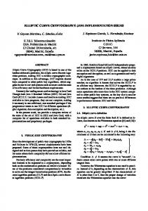
T[21] T[2 T[21] T[21]

T[2]

…

T[2]

T[2]

T[1]

T[0]

T[0]

T[1]

T[1] …

T[1]

T[2]

T[2 T[21] T[21]

…

T[0]

T[0]

T[0]

… T[21] T[2

C[42]

…

T[2] T[2

T

TL(a[0])

T

TU(a[0])

T

TL(a[1])

T

TU(a[1])

T

TL(a[2])

11

… T[1] T[1

T

T[0] T[0

…

C[2]

C[1]

C[0]

TU(a[20])

C

Fig. 1. Process of field multiplication using Alg. 2.

5

Proposed Techniques for Further Improvement

The performance of the field multiplication and reduction algorithms presented in Sect 4.2 can be improved by eliminating the redundant memory accesses. We can observe that both field multiplication and reduction algorithms are involved in a large number of memory access operations. Note that the memory access operations occupy large portion of the whole execution time. 5.1

Reducing Redundant Memory Accesses in Field Multiplication

Field multiplication over GF (2m ) is involved in many redundant memory accesses. This is the reason why typically the performance of field multiplication over GF (2m ) is inferior to that over GF (p). Fig. 1 describes the process of field multiplication using Alg. 2. In Fig. 1, odd rows are the intermediate result of the second for-loop and even rows are related to the first for-loop of Alg. 2. Later, all rows are XORed each other at corresponding positions to generate final result C (partial XOR multiplication). According to the Alg. 2, the result of the first for-loop shifts to left by window size (in our case, w = 4); it makes even rows to be shifted to the left direction depicted as Fig. 1. In each for-loop of Alg. 2, the L(a[j]) or U (a[j]) is evaluated to access the precomputed table about b(z). Afterwards, the corresponding element in the table is loaded and XORed with C from j to (j + N ) word (N = t). Observing the process of multiplication in Fig. 1 in detail, we can discover that the Alg. 2 is related to redundant memory accesses. The following example process shows the observation (we consider only the process of the second for-loop for the sake of simplicity). C0 ← C0 ⊕ T0 ; // C0 : 1 LOAD, T0 : 1 LOAD, STORE: 1 C1 ← C1 ⊕ T0 , C1 ← C1 ⊕ T1 ;

12

Seog Chung Seo et al.

Algorithm 5 Proposed left-to-right comb method using window width w = 4 1: 2: 3: 4: 5: 6: 7: 8: 9: 10: 11: 12: 13: 14: 15: 16: 17: 18: 19: 20: 21: 22: 23: 24: 25: 26: 27: 28:

INPUT: a(z) and b(z) in GF (2m ) OUTPUT: c(z) = a(z) · b(z) Compute Tu = u(z) · b(z) for all polynomials u(z) of degree at most w − 1. C ← 0. for j ← 0 to t − 2 increments j by 2 do u1 ← U (a[j]), u2 ← U (a[j + 1]). C[j] ← C[j] ⊕ Tu1 [0], C[j + N + 1] ← C[j + N + 1] ⊕ Tu2 [N ]. for i ← 1 to N increments i by 1 do C[i + j] ← C[i + j] ⊕ Tu1 [i] ⊕ Tu2 [i − 1]. end for end for u1 ← U (a[t − 1]). for i ← 0 to N increments i by 1 do C[i + t − 1] ← C[i + t − 1] ⊕ Tu1 [i]. end for C ← C · zw . for j ← 0 to t − 2 increments j by 2 do u1 ← L(a[j]), u2 ← L(a[j + 1]). C[j] ← C[j] ⊕ Tu1 [0], C[j + N + 1] ← C[j + N + 1] ⊕ Tu2 [N ]. for i ← 1 to N increments i by 1 do C[i + j] ← C[i + j] ⊕ Tu1 [i] ⊕ Tu2 [i − 1]. end for end for u1 ← L(a[t − 1]). for i ← 0 to N increments i by 1 do C[i + t − 1] ← C[i + t − 1] ⊕ Tu1 [i]. end for Return (c)

// C1 : 2 LOADs, T0 : 1 LOAD, T1 : 1 LOAD, STORE: 2 C2 ← C2 ⊕ T0 , C2 ← C2 ⊕ T1 , C2 ← C2 ⊕ T2 ; // C2 : 3 LOADs, T0 : 1 LOAD, T1 : 1 LOAD, T2 : 1 LOAD, STORE: 3 C3 ← C3 ⊕ T0 , C3 ← C3 ⊕ T1 , C3 ← C3 ⊕ T2 , C3 ← C3 ⊕ T3 ; // C3 : 4 LOADs, T0 : 1 LOAD, T1 : 1 LOAD, T2 : 1 LOAD, T3 : 1 LOAD, STORE: 4 ···

The calculations of C1 , C2 and C3 are related to two, three, and four STORE operations which are redundant. In addition to, Ci is loaded i + 1 times each step.5 Therefore, the running time of Alg. 2 can be decreased by reducing the number of STOREs and LOADs of Ci . Our strategy is to reduce the number of STOREs and LOADs which are related to XOR multiplications (C{j} ⊕ Tu ) by combining them. For example, we can combine “C{0} ⊕ TU (a[0]) ” and “C{1} ⊕ TU (a[1]) ” into “C{1} ← C{1} ⊕ TU (a[0]) {N, . . . , 1} ⊕ TU (a[1]) {N − 1, . . . , 0}, C[0] ← C[0] ⊕ 5

Ci is loaded i + 1 times until i ≤ 20, and is loaded 42 − i times during 20 < i ≤ 41.

TinyECCK

13

Table 2. Improved performance of the field operation in GF (2163 ) (L=LOAD, S=STORE, X=XOR. all timings are measured by secs). Field operation Existing Proposed Improvement (%) Time 0.00370277 0.00292224 21.08 Multiplication Operations 1,890L+966S+924X 1,430L+506S+924X 460L+460S saved Time 0.00034239 0.00025801 24.68 Reduction Operations 80L+80S+140X 50L+50S+140X 30L+30S saved

TU (a[0]) [0], C[N + 1] ← C[N + 1] ⊕ TU (a[1]) [N ]”.6 We formulate this strategy into Alg. 5. In fact, the more C{j} ⊕ Tu can be integrated at the expense of larger code size. In our case, we combine two XOR multiplications into one considering optimization between code size and performance; thus, the counter j of for-loops is incremented by 2. However, the final XOR multiplications, step 9 and 15 of Alg. 5, should be computed outside for-loops since the t is a odd number. Theoretical Analysis We can calculate the saved number of STOREs and LOADs in the proposed strategy. In the original algorithm, the counter j of for-loop is from 0 to (t − 1) and a C{j}⊕Tu consists of (t+1)(2L+S+X) operations (L=LOAD, S=STORE, X=XOR). Since the XOR multiplication is computed 2t times in the original algorithm, the total operations in the for-loops of the original algorithm are 2t[(t + 1)(2L + S + X) + (L + S)] = (4t2 + 6t)L + (2t2 + 4t)S + (2t2 + 2t)X (Additional (L+S) is used by u ← U (a[j]) or L(a[j])). On the other hand, in the proposed algorithm, the combined XOR multiplication requires [t(3L+S +2X)+ (4L + 2S + 2X)]. Since the combined XOR multiplication is processed (t − 1) times, the total operations of for-loops are (t − 1)[t(3L + S + 2X) + (6L + 4S + 2X)]+2[(t+1)(2L+S +X)+(L+S)] = (3t2 +5t+2)L+(t2 +3t+2)S +(2t2 +2t)X 7 . Therefore, (t2 + t − 2) of STOREs and LOADs are saved. Table 2 shows that we can significantly decrease the execution time with Alg. 5 replacing Alg. 2 by 21.1% and save (460S+460L) when t = 21. 5.2

Reducing Redundant Memory Accesses in Modular Reduction

The fast reduction modulo (Alg. 3) also involves many redundant memory accesses. Let us consider an example that the counter i decreases from 30 to 27 in the process of Alg. 3. Regarding the decrease of the counter (i.e., i = 6

7

In this process, only LOAD and STORE operations are reduced, not XOR operations. In case of sect163k1, t is odd number (t = 21). Therefore, the final XOR multiplication must be computed outside of for-loop (postprocessing steps: step 12–15 and 24-27 of Algorithm 5). The operations of the final XOR multiplications are 2[(t + 1)(2L + S + X) + (L + S)].

14

Seog Chung Seo et al.

Table 3. Improvement of overall performances with the proposed methods (TinyECCK uses sect163k1, all times are measured by secs.)

Sign Verify Sign Proposed Verify Sign Saving (%) Verify Original

Binary 5.4900 7.5789 4.4036 6.0825 19.78 19.74

2NAF 4.3061 5.9157 3.4718 4.7473 19.37 19.74

3NAF 3.8897 5.0642 3.1430 4.0750 19.19 19.53

4NAF 3.5750 4.5383 2.8949 3.6590 19.02 19.37

2TNAF 2.2003 4.2179 1.8287 3.4499 16.88 18.20

3TNAF 1.8770 3.3391 1.5745 2.7425 16.11 17.86

4TNAF 1.6111 2.7815 1.3613 2.3116 15.50 16.89

Table 4. The ratio of contribution between Alg. 5 and Alg. 6. The ratio is computed as (saved time from Alg. 5 or Alg. 6)/ (total saved time using Alg. 5 and Alg. 6). 2TNAF Sign Verify Alg. 2, Alg. 3 2.2003 4.2179 Alg. 2, Alg. 6 2.1043 4.0606 Alg. 5, Alg. 3 1.9230 3.6096 Alg. 5, Alg. 6 1.8287 3.4499 Alg. 5/(Alg. 5+Alg. 6) (%) 74.61 79.20 Alg. 6/(Alg. 5+Alg. 6) (%) 25.83 20.48 Used algorithms

3TNAF Sign Verify 1.8770 3.3391 1.7938 3.2073 1.6590 2.8805 1.5745 2.7425 72.06 76.87 27.49 22.10

4TNAF Sign Verify 1.6111 2.7815 1.5356 2.6725 1.4366 2.4224 1.3613 2.3116 69.85 76.42 30.20 23.20

30, 29, 28, 27), the execution steps are as follows: 1. T ← C[30]; 2. C[9] ← C[9] ⊕ (T ¿ 5); 3. C[10] ← C[10] ⊕ (T ¿ 4) ⊕ (T ¿ 3) ⊕ T ⊕ (T À 3); 4. C[11] ← C[11] ⊕ (T À 4) ⊕ (T À 5); 5. T ← C[29]; 6. C[8] ← C[8] ⊕ (T ¿ 5); 7. C[9] ← C[9] ⊕ (T ¿ 4) ⊕ (T ¿ 3) ⊕ T ⊕ (T À 3); 8. C[10] ← C[10] ⊕ (T À 4) ⊕ (T À 5); 9. T ← C[28]; 10. C[7] ← C[7] ⊕ (T ¿ 5); 11. C[8] ← C[8] ⊕ (T ¿ 4) ⊕ (T ¿ 3) ⊕ T ⊕ (T À 3); 12. C[9] ← C[9] ⊕ (T À 4) ⊕ (T À 5); 13. T ← C[27]; 14. C[6] ← C[6] ⊕ (T ¿ 5); 15. C[7] ← C[7] ⊕ (T ¿ 4) ⊕ (T ¿ 3) ⊕ T ⊕ (T À 3); 16. C[8] ← C[8] ⊕ (T À 4) ⊕ (T À 5);

Alg. 3 uses 16 STOREs and 16 LOADs to compute C[30], C[29], C[28], and C[27]. However, we can use the following strategy to reduce the redundant STOREs

TinyECCK

15

Algorithm 6 Proposed fast reduction modulo f (z) = z 163 + z 7 + z 6 + z 3 + 1 1: INPUT: A binary polynomial c(z) of degree at most 324 2: OUTPUT: c(z) mod f (z) 3: for i ← 41 to 21 decrements i by 4 do T1 ← C[i], T2 ← C[i − 1], T3 ← C[i − 2], T4 ← C[i − 3]. 4: 5: C[i − 24] ← C[i − 24] ⊕ (T4 ¿ 5). 6: C[i − 23] ← C[i − 23] ⊕ (T3 ¿ 5) ⊕ (T4 ¿ 4) ⊕ (T4 ¿ 3) ⊕ T4 ⊕ (T4 À 3). 7: C[i − 22] ← C[i − 22] ⊕ (T2 ¿ 5) ⊕ (T3 ¿ 4) ⊕ (T3 ¿ 3) ⊕ T3 ⊕ (T3 À 3) ⊕ (T4 À 4) ⊕ (T4 À 5). 8: C[i − 21] ← C[i − 21] ⊕ (T1 ¿ 5) ⊕ (T2 ¿ 4) ⊕ (T2 ¿ 3) ⊕ T2 ⊕ (T2 À 3) ⊕ (T3 À 4) ⊕ (T3 À 5). 9: C[i−20] ← C[i−20]⊕(T1 ¿ 4)⊕(T1 ¿ 3)⊕T1 ⊕(T1 À 3)⊕(T2 À 4)⊕(T2 À 5). 10: C[i − 19] ← C[i − 19] ⊕ (T1 À 4) ⊕ (T1 À 5). 11: end for 12: T1 ← C[21], T2 ← C[20]. 13: C[0] ← C[0] ⊕ (T1 ¿ 5) ⊕ (T2 ¿ 4) ⊕ (T2 ¿ 3) ⊕ T2 ⊕ (T2 À 3). 14: C[1] ← C[1] ⊕ (T1 ¿ 4) ⊕ (T1 ¿ 3) ⊕ T1 ⊕ (T1 À 3) ⊕ (T2 À 4) ⊕ (T2 À 5). 15: C[2] ← C[2] ⊕ (T1 À 4) ⊕ (T1 À 5). 16: C[20] ← C[20] & 0x07 17: Return C[20], . . . , C[2], C[1], C[0].

and LOADs. 1. T1 ← C[30], T2 ← C[29], T3 ← C[28], T4 ← C[27]; 2. C[6] ← C[6] ⊕ (T4 ¿ 5); 3. C[7] ← C[7] ⊕ (T4 ¿ 4) ⊕ (T4 ¿ 3) ⊕ T4 ⊕ (T4 À 3) ⊕ (T3 ¿ 5); 4. C[8] ← C[8]⊕(T4 À 4)⊕(T4 À 5)⊕(T3 ¿ 4)⊕(T3 ¿ 3)⊕T3 ⊕(T3 À 3)⊕(T2 ¿ 5); 5. C[9] ← C[9]⊕(T3 À 4)⊕(T3 À 5)⊕(T2 ¿ 4)⊕(T2 ¿ 3)⊕T2 ⊕(T2 À 3)⊕(T1 ¿ 5); 6. C[10] ← C[10] ⊕ (T2 À 4) ⊕ (T2 À 5) ⊕ (T1 ¿ 4) ⊕ (T1 ¿ 3) ⊕ T1 ⊕ (T1 À 3); 7. C[11] ← C[11] ⊕ (T1 À 4) ⊕ (T1 À 5);

In this case, the number of STOREs and LOADs is reduced from 16 to 10. Alg. 3 requires 20*4 = 80 STOREs and LOADs in the for-loop. However, the proposed method requires only 5*10 = 50 STOREs and LOADs, which results in the saving of 30 STOREs and 30 LOADs. Alg. 6 is the formulation of the proposed strategy. As Table 2 indicates, the execution time of modular reduction with Alg. 6 replacing Alg. 3 is decreased by 24.7%. Actually, we can extend the degree of combination. However, the deeper degree of combination is used, the more code size is required. Therefore, it is necessary to find the optimal degree. Throughout experiments, we found that the 4 is more appropriate than other degrees. We apply the two aforementioned strategies to implement TinyECCK. Table 3 depicts the improved performances when TinyECCK equipped with Alg. 5 and 6 instead of Alg. 2 and 3. When the proposed strategies are applied, the TinyECCK presents around 15% ∼ 19% saving in execution time. The improve-

16

Seog Chung Seo et al.

ment when TinyECCK uses wTNAF is lower than when it uses wNAF since ECDBL operation is replaced by some trivial squarings with wTNAF. Remarks The Algorithm 2, Loop-unrolled reduction modulo with 32-bit word size, presented in [17] is very similar to the proposed Alg. 6. However, the focus of [17] is to show that changing the reduction polynomial can improve the performance of reduction algorithm rather than to verify that unrolling techniques can reduce the redundant memory accesses. Therefore, the purposes and contributions of [17] are different from our proposals which aim at showing that the concept of unrolling techniques can be used in both field multiplication and reduction so as to reduce the number of redundant memory accesses. Furthermore, the improvement from Alg. 5 is bigger than that from Alg. 6. Thus,the main contribution of this paper is Alg. 5. Table 4 shows that the ratio of improvement from Alg. 5 occupies around 70% while that from Alg. 6 is only 20 ∼ 30%.

6

Experimental Results and Analysis

This section analyzes the performance of TinyECCK – in terms of running time, memory occupancy, and supporting services – and compares it with the performances of existing ECC software implementations. 6.1

Analysis of Field Operations

We compare TinyECCK with TinyECC [1] in the light of the running time of field operations to show that the field multiplication over GF (2m ) can be faster than that over GF (p) on sensor motes. TinyECC applies hybrid multiplication/squaring using additional registers to reduce unnecessary memory accesses and optimized modular reduction using pseudo-Mersenne prime. Thus it is fair to compare TinyECCK with TinyECC since TinyECCK also uses left-to-right comb method using window (Alg. 5) and fast reduction modulo (Alg. 6). Table 5 shows that the multiplication of TinyECCK is faster than that of TinyECC (the running time of multiplication and squaring includes the reduction time). In fact, the running time of field multiplication of TinyECCK is slower than that of TinyECC when using Alg. 2. However, with Alg. 5, TinyECCK’s field multiplication becomes faster than TinyECC’s one. Apart from the advantage of field inversion in TinyECCK, the field squaring in TinyECCK is much more efficient than that in TinyECC. 6.2

Consideration of Code Size

Even though TinyECCK implements the field arithmetics over both GF (2m ) and GF (p) to provide ECDSA services, it requires less code size than that TinyECC uses. Table 6 compares TinyECCK with TinyECC in view of the running time

TinyECCK

17

Table 5. Comparison of field operations between TinyECCK and TinyECC (for a fair comparison, the C version of TinyECC is compared with TinyECCK and all timings are measured by secs). Field operation Multiplication Squaring Inversion

TinyECC 0.00315647 0.00314779 0.14856858

TinyECCK Improvement (%) 0.00292224 7.42 0.00036982 88.25 0.07302550 50.84

Table 6. Performance Comparisons between TinyECCK and TinyECC (Time and code size are measured by secs and bytes, respectively).

Time Code Time Sign Code Time Verify Code SM

TinyECCK TinyECC (C) TinyECC (asm) 1.1411 6.1418 1.8825 5,592 8,528 10,092 1.3607 6.2694 2.0016 12,084 13,192 16,478 2.3237 7.9208 2.4318 13,748 15,872 19,308

[4]

[8]

[9]

[7]

[10]

[1]

TinyECCK (SM version)

Language

C

C with inline asm

C

C

asm

C with inline asm

Platform

Mica2 (Atmega128 8-bit)

TelosB (MSP430 16-bit)

Domain Parameter

sect163k1

secp160r1

sect163k1

sect113r1

sect163r1

secp160r1

sect163k1

Underlying Field

Binary

Prime

Binary

Binary

Binary

Prime

Binary

ROM size (byte)

34,342

17,823

11,592

RAM size (byte)

1,055

SM (secs)

C

Micaz Mica2 Atmega128 Atmega128 (Atmega128 (Atmega128 8-bit 8-bit 8-bit) 8-bit)

75,088

8,767

19,308

1,638

820

208

239

1,510

34.161

3.13

13.9

6.74

4.14

1.8825

Sign (secs)

-

3.35

-

6.88

-

2.0016 (init:1.83)

Verify (secs)

-

6.78

-

24.17

-

2.4318 (init: 3.49)

Supporting Protocols

SM, ECDH

SM, ECDSA

SM, ECDH

SM, ECDSA, ElGamal

SM

SM, ECDSA

TinyECCK (ECDSA version)

Micaz (Atmega128 8-bit)

13,748

5,592 618 (w = 4)

330 (w = 2)

1.1370 1.6852 (init: 0.0005) (init: 0.2515)

1,004 (w = 4) 1.1411 (init: 0.2514) 1.3613 (init: 0.2515)

-

2.3116 (init: 0.2449) SM, ECDSA

Fig. 2. Performance analysis of ECC implementations on sensor motes (asm and SM mean assembly code and scalar multiplication, respectively. All timings are measured by secs.)

18

Seog Chung Seo et al.

and the code size when they do same operations. TinyECC using inline assembly at the critical parts such as multiplication, squaring and reduction could achieve the improved performance at the expense of more code size, however it is still inferior to TinyECCK. Actually TinyECC implements hybrid multiplication/squaring algorithms which aim at reducing the number of memory accesses by using additional registers through inline assembly codes; thus the code size of TinyECC is highly increased. The code size of the scalar multiplication module in TinyECCK is only 5,592byte since the field multiplication and squaring can be simply implemented. However, ECDSA module of TinyECCK requires more code size in that signature generation and verification need additional field operations over GF (p). The code size for field arithmetics over GF (p) in TinyECCK is relatively smaller than that of TinyECC. This is because TinyECCK applies only a few optimization techniques for field arithmetics over GF (p) while TinyECC uses all known optimization algorithms. As shown in Table 6, TinyECCK is more faster and memory-efficient than TinyECC. The main reason that the code size of TinyECCK can be smaller than that of TinyECC is that TinyECCK presents better performance than implementations using inline assembly code even though it is built in only C code. TinyECCK does not need the use of inline assembly codes in that it presents good performance without applying them8 . Application of the proposed algorithms and wTNAF-based scalar multiplications contributes this performance achievement. Through this result, we can verify our assertion: the code size of the optimized ECDSA implementation over GF (2m ) can be smaller than that over GF (p). 6.3

Performance Comparisons

Fig. 2 analyzes the existing software implementations of ECC on sensor motes and compares the performance of TinyECCK with them in respect to various aspects such as running time, code size, supporting protocols, and so on. The performances of existing implementations of ECC over GF (2m ) [4, 9, 7, 10] are relatively low compared with [8, 1]. Even if ECC in [10] is implemented with assembly code, its performance is still inferior to [1] which is implemented with C and partially inline assembly. The implementations in [4, 9] could not exploit the advantages of Koblitz curve since they did not implement wTNAF recoding algorithm even if they used the sect163k1 as a domain parameter. The critical reason why TinyECCK can be the fastest among software implementations of ECC over GF (2m ) is that TinyECCK implements the wTNAF-based scalar multiplication and applies the proposed algorithms for field multiplication and reduction (Without applying signed recoding algorithms, the running time of TinyECCK is almost same as that of [10]). TinyECCK provides the improved performance in view of running time, used ROM and RAM size compared with 8

We expect that TinyECCK operates faster than now, if its performance-critical parts are implemented with inline assembly codes at the expense of larger code size.

TinyECCK

19

existing implementations. The modules for a scalar multiplication in TinyECCK require only 5,592-byte of ROM; 330-byte of RAM is occupied with 2TNAF, and 618-byte with 4TNAF. Moreover, its running time is also superior to the existing software implementations built in C or hybrid of C and inline assembly. Even if the ECDSA modules of TinyECCK require more code size (13,748-byte of ROM, 1,004-byte of RAM in case 4TNAF is applied) for the signature generation and verification, its code size is still smaller than that of TinyECC (19,308byte of ROM and 1,510-byte of RAM). Moreover, TinyECCK is better than TinyECC with regard to initialization time for establishing precomputed tables and initializing domain parameters. TinyECCK takes 0.2515 secs to compute a precomputed table when 4TNAF is applied, while TinyECC takes 1.83 secs to establish a precomputed table with 4-ary window method. With TinyECCK, two sensor nodes can compute a common pairwise key around 1.14 secs. Furthermore, a sensor node can generate a signature and verify it in 1.37 and 2.32 secs, respectively. In light of supporting protocols, TinyECCK provides modules for all elliptic curve operations over GF (2m ) from point addition, doubling and scalar multiplication to ECDSA services. Remarks After finishing our work, we have noticed the existence of NanoECC [19]. NanoECC provides the implementations of ECC and pairing-based cryptography (PBC) over GF (p) and GF (2m ) on both widely used MICA2 and Tmote Sky motes. NanoECC is based on MIRACL (Multiprecision Integer and Rational Arithmetic C/C++ Library) which provides all the necessary primitives and functions for symmetric-key and public-key cryptography. When implementing ECC over GF (2m ), NanoECC use the sect163k1 same as the curve TinyECCK uses. For the optimized field level arithmetics, NanoECC makes use of KaratsubaOfman multiplication and fast reduction algorithm using f (x) = x163 +x7 +x6 + x3 + 1. NanoECC implements the hybrid multiplication algorithm and a fast reduction algorithm using Solinas prime (p = 2160 − 2112 + 264 + 1) for efficient big integer arithmetic over GF (p). The elliptic curve points in NanoECC are represented as projective coordinate and the fixed-based comb method is applied for efficient scalar multiplications with w = 4 using 16 precomputed points. Table 7 compares TinyECCK with NanoECC. Even if NanoECC can compute scalar multiplication relatively fast compared with existing ECC implementations on the ATmega128L processor, it requires a heavy amount of ROM and RAM sizes. We think that the heavy memory requirement of NanoECC is due to using the MIRACL which is originally intended for efficient big number arithmetic on typical computer systems. On the other hand, TinyECCK has been developed with considering memory and computing-constrained environments of sensor motes. Therefore, TinyECCK using 4TNAF or 5TNAF provides better performance than NanoECC with regard to both computation times and memory requirements. However, the development of NanoECC is significant because it implements not only ECC but also pairing-based cryptography on widely used two

20

Seog Chung Seo et al.

Table 7. Performance Comparisons between TinyECCK and NanoECC on ATmega128L processor (Time and code size are measured by secs and bytes, respectively). TinyECCK NanoECC Using 4TNAF Using 5TNAF Binary field Prime field Scalar Multiplication (secs) 1.14 0.99 2.16 1.27 ROM (byte) 5,592 5,592 33,177 47,206 RAM (byte) 618 1,002 1,740 1,843

sensor motes (MICA2 and Tmote Sky). In case of PBC, NanoECC privides the fastest pairing computations.

7

Conclusion

In this paper, we have described that the inefficiency of field multiplication and reduction over GF (2m ) are caused by a heavy amount of redundant memory accesses. Therefore, we have proposed techniques to reduce unnecessary memory accesses. With the proposed techniques, running times of field multiplication and reduction over GF (2163 ) are saved as much as 21.1% and 24.7%, respectively. These savings decrease the running time of ECDSA operations around 15% ∼ 19%. The proposed multiplication algorithm is approximately 7.4% faster than hybrid field multiplication over GF (p). We have implemented TinyECCK with the proposed techniques on a MICAz sensor mote and compared it with the existing implementations built in C or hybrid of C and inline assembly. The comparisons show that TinyECCK provides more improved performance than the existing implementations in respect to running time, code size, and supporting services. From experimental results and comparisons, we obtain the two conclusions. Firstly, the software implementation of ECC over GF (2m ) is more suitable for sensor motes with small word size than that of ECC over GF (p). Note that this fact is contrast to existing opinions. Especially, the field multiplication over GF (2m ) can be faster than that over GF (p) with careful implementations. Secondly, the use of ECC, especially TinyECCK is applicable for securing sensor networks.

Acknowledgments “This research was supported by the MKE(Ministry of Knowledge Economy), Korea, under the ITRC(Information Technology Research Center) support program supervised by the IITA(Institute of Information Technology Advancement)” (IITA-2008-(C1090-0801-0025)).

TinyECCK

21

References 1. A. Liu, P. Kampanakis, and P. Ning, “TinyECC: Elliptic Curve Cryptography for Sensor Networks (Version 1.0),” available at “http://discovery.csc.ncsu.edu/software/TinyECC/,” November 2007. 2. C. Karlof, N. Sastry, and D. Wagner, “TinySec: Link Layer Security Architecture for Wireless Sensor Networks,” Proceedings of the 2nd International Conference on Embedded Networked Sensor Systems (SenSys’04) pp. 162–175, 2004. 3. Certicom Research, “SEC 2: Recommended Elliptic Curve Domain Parameters, Standards for Effcient Cryptography, Version 1.0,” September 2000. 4. D. J. Malan, M. Welsh, and M. D. Smith, “A Public-Key Infrastructure for Key Distribution in TinyOS Based on Elliptic Curve Cryptography,” In the first IEEE international conference on Sensor and Adhoc communications and Networks (SECON04), 2004. 5. D. Hankerson, J. L´ opez, and A. Menezes, “Software Implementation of Elliptic Curve Cryptography over Binary Fields,” Workshop on Cryptographic Hardware and Embedded Systems (CHES 2000), LNCS 1965, pp.1–24, 2000. 6. D. Hankerson, A. J. Menezes, and S. Vanstone, “Guide to Elliptic Curve Cryptography,” Springer-Verlag, 2004. 7. E. O. Blaß and M. Zitterbart, “Towards Acceptable Public-Key Encryption in Sensor Networks,” ACM 2nd International Workshop on Ubiquitous Computing, INSTICC Press, Miami, USA, May, pp. 88–93, 2005. 8. H. Wang, B. Sheng and Q. Li, “Elliptic curve cryptography-based access control in sensor networks,” International Journal of Security and Networks, Vol. 1, Nos. 3/4, 2006. 9. H. Yan and Z. Shi, “Studying software implementations of elliptic curve cryptography,” Third International Conference on Information Technology: New Generations (ITNG 2006), pp. 78–83, 2006. 10. H. Eberle, A. Wander, N. Gura, S. Chang-Shantz, and V. Gupta, “Architectural Extensions for Elliptic Curve Cryptography over GF (2m ) on 8-bit Microprocessors,” 16th International Conference on Application-Specific Systems, Architecture and Processors (ASAP 2005), Vol.00, pp. 343–349, 2005. 11. J. Solinas, “Efficient Arithmetic on Koblitz curves,” Design, Codes and Cryptography, 19:195–249, 2000. 12. J. L´ opez and R. Dahab, “Improved Algorithms for Elliptic Curve Arithmetic in GF (2n ),” Selected Areas in Cryptography (SAC’98), LNCS 1556, pp. 201–212, 1999. 13. J. L´ opez and R. Dahab, “High-Speed Software Multiplication in F2m ,” Progress in Cryptology – INDOCRYPT 2000, LNCS 1977, pp. 203–212, 2000. 14. MICAz Hardware Description Available at “http://www.xbow.com/Products”. 15. N. Gura, A. Patel, A. Wander, H. Eberle, and S. Chang-Shantz, “Comparing Elliptic Curve Cryptography and RSA on 8-Bit CPUs,” Workshop on Cryptographic Hardware and Embedded Systems (CHES 2004), LNCS 3156, pp. 119–132, 2004. 16. TinyOS forum. Available at “http://www.tinyos.net/”. 17. Michael Scott, “Optimal Irreducible Polynomials for GF (2m ) Arithmetic”, Cryptology ePrint Archive, Report 2007/192, 2007. 18. B. M¨ oller, “Improved Techniques for Fast Exponentiation,” Information Security (ISC 2002), LNCS 2587, pp. 298–312, 2003.

22

Seog Chung Seo et al.

19. Piotr Szczechowiak, Leonardo B. Oliveira, Michael Scott, Martin Collier, and Ricardo Dahab, “NanoECC: Testing the Limits of Elliptic Curve Cryptography in Sensor Networks,” European Wireless Sensor Networks (EWSN 2008) LNCS 4913, pp. 305–320, 2008,