Efficient Forward Dynamics Simulation and ... - Semantic Scholar

Preprint of the paper which appeared in Proc. AMAM 2005, Ilmenau, Germany, September 25-30, 2005

Efficient Forward Dynamics Simulation and Optimization of Locomotion: From Legged Robots to Biomechanical Systems Maximilian Stelzer and Oskar von Stryk Simulation and Systems Optimization Group Technische Universit¨at Darmstadt Darmstadt, Germany Email: @sim.tu-darmstadt.de www.sim-opt.de

Abstract— Locomotion of both walking robots and biomechanical systems show redundancies in the joint angle trajectory required to move the leg to a certain position and biomechanical systems additionally in muscle recruition. This paper shows the use of efficient dynamics modeling, dynamics algorithms and optimal control techniques to solve for optimal solutions to (goal oriented or measured reference) motions that as well solve the redundancy problems. Forward dynamics calculations are performed to solve both problems synchronously. A new approach proposed by the authors to the forward dynamics simulation and optimization problem outperforms commonly used methods by two orders of magnitude in numerical efficiency.

I. INTRODUCTION

II. WALKING ROBOTS AND BIOMECHANICAL SYSTEMS A. Characteristics of walking robots Walking robots are characterized by a high number of actuated or non-actuated joints, frequent changes in the kinematic structure due to switching contact situations (single or double limb support), and tree structure when contacts are cutted and treated separately. Actuation commonly is comparatively simple with walking robots: Each joint has at most one motor and each motor is directly connected to one joint. Motors itself are characterized by maximum (short-time or permanent) torque resp. current, angle constraints, gear ratio and axis inertias. Control variables therefore may be joint torques or motor currents. B. Biomechanical systems

Complex dynamic systems like walking robots need sophisticated approaches for generating stable motions. Although feedback control will be needed in most cases, basic (walking) trajectories (upon which the control layer may act) are essential. The approach we discuss in this paper is based on dynamics modeling and optimal control. Biomechanical systems’ actuation is more complicated than those of walking robots. Never the less, the techniques of walking robot trajectory optimization may be used to investigate biomechanical systems as well. The drawback of forward dynamics solution to the problem is its high numerical effort compared to inverse dynamics approaches. On the other hand it can handle much more general models. We show a new approach to forward dynamics computation that is faster by two orders of magnitude compared to methods used right now. The outline of the paper is as follows: Section II introduces the system components this paper deals with, Section III reviews an efficient dynamics algorithm for both walking robots and biomechanical systems. Optimization techniques used are presented in Section IV. Numerical and experimental results are presented in Section V. Section VI concludes the paper.

Biomechanical systems differ from walking robots in several points. One main difference lies in actuation: In biomechanics, joints are actuated by muscles, which primarily exert linear forces. Muscles may span over several joints and commonly one joint is connected to several muscles. Nevertheless tree structure may be conserved when muscles are assumed to have no mass or having its mass rigidly attached to the bones. Knowing the force insertion points (which depend on the joint angle, cf. muscle paths Section II-C.4), torques may be calculated and inserted directly into the problem. Controls for biomechanical system are the muscle activations (cf. Section II-C.3). Once the linear force for each muscle is determined, each joint’s torque is calculated taking into account the muscle path (Sections II-C.5, II-C.4). In contrast to the robots’ rigid links, biomechanical structures show high flexibility. Also the wobbling masses should be taken into account (but are not considered yet in this paper). Contact situation of human feet with the ground are much more complex than rigid robot’s feet’s contact with the ground. For the example of kicking investigated in Section V-B however, this is not necessary because there is no contact of the swing leg that has to be modeled at all.

1−

1.4

1.2

1.2

1

1

force−velocity factor

force−velocity factor

1.4

0.6

0.4

0 −1

−0.6

−0.4

−0.2

0

0.2

0.4

normalized muscle velocity

0.6

0.8

1

0.7

0.7

0.6 0.5 0.4

0.6 0.5 0.4

0.3

0.3

0.2

0.2 0.1

0.1 0 0.5

gamma fAD u

1

1.5

2

0 0

0.2

0.4

normalized muscle length

0.6

0.8

1

time

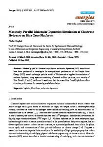
Fig. 2. Tension-length relation with c1 = 0.017 and c2 = 0.015.

Fig. 3. Activation dynamics with b1 = 7, b2 = 7, b3 = 1.

3) Activation dynamics: Muscles may not exert force instantaneously. Muscle excitation u leads to increased calcium ion concentration γ in the muscle which finally results in force exertion. This is modeled by: γ˙ = b2 (b3 u − γ) How the calcium ion concentration relates to the force exerted is given by the following equation: fAD (γ(u)) =

(b1 γ(u))3 1 + (b1 γ(u))3

The overall muscle activation dynamics is shown in Figure 3. 4) Muscle path: The muscle lengths and velocities needed for the relations above may be expressed by joint angles qi and joint angular velocity q˙i : = =

l(q1 , q2 , ...), v(q1 , q2 , ..., q˙1 , q˙2 , ...)

0.8

0.6

0.2

−0.8

0.8

lM vM

0.4

0.2

1 0.9

0.8

M vmax c4

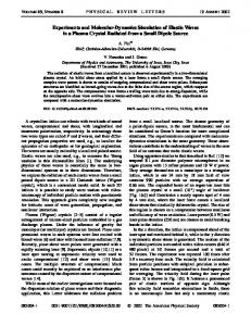
Figure 1 shows two examples of the force-velocity relation for a fast and a slow muscle.

0.8

1 0.9

activation dynamics

Each muscle shows some characteristic behavior due to its structure. We review the resulting relations ([22]) and short explanations for them; the structure itself shall not be reviewed here. The relations give factors to be multiplied with the maximum isometric force. 1) Force-velocity relation: The active force a muscle may exert depends on its velocity. It is equal to the muscle maximum isometric force at zero velocity and equal to zero at the maximum contraction velocity. The active force is higher than the maximum isometric force if the muscle has excentric velocity. The overall relation not only depends on the maximum velocity but also on parameters c3 , c4 that indicate how fast the force converges to zero with contractive velocity resp. how fast the force converges to the maximum force with excentric velocity. For fast muscles c3 ∈ [0.25, 1], while for slow muscles, c3 ∈ [0.1, 0.25]. The overall force-velocity relation is given by:  M 1− vM  vmax   , vM ≤ 0 M  1+ v  M  v c max 3 ¡ ¢ fF V v M =  M  1−1.33 Mv  vmax c4   , v M > 0.  M v

tension−length factor

C. Muscle modeling

0 −1

−0.8

−0.6

−0.4

−0.2

0

0.2

0.4

0.6

0.8

1

normalized muscle velocity

Fig. 1. Force-velocity relation for a slow (c3 = 0.1, c4 = 0.02; left) and a fast (c3 = 1.0, c4 = 0.1; right) muscle.

2) Tension-length relation: Muscle forces result from biochemical structures that grip into each other and thereby cause the movement respective force. It is obvious, that the more overlapping structures exist, the higher are the forces that may be established. If the muscle is expanded, less overlapping area and thus less potential force exists. If the muscle on the other hand is shortened, the structures obstruct each other and also less force may be exerted. This is modeled with the following equations, where c1 and c2 are parameters for the effect of decrease of forces when expanding resp. shortening the muscle:  M − c1 (1− l M )3  1.1l0 1  , lM ≤ 1.1l0M e ¡ M¢  fT L l =  3 lM   − c12 ( 1.1l M −1) 0 e , lM > 1.1l0M Figure 2 gives an example of the relation.

To calculate the torques that result from the linear muscle forces, the muscle path, i.e. the force insertion points and force exertion direction (or the resulting lever arm directly), have to be modeled. Anyway the resulting lever arm depends on the joint angles only (the first index i indicates the number of the muscle or muscle group, the second index j the number of the joint, the muscle has effects on; not all combinations of i, j are needed): di,j = di,j (q1 , q2 , ...). 5) Total muscle force: With the factors given in the previous section, the total muscle force may be stated as: iso F (γ, lM , v M ) = Fmax fAD (γ)fT L (lM )fF V (v M ).

6) Resulting active torques: The torque in joint j that results from the muscle forces is (with appropriate index sets Ij that indicate which muscles do effect to joint j): X τj,a = di,j Fi (γi , liM , viM ). i∈Ij

7) Passive torques: In addition to the active torques, passive torques have to be considered. Passive torques depend on lM , v M , γ (bold letters indicate the vector of all occurring lengths, velocities, calcium ion concentrations), and the joint angles. They model passive effects of tendons, ligament and

the connective tissue (especially at the boundaries of the feasible joint angle intervals) [11], [31]: τj,p = τj,p (lM , v M , γ, q). The total torque applied to joint j is τj = τj,a + τj,p Note that for robotic systems u is the torque and is equal to the control in the optimal control problem if no detailed motor model is used. For biomechanical systems u is the control (i.e. the muscle activations) and τ = (τ1 , τ2 , ...) are the torque for the dynamics calculations. III. DYNAMICS ALGORITHMS A. Dynamics algorithms for tree structured systems The basic equations of motion are those for a rigid, multibody system (MBS) experiencing contact forces ³ ´ q¨ = M(q)−1 Bu − C(q, q) ˙ − G(q) + Jc (q)T f c 0 = g c (q) where N equals the number of links in the system, m equals the number of actively controlled joints, M ∈ RN ×N is the square, positive-definite mass-inertia matrix, C ∈ RN contains the Coriolis and centrifugal forces, G ∈ RN the gravitational forces, and u(t) ∈ Rm are the control input functions which are mapped with the constant matrix B ∈ RN ×m to the actively controlled joints. The ground contact constraints g c ∈ Rnc represent holonomic constraints on the system from which ∂g the constraint Jacobian may be obtained Jc = ∂ qc ∈ Rnc ×N , while f c ∈ Rnc is the ground constraint force. q, q, ˙ and q¨ ∈ R are the generalized position, velocity and acceleration vectors respectively. These equations may be established with several algorithms. We use articulated body algorithm (ABA) due to its numerous advantages over other methods. ABA is a recursive numerical algorithm of order N (with N the number of links in the MBS). Because the systems we look at are generally of very high dimension, recursive algorithms can show their advances in computational effort compared to non-recursive methods [27]. ABA is tailored to tree structured, fully three dimensional systems and shows a high flexibility in exchange of parts of the model (kinematic and kinetic data, actuation, contact situations). ABA may be formulated analytically in operator formulation, which due to the special stacked structure of the operators involved numerically may be realized by recursive calculations in three sweeps from base to tip and vice versa [7], [21]. Additional sweeps may be added to handle contact forces and sensitivity information. The main idea of the algorithm lies in the fact that the mass matrix may be inverted explicitly using a factorization of the mass matrix: M = (I − KΘH)T D(I + KΘH), M−1

= (I − KΨH)D−1 (I + KΨH)T ,

where the occurring operators have physical interpretations [16]. A review of all the occurring operators, the recursive

algorithm and an approach for an object oriented implementation of the algorithm tailored to its structure may be found in [12]. B. Sensitivities Information about sensitivities are essential not only for numerical optimization but also for non-linear analysis, parameter identification and calibration. Exact sensitivities are superior to approximations (e.g. by finite differences) but often not available at reasonable cost. Jain [15] showed that in the operator formulation sensitivity information may be gained at low cost from ABA. The resulting iterative algorithms provide sensitivity information. Manipulator Jacobian may be calculated as well as sensitivities of inverse dynamics ∂u and forward dynamics ∂ q¨ w.r.t. position, velocity and control variables for tree-structured rigid MBS: ∂u = ∇q u∂q + ∇q˙ u∂ q˙ + ∇q¨u∂ q¨, ∂ q¨ = ∇u q¨∂u + ∇q q¨∂q + ∇q˙ q¨∂ q. ˙ The occurring partial derivatives may be stated in stacked operator notation. The resulting recursive algorithm is an extension of the forward dynamics recursive algorithm with modified inboard sweep and two additional sweeps. IV. OPTIMIZATION TECHNIQUES A. Forward vs. inverse dynamics solution Simulation of a time dependent behavior of a human movement modeled with the techniques stated in Section III not only means numerical integration of a high dimensional ODE system but also the solution of a static or dynamic optimization problem for the redundant muscle groups involved. If you consider a sequence of static postures of a movement this results in a sequence of static optimization problems. Their solution however only for slow movements give approximations of acceptable quality to the solution of the dynamic optimization problem over the whole time horizon of the movement (i.e. to the optimal control problem) [2], [9]. a) Inverse dynamics simulation and optimization: Inverse dynamics simulation for a given, e.g. measured movement calculates the muscle activations of the muscles involved under the assumption of certain criteria for solving the redundancy problem. By this approach practically only given movements may be analyzed; new movements may not be calculated and goal oriented movements (e.g. reaching certain joint angles) may not at all or may only very limitedly be optimized, e.g. [5]. Approaches to extend inverse dynamics simulation to the optimization of human movements rely on very specialized assumptions (like min/max criteria) to the objective function for solving the redundancy problem of the muscles and use a low dimensional parameterization of the free parameter space to efficiently solve the resulting optimization problem numerically [19], [20]. For slow movements dynamic properties of wobbling masses have no effect to the quality of the solution and only

for slow movements special min/max-criteria for solving the redundancy problem of the human musculoskeletal system on muscle-tendon-level may be justified. The overall forces and torques at one joint then are distributed to the muscles according to different parameters of the muscles. But if faster movements shall be investigated other optimality criteria have to be used. From the biomechanics point of view not only faster movements but also other optimality criteria are of interest. By now there are no methods to solve these problems with inverse dynamics simulation satisfactorily. First approaches to the efficient treatment of loops of parallel muscles, may be found in [17]. Inverse dynamics however here also is not solved for any general optimality criterion. In a two-level algorithm first the joint torques and then the muscle forces are calculated. b) Forward dynamics simulation and optimization: With forward dynamics simulation, in contrast, analysis of given movements as well as the calculation and optimization of free movements is possible. Starting with the muscle activations (that are to be determined) forward dynamics simulation calculates the resulting movement. By forward dynamics simulation it is possible to analyze movements of parts of the human body or the whole body if the resulting high dimensional nonlinear optimal control problems can be solved efficiently. One advantage of analyzing human movements with forward dynamics simulation is that differences of measured and calculated movements may be integrated into the optimality criterion which allows compensation of measurement errors (e.g. [25]), while with inverse dynamics simulation small measurement errors for a measured trajectory may result in large errors of the computed muscle forces. B. Common approaches to forward dynamics optimization Up to now numerical optimization using forwards dynamics simulation is commonly treated by methods that are not optimally tailored to the problem’s structure. Most methods transform the optimal control problem into a finitedimensional, constrained, nonlinear optimization problem (NLP) by parameterization of the controls [1,3,17,18,26] (a so-called direct shooting approach [30]). The resulting NLP is usually solved using sequential quadratic programming methods. For numerical calculation of the gradients of the objective function and constraints w.r.t. the optimized parameters the sensitivity matrix of the solution of the system of differential equations w.r.t. the optimized parameters has to be computed. For human movements this is usually done by external numerical differentiation with differences approximation which is a numerically quite expensive approach [17,18,26] because the differential equations of the system have to be integrated numerically at least as often as grid points in the discretization of the controls exist. This leads to overall very high computing times for movements with a higher number of muscle groups. The accurancy of the computed gradient approximation is

limited by the integration method and the forward difference truncation error. For example the computing times for human jumping with a leg model with 9 muscle groups and three joints [25], [6] have been reported to be in the region of days on a workstation in 1996 [23]. For a three-dimensional model of the whole body with 54 muscle groups computing times on workstations in the region of months have also been reported [1]. In [3] computing times are compared when using MIMD parallel computers and vector parallel computers. The method from [18] is used for a 14 dof model with 46 muscle-tendon groups. Computing times were up to three month on a normal computer (SGI Iris 4D25), 77 h on a vector parallel computer and 88 h on a MIMD parallel computer. The problem investigated in Section V-B with 2 joints and 5 muscle groups required computing time in the region of several hours on 1996’s workstations [24]. C. Efficient forward dynamics optimization using direct collocation A direct collocation method [29], [30], [28] is used to solve the resulting optimal control problems. States and controls are approximated by piece cubic resp. linear polynomials on a time discretization grid which can be refined successively. By a collocation approach the differential equations and nonlinear implicit and boundary conditions are transcribed to a nonlinear problem with the piecewise coefficients as variables. The resulting NLP is solved using efficient sequential quadratic programming method SNOPT ([8]), which exploits sparsity in NLP gradients and Jacobians that is a result of the special structure of the piecewise polynomial discretization. Using the direct collocation approach the differential equations are solved synchronously to the optimization, i.e. there is no need to integrate the differential equations several times to get gradient information. This results in a much more efficient forward dynamics calculation. D. Use of sensitivity information The sequential quadratic programming method SNOPT does not need user defined derivative information, but may also approximate derivatives by difference approximation. However, exact derivatives are useful for robustness and efficiency. First experiments comparing results with SNOPT’s derivatives and exact sensitivities gained from the dynamics algorithm [12] showed slight improvements in computation time and convergence ([13], [14]). V. NUMERICAL AND EXPERIMENTAL RESULTS A. Robotics: Walking robots Walking trajectories for both a four legged (see Figure 4) and a humanoid robot (Figure 6, the robot was constructed in joint work with a group from TU Berlin, now TU Munich) have been optimized ([26], [4]). Experimental results matched the calculated trajectories very well. Sequences of the obtained gaits are shown in Figures 5 and 7.

z x

y

z

z

x

x

y

q

1 right side view

q2

y

front view x

q3

Fig. 4. The four-legged Sony robot (left) and the kinematical structure of one leg (right). Fig. 7.

Snapshots of a step sequence.

controls as follows:    q1  q2        q˙1       q ˙ = x =   2   γ1        ...  γ5    u1 u =  ...  =  u5

Fig. 5.

Four scenes from an animation of a computed trot gait.

B. Biomechanics: Kicking motion A time optimal kicking movement has been investigated. Kinematic and kinetic data of the musculoskeletal system as well as muscle model parameters and measured reference data have been taken from Sp¨agele [22,25], whose data is based on those of Hatze [10]. The model (cf. Figure 8) consists of two joints, two rigid links and five muscle groups. The problem is formulated in a first order form x˙ = f (x, u, t) as an optimal control problem with 9 states and 5

personal computer

80 75

M8

M7

70 65

z

60

height 80 cm

55 50

batteries




 

45 40

M6



 

 

M5 35











y z

M9 M4

revolute 30 joint 25 20

M3

x

15 10

motion control board

M2 5

M1

0

−30 −25 −20 −15 −10

Fig. 6.

−5

0

5

10

15

20

25

30

35

40

45

50

Humanoid Kinematic Structure.

0

5

10

15

20

 hip angle  knee angle   hip velocity  , knee velocity  ca2+ concentration muscle 1    ... ca2+ concentration muscle 5  activation of muscle 1  ... activation of muscle 5

The kicking movement was optimized with respect to elapsed time, i.e. the merit function is Φ(x(tf ), tf ) = tf . Compared to the measured motion trajectories (and the results of [22], [25], which match the measured data very well), our results show a shorter time and higher maximum angles (Figure 10). The reason is, that in [22] the maximum muscle forces were modified to match the optimized time of the measurement. Obviously our optimal movement is another local minimum. Nevertheless, the controls (Figure 11) show the same characteristics. Computing time and size of the resulting NLP are shown in table 9. The direct shooting approach used in [22], [25] for 11 grid points required in the region of hours to compute the solution ([24]). Comparing the computing time with our approach (Figure 9) and considering how computational speed has progressed since 1996, we still obtain a speed up of two orders of magnitude. VI. CONCLUSIONS AND OUTLOOK We reviewed efficient numerical multibody systems dynamics algorithms and optimization techniques that allow solving the forward dynamics optimization in biomechanics in a general form two orders of magnitude faster than present methods. Future work includes refinements of the model: • wobbling masses and • a contact situation of the foot, which shall be modeled by a detailed foot model. Further motions of larger parts of the human body or of the complete human body shall be investigated. Measurements

81

829

129

531

1

1

0.8

0.8 muscle 2

60

0.6 0.4 0.2

6.3 s

Fig. 9. Size of the resulting NLP and computation time on a 1700 MHZ+ Athlon XP for two different numbers of grid points in the discretization of the proposed approach.

0

0

0.1

0.2

1.2

0.8

0.3

0.4

0

0.5

0

0.1

0.2

1

1 0.8

0.6 0.4

0

0.3

0.4

0.5

0.3

0.4

0.5

time

0.8

measured optimized

1

0.4

time

0.6 0.4 0.2

0.2 0.9

0.6

0.2

muscle 4

1.2 s

muscle 3

Fig. 8. Kinematic structure of the leg with 5 muscle groups.

10

muscle 1

grid points nonlinear constraints nonlinear variables computing time

0

0.1

0.2

0.3

0.4

0.5

0

0

0.1

0.2 time

time

0.7 0.8

1 knee angle

hip angle

0.6 0.5 0.4

0.6

EMG (controls) 0.8

0.4

calciom ions concentration muscle 5

0.3 0.2 0.2 measured optimized

0.1 0

0

0.05

0.1

0.15

0.2

0.25 time

0.3

0.35

0.4

0.45

0

0.5

−0.2

0

0.05

0.1

0.15

0.2

0.25 time

0.3

0.35

0.4

0.45

0.5

0.6 0.4 0.2 0

Fig. 10.

Hip (left) and knee (right) angle trajectories for kicking motion.

of joint angle trajectories, ground reaction forces and the anthropometric data of the proband supplied from cooperating groups will be used to investigate muscle activations for given motion. The methods presented in this paper are already capable in principle of handling this class of problems. ACKNOWLEDGMENT This work has been supported by the German Research Foundation (DFG) under grant STR 533/3-1 and the Research Center Computational Engineering of the TU Darmstadt. R EFERENCES [1] F. C. Anderson and M. G. Pandy. A dynamic optimization solution for vertical jumping in three dimensions. Comp. Meth. Biomech. Biomed. Eng., 2:201–231, 1999. [2] F. C. Anderson and M. G. Pandy. Static and dynamic optimization solutions for gait are practically equivalent. Journal of Biomechanics, 34:153–161, 2001. [3] F. C. Anderson, J. Ziegler, M. G. Pandy, and R. T. Whalen. Application of high-performance computing to numerical simulation of human movement. Journal of Biomechanic Engineering, 117:155–157, 1995. [4] M. Buss, M. Hardt, J. Kiener, J. Sobotka, M. Stelzer, O. von Stryk, and D. Wollherr. Towards an autonomous, humanoid, and dynamically walking robot: Modeling, optimal trajectory planning, hardware architecture, and experiments. In Proc. IEEE/RAS Humanoids 2003, to appear. Springer-Verlag. [5] M. Damsgaard, S.T. Christensen, and J. Rasmussen. An efficient numerical algorithm for solving the muscle recruitment problem in inverse dynamics simulations. In International Society of Biomechanics, XVIIIth Congress, July 8-13, 2001, Zurich, Switzerland, 2001. [6] P. Eberhard, T. Sp¨agele, and A. Gollhofer. Investigations for the dynamical analysis of human motions. Multibody System Dynamics, 3:1–20, 1999. [7] R. Featherstone. The calculation of robot dynamics using articulatedbody inertias. The Int. J. Robotics Res., 2(1):13–30, 1983. [8] P.E. Gill, W. Murray, and M.A. Saunders. SNOPT: An SQP algorithm for large-scale constrained optimization. SIAM Journal on Optimization, 12:979–1006, 2002.

0

0.1

0.2

0.3

0.4

0.5

time

Fig. 11. Results from optimization: Controls (corresponding to EMG) and calcium ions concentrations.

[9] R. Happee. Inverse dynamic optimization including muscular dynamics, a new simulation method applied to goal directed movements. Journal of Biomechanics, 27:953–960, 1994. [10] H. Hatze. The complete optimization of a human motion. Mathematical Biosciences, 28:99–135, 1976. [11] A. L. Hof and J.W. van den Berg. EMG to force processing II: estimation of parameters of the hill muscle model for the human triceps surae by means of a calferometer. Journal of Biomechanics, 14:759–770, 1981. [12] R. H¨opler. A unifying object-oriented methodology to consolidate multibody dynamics computations in robot control. PhD thesis, Technische Universit¨at Darmstadt, 2004. [13] R. H¨opler, M. Stelzer, and O. von Stryk. Integrated, object-oriented dynamics modeling for design, trajectory optimization, and control of legged robots. In Proc. Euromech 452 – Advances in Simulation Techniques for Applied Dynamics, Halle, Germany, 2004. [14] R. H¨opler, M. Stelzer, and O. von Stryk. Object-oriented dynamics modeling for legged robot trajectory optimization and control. In Proc. IEEE Conf. on Mechatronics and Robotics (MechRob), pages 972–977, Aachen, September 13-15 2004. [15] A. Jain and G. Rodriguez. Linearization of manipulator dynamics using spacial operators. IEEE Trans. Syst., Man, Cybern., 23(1):239–248, 1993. [16] A. Jain and G. Rodriguez. Diagonalized Lagrangian robot dynamics. IEEE Trans. Robotics and Automat., 11:571–584, 1995. [17] Y. Nakamura, K. Yamane, I. Suzuki, and Y. Fujita. Dynamic computation of musculo-skeletal human model based on efficient algorithm for closed kinematic chains. Proc. of the 2nd International Symposium on Adaptive Motion of Animals and Machines, Kyoto, March 4-8, 2003, 2003. [18] M. G. Pandy, F. C. Anderson, and D. G. Hull. A parameter optimization approach for the optimal control of large-scale musculoskeletal systems. Journal of Biomechanical Engineering, 114:450–460, 1992. [19] J. Rasmussen, M. Damsgaard, and S. T. Christensen. Optimization of human motion: to invert inverse dynamics. Intern. Society of Biomechanics, XVIIIth Congress, July 8-13, 2001, Zurich, Switzerland, 2001. [20] J. Rasmussen, M. Damsgaard, and M. Voigt. Muscle recruitment by

[21] [22] [23] [24] [25] [26]

[27] [28]

[29]

[30] [31]

the min/max criterion? a comparative numerical study. Journal of Biomechanics, 34(3):409–415, 2001. G. Rodriguez, K. Kreutz-Delgado, and A. Jain. A spatial operator algebra for manipulator modeling and control. International Journal of Robotics Research, 10(4):371–381, 1991. T. Sp¨agele. Modellierung, Simulation und Optimierung menschlicher Bewegungen. PhD thesis, Universit¨at Stuttgart, 1998. T. Sp¨agele. personal communication. 2002. T. Sp¨agele. personal communication. 2005. T. Sp¨agele, A. Kistner, and A. Gollhofer. Modelling, simulation and optimisation of a human vertical jump. Journal of Biomechanics, 32(5):521–530, 1999. M. Stelzer, M. Hardt, and O. von Stryk. Efficient dynamic modeling, numerical optimal control and experimental results for various gaits of a quadruped robot. In CLAWAR 2003: Intern. Conf. on Climbing and Walking Robots, Catania, Italy, Sept. 17-19, pages 601–608, Aachen, 2003. W. Stelzle, A. Kecskem´ethy, and M. Hiller. A comparative study of recursive methods. Archive of applied mechanics, 66(1–2):9–19, 1995. O. von Stryk. Numerical solution of optimal control problems by direct collocation. In Optimal Control - Calculus of Variations, Optimal Control Theory and Numerical Methods, volume 111, pages 129–143. Birkh¨auser, 1993. O. von Stryk. User’s guide for DIRCOL version 2.1: A direct collocation method for the numerical solution of optimal control problems. Technical report, Fachgebiet Simulation und Systemoptimierung, Technische Universit¨at Darmstadt, 2001. http://www.sim.informatik.tudarmstadt.de/sw/dircol. O. von Stryk and R. Bulirsch. Direct and indirect methods for trajectory optimization. Annals of Operations Research, 37:357–373, 1992. Y. S. Yoon and J. M. Mansour. The passive elastic moment at the hip. Journal of Biomechanics, 15:905–910, 1982.