Ef.ficient Groundwater Remediation System Design Subject to Uncertainty Using Robust Optimization Karen L. Ricciardi 1 ; George F. Pinder; and George P. Karatzas 3
Abstract: Many groundwater remediation designs for contaminant plume containment are developed using mathematically based groundwater now models. These mathematical models are most eiTective as predictive tools when the parameters that govern groundwater flow are known with a high degree of certainty. The hydraulic conductivity of an aquifer, however, is uncertain, and so remediation designs developed lIsing models employing one realization of the hydraulic conductivity field have an associated risk of failure of plume containment. To account for model uncertainty attributable to hydraulic conductivity in detennining an optimal groundwater remediation deSign for plume containment, a method of optimization called robust optimization is utilized, This method of optimization is a multi scenario approach whereby mUltiple hydraulic conductivity fields are examined simultaneously. By examining these fields simultaneously, the variability of the uncertainty is included in the model. To increase the efficiency of the robust optimization approach, a sampling technique i.'> developed that allows the modeler to determine the minimum number of field realizations necessary to achievc a reliable remediation design. 001: 10.1 06J/(ASCE)0733-9496(2007) 133:3(253) CE Database subject headings: Ground-water management; Operation costs; Optimization; Optimization models; Algorithms; Hydrology; Hydrologic models; Remedial action; Uncertainty principles.
Introduction Many active pump and treat groundwater-remediation designs, whether generated through the process of trial and error or by automated methods, are based upon groundwater models that use spccified aquifer parameters (Gorelick 1983; Ahlfeld et a1. 1988; Karat/as and Pinder 1993; Guan and Aral 1999). Etlorts are often made to quantify the reliability of these models through sensitiv ity and uncertainty analysis (Konikow and Mercer 1988). Through uncertainty analysis, research has shown that it is pos sible to reduce the uncertainty in a groundwater flow model through strategic data collection (Wang and McTernan 2002). The hydraul ic conductivity of a single hydrostratigraphic unit is spa lially variable (Gclhar 1993) and because of this fact, the reduc lion of uncertainty in groundwater models is limited. The hydraulic conductivity of an aquifer is the primary param eter that affects the results of a groundwater flow model. Even when adequate characterization of the spatial variability of hy draulic conduc:tivily has been obtained through data collection, modelers are still limited in their ability to represent a spatially 'Depl. of Mathematics, Univ. of :-"1assachusetts in Boston, 100 Morrissey Blvd., Boston, MA 02125. E-mail:
[email protected]
'Dept. (If Civil and Environmental Engineering, Univ. of Vermont, Burlmglol1, VT 0540 I. E-mail:
[email protected] 'Dept. of Environmental Engineering, Technical Univ. of Crete, GR- 100 Chama, Greece. E-mail:
[email protected] Notc. Di,t;lbslon open until October 1, 2007. Separate discussions must be submitted for individual papers. To extend the closing date by one month, a written request must be filed with the ASCE Managing Editor. The manuscript for this paper was submitted for review and pos sible publication on March 25, 2005; approved on April 19, 2006. This paper parl of the Journal of Water Resources Plllnning and Manage ment, Vo'. 133. "lo. 3, May 1,2007. ©ASCE. ISSN 0733-9496/2007/3 253-2()3/SZS.00
variable hydrostratigraphic unit due to the uncertainty associated with those areas where data have not been collected. Reliability studies examine the relationship between an L111Cer tain input parameter, and the effcct that this uncertainty has on the model, by comparing the probability density functions (PDFs) of the input parameter and the model results, A number of reliability studies related to hydrologic models have been conducted (Koni kow and Mercer 1988; Wagner 1999; Yenigul et al. 2006), Sen sitivity studies conducted on hydrologic models address how small variations in the input parameters affect the model results (Ahlfeld et al. 1988; Hamed et al. 1996). The results of sensitivity studies can be used to evaluate the significanee of various input parameters. Through sensitivity and reliability studies, it has been shown that remediation design models are very sensitive to changes in hydraulic conductivity and that there is a strong rela tionship between the uncertainty of hydraulic conductivity and the uncertainty in model results (Gorelick 1989; Gelhar 1993; Hamed et al. 1996). It is possible to include the uncertainty of hydraulic conduc tivity into groundwater flow analysis by llsing a multi scenario method such as a Monte Carlo approach (Hamed et al. 1996; Yenigul et a1. 2006). In the Monte Carlo approach, multiple real izations of hydraulic conductivity fields are randomly generated within the bounds of the unccrtainty parameters provided. The groundwater model is simulated for each realization, and the re sults from these models are examined collectively. The Monte Carlo approach is most often used to model groundwater flow and contaminant transport and in reliability studies, Stochastic methods have been applied in a variety of manners to incorporate the uncertainty in the aquifer's properties into groundwater management problems. A type of stochastic pro gramming called chance-constrained modeling was used in carly efforts to include uncertainty directly into optimal rcmediation designs (Tung 1986). These models utilize a technique whereby
JOURNAL OF WATER RESOURCES PLANNING AND MANAGEMENT © ASCE / MAY/JUNE 2007/253
the domain of the uncertain parameter value, in other words all possible values of this parameter, is determined through analysis of the associated PDF. A particular percentile of the distribution, whichever value produces an appropriate conservative result, is then used in a deterministic model. This minimum or maximum value equates with a particular percentile of the data. Wagner and Gorelick (1987), under the hypothesis of normality, split water quality constraints into two parts: a deterministic, expected value component, and a stochastic one related to a specified reliability level. By doing such, they were able to account for the variability in the uncertain parameters in a chance-constrained model. Opti mization models developed through stochastic programming often result in conservative systems. Genetic algorithms (GA) have also been used as a solution technique in the development of a robust approach to optimal groundwater remediation design that takes into account the uncer tainty of hydrauli.: .:onductivity values (Hilton and Culver 2005). Within each generation of the robust GA. all designs are evalu ated using the same realization of the heterogeneous hydraulic conductivity field, but the realizations vary between GA itera tions. Ongoing performance of the designs is measured and is used in the GA evolution process resulting in a conservative re mediation design that takes into account the uncertainty in hy draulic conductivity. Wagner et al. have simultaneously considered the operation of a pumping design for groundwater containment as well as the uncertainty in the aquifer properties through the application of a stochastic program with simple recourse (Wagner et al. 1992). This approach is a multi scenario stochastic programming ap proach, which may be considered a precursor to the robust opti mization approach utilized in this work. This model minimized the expected total costs of remediation over a number of realiza tions of outcomes of the random parameter, namely the hydraulic conductivity of the aquifer. This approach considers the uncer tainty in an explicit manner, resulting in a single remediation design that includes the data from the mUltiple realizations repre sentative of the uncertainty. Robust optimization (RO) is a multi scenario approach that can be used to develop a least-cost pump-and-treat-remediation de sign or redesign for containment of a contaminated aquifer sub ject to parameter uncertainty (Mulvey et al. 1995; Karatzas and Pinder 1997; Watkins and McKinney 1995). The RO approach analyzes, simultaneously, simulations that use a number of differ ent aquifer parameter values, thereby including the variance of the uncertain parameter in the model. Mulvey presented his vision of the RO algorithm, not by defining a set of rules, but rather by presenting the ideas for including uncertainty in the optimization problem. Mulvey states that there are multiple ways in which the RO approach can be implemented. This paper presents one pos sible implementation of the RO algorithm and how this approach can be cfficiently applied to the contaminant containment problcm. Robust optimization was first explored as a method for devel oping a risk-based groundwater remediation system by Watkins and McKinney in 1995 (Watkins and McKinney 1995, 1997). In this new application of Mulvey's approach, RO was used to quan tify the risk associated with pump and treat groundwater remedia lion designs subject to uncertainty in hydraulic conductivity. The objective in their design was plume containment. The source of uncertainty in their models was the spatial variability of hydraulic conductiVity that is known to exist in single hydrostratigraphic units. Pumping rates and well locations were determined in their
model so that the resulting remediation design wa, both cost ef fective and risk averse. Since Watkiqs and McKinney's work, RO ha, not been ex plored further as a viable method for including uncertainty into the remediation design. Because RO is a multisccnario approach, solving RO problems can be numerically intcnsive. The work presented in this paper explores robust optimi/>ation in a manner whereby the number of scenarios necessary to obtain a represen tative solution is placed under scm tiny. Whereas this work is related to the work of Watkins and McKinney, the focus or this study is quite different. The focus of this work is to increase the efficacy of RO in groundwater remediation design and as such the research presented in this paper answers new questions related to the application of RO. In addition to the main focus of this paper being different from that of Watkins and McKinney, there are other facton; that difrcf entiate this work from previous analysis related to RO. The work presented in this paper utilizes a different implemcntation of Mul vey's RO algorithm than Watkins and McKinney's. The approach taken in this paper is one where a series of nested, deterministic problems are solved and the uncertainty is considered in an im plicit manner through postanalysis of the deterministic optimiza tion solutions. This work assumes fixed well locations and as such is a linear optimization problem whereby pumping rates from each of the wells is determined for a least cost remediation de sign. And finally, in this work, the variability is represented through the generation of perfectly homogencous fields diJlering in hydraulic conductivity values. The values of the perfectly ho mogeneous fields are determined through sampling the probabil ity density funetion that characterizes the uncertainty. The uncertainty in the hydraulic conductivity is described herein by the use of a lognormal distribution, as has bcen histori cally done (Law 1944; Bennion and Griffiths 1965), and also by a beta distribution. The beta distribution is used to avoid complica tions that arise when sampling a distribution that has an un bounded domain of values, all of whieh have positive probability of occurrence, such as the lognormal distribution. Sampling of the PDF will be done using equal-area sampling. This technique allows for the simplification of the RO formula tion so that unnecessary calculations are avoided. As the number of samples analyzed increases, the optimal solutions converge to a reliable design. Using equal area sampling, thc number of samples required in this multi scenario approach is minimized. Because this is a contaminant containment problcm, the objec tive function is convex. Thus, a quasi-Newton steepest descent algorithm is utilized to solve this RO problem in an efficient manner.
Methodology Design Approach The formulation of the optlmlzation problem that results in a minimum operation and maintenanee cost pump-and-treat groundwater-remediation design, subject to hydraulic-gradient constraints that will assure containment of a contaminated plume, is
2541 JOURNAL OF WATER RESOURCES PLANNING AND MANAGEMENT © ASCE / MAY/JUNE 2007
I
Objective:
min 2: uif/k
(1)
k~1
Subject to:
g - g,
o
0,
i
=I, ... ,In
qk ~ max(q)
(2)
(3)
where I;;:; total number of possible wells in the design; Uk=cost per unit pumping at well k; qk=pumping rate at well k; g =c prespeci fied required gradient necessary for containment; gi==gradient re~ponse to pumping (ql ,q2"" ,ql) at location i in thc model; m=total number of locations where the gradient con straint must be satisficd; and max(q)=maximum allowable pump ing from any well k. A stochastic analysis is conducted to evaluate the effects of the uncertainty on the outcomes of the optimization model. In the stochastic analysis of the optimal remediation design subject to uncertainly thc uncertain parameter is sampled multiple times, and an optimal remediation design is determined for each sampled value (Ghanem 199 I). The resultant mean and standard deviation of the optimal remediation designs are then used to determine a final remediation design and to quantify the uncer tainty that the resultant remediation design will be successful. RO is a method of optimization that has been developed spe cilkally for problems that include uncertain parameter values (Mulvey ct al. 1995). Each scenario represents one possible real ization of the uncertain parameter field. In this problem it is as sumed that all of the parameter statistics are known. When the statistics of an input parameter are unknown, a different approach must be taken. Violations of constraints are permitted in this ap proach, however, the objective function is penalized when this happcns. The values of hydraulic conductivity that differentiate each sccnario (onc from the other) are determined through sampling thc PDF that characteri7.es the uncertainty. Because our objective at this point is to represent the model uncenainty attributable to hydraulic conductivity as a regional variable, rather than spatial variability of the hydraulic conductivity, each scenario is repre sented by a perfectly homogeneous hydraulic conductivity field. Later analyses introduce spatial variability into the modeL Once the pos,ible realizations have been determined, they are used to calculate an optimal remediation design. A number of different interpretations of the RO technique are possihle. In the most general sense RO can be expressed as the following: Objective:
min[l(x)
Subject to:
+ w[p(z}]]
Ax = b
(4) (5)
where f(x)=original objective function; w=:penalty weight; and piz)::oYunction dependent, upon the values of the constraint func tions, z. Each element of the vector z represents the response of one constraint function as a function of the control variables x, A represcnts a constant matrix operator acting on the vector of con trol variables, x, and b=vector equal to the product of A and x. The penalty term is given by a weighted sum of violations of constraints for all of the scenarios considered (Eq. (4)). The indi vidual weight for each of these violations is related to the prob ability that the value that defines the scenario is in fact the true scenario; hence, the mean and the variance of the uncenain pa rameter are taken into account in RO.
We choose to utilize the results of RO to obtain a remediation design that includes the uncertainty of the hydraulic conductivity. To do this, the objective function (Eq. (6» consists of nested minimization problems whereby each scenario is considered to be the true scenario in the analysis. By examining each scenario as the true scenario one at a time, this approach is a simplification of the stochastic approach. Once an assumed true scenario is se lected, given the total set of possible realizations of the uncertain parameter, a minimal RO result is sought. For each RO problem it is assumed that the selected tflle scenario within the given set of all scenarios is representative of the true hydraulic-conductivity field. Assuming that scenario S* is the selectcd true scenario, rc ferred to as the selected scenario, we require that the constraint inequalities for scenario S' be satisfied (Eqs. (7) and (8»). For the given RO problem then, all other scenarios not equal to S' repre sent the uncertainty in the hydraulic conductivity. Violations of the constraints for these scenarios are permitted, but will result in an increase in the value of the objective function. This increase is represented in the objective function as the penalty cost associ~ ated with the violation of the constraint. Once a robust optimal solution has been determined for each of the cases where one of the scenarios is the selected scenario, a minimum solution is de termined from these RO solutions. If the penalty weight is high, . then the selected scenario results in a conservative remediation system. The formulation of this application of the RO problem to ob tain a pump-and-treat remediation system subject to gradient con straints is as follows: Objective:
min{min2:akqk+w-l.I" E!1
qk
2:
INsl S,dl.S t .I"
k
max(o,~s)} (6)
Subject to:
o ~ qk
g - g, ~ 0
max(q)
for S*
(7)
V Sand S'
(8)
where fi=set of all possible scenarios; S* =selectcd sccnario: S=scenarios that are not considered to he the selected scenario; w=total weight for the penalty term; INsl=probability that sce nario S exists; lINsl individual weight of scenario S; and sum of the constraint violations for the scenario S S' which is only positive when a constraint is not satisfied, i.e.,
=
*'
(g-g,»O. The penalty costs in the nested RO problems have three com ponents (Eq. (6». The first is the constraint violation. ~s' for each scenario not considered to be the selected scenario, S (i.e., S S*). The second is the total weight, w, which can he thought of as a risk-aversion term. The third is the weighL associated with the frequency of occurrence of each scenario, 1I1Ns'. For ex ample, if a scenario not equal to S* has low probability of occur rence and the constraint is violated for that panieular scenario subject to a specified pumping schedule, the penalty cost will be low. This third component of the penalty term prevents the opti mal design from being biased toward improbable scenarios. Assuming each scenario to be the selected scenario, S"', the optimal pumping combination, q, is determined for that scenario. (Note that q=(qbQ2, , .. ,Q/) where l=total number of wells.) The final remediation design is then selected as the minimum over all of the pumping combinations determined for each scenario. In the RO formulation, there is a cost associated with meeting the constraints for the selected scenario and a cost associated with not meeting the constraints for all other scenarios. If the penalty
*'
JOURNAL OF WATER RESOURCES PLANNING AND MANAGEMENT © ASCE! MAY/JUNE 2007 ! 255
Equal Area
100 Scenarios
150r---~~"~-
Total RO
DiSiributi()~
Pumping
~
-~----'
lag(O.Ol)
a~(U
Penalty Cost
100'
---
~--=",.--
20
40
60
80
0.0'
]00
Selected Scenario Fig. 1. An illustration of how the pumping cost, the penalty costs, nnd the total sum of the pumping and the penalty cost change as the selected sCl'nario in the optimiLation problem changes. The number of sccnarios cxamined in this problem is 100 and the selected scenarios arc indexed from I to 100. The selected scenarios are rankcd according 10 their associated hydraulic conductivity value such Ihal thc scenario with the lowest hydraulic conductivity value is Scenario 1. and the scenario with the highest hydraulic conductivity valuc :s Sccnario 100, The penalty fer this optimization prohlem is X I ()6 ~~~~~~-
wcight is very large. then the penalty costs will dominate the value of the tOlal RO objective function. In the set of given sce narios, then.: is one scenario whose optimal solution satisfies the COll.,trai nL>; of all the gi ven scenarios because it is tbe most re striciivc. Thc RO objective function evaluated at this solution has no penaity costs and hence it is the most conservative solution giwll :1 .'.,el of :..cenurios. The pumping cost associated with the most conservative :.,olution is the maximum optimal pumping cost required of any of the scenarios to meet the given constraints. If the penally weight is very large in the RO formulation, then this maxilllal cost and most conservative solution will be the mini mum RO solution over the set of scenarios. Similarly. if the pen ally wcight is very small. then the least conservative solution will he selected as the minimum RO solution over the set of scenarios, Thus, in dctermining a solution using the approach presented. it is e,seilliai that the value of the penalty weight be such that there is a halance hetween the cost associated with meeting the con straints lor a given scenario and the cost associated with violating the constraints for all other scenarios being considered. Considcrable computational savings can be realized through the application of Ihis technique. It is not necessary to examine cases where all of the scenarios arc assumed to be the selected scenario if the order in which the selected scenarios are chosen is done in the following logical manner. The first scenario. assumed to he Il1e trllc scenario. or the selected scenario, has the smallest hydrmdic conductivity value. The following scenario assumed to he the selected scenario is that associated with the next highest hydraulic conductivity value of all the remaining scenarios. The analysis continues to examine the selected scenarios with hydrau lic conductivity values of increasing values. The optimal pumping ;lssocialed with the scenarios associated with increasing hydraulic conductivity values are examined sequentially until an increase in IOlal RO cost (pumping and penalty) is observed for successive sccnarios (Fig, I). The lotal cost for selected scenarios associated
Fig. 2. Equal area sampling is applied to probability density function by separating the area under the equal areas. In this example. nine sample values distribution function are obtained by separating distribution curve into ten equal areas. Those corl(i~'ci;Yi:y values interior to the boundaries of the PDF that oelimil t:iC :l1t';' under the eurve into equal areas arc the sample vaiue", ~~~~~~~~~~~~~~~-,~-'~~-
-~---
with higher hydraulic conductivity va]ues than those cxarnincd
thus far very probably will be higher. There is nc) nced undue!
further computations, as a minimum rohu~t soiuiton nec]
determined.
Calculations of the objective function arc
tensive. For each combination of pumping.
jective function requires the calculation of the
values for each scenario, not considered to be the selected .~ce
nario, in order to determine the sum of the conslrair:t vi('ICltic)ns.
~s. The feasible region of the RO problem, howevct'. is defined hy
the constraints applied to the selected scenario.
The hydraulic-head response for a confined aquifer j, l;ncar with respect to pumping, resulting in a convex fUilction with linear constraints. A quasi-f\"ewton steepest descent ,,~elnod is used to solve this problem (Press et 'II. I
Determining a Set of Scenarios In an effort to minimize the number of samples 10 n representative set of hydraulic-conductivity fieids, we h~ve a[J plied a new method of sampling called Equal-area sampling is derived from the of sampling (Press et aJ. 1992). The PDF thal deq:rihc:, !ilL' li'l certainty in hydraulic conductivity is separated into :1rcas. Rather than employ random sampling from each equc;iarca inle:' val defined in Latin-hypercube sampling, the individual 'ampics. Xi' are selected as those that divide the PDF into ,:reas, This ensures equal probability for each of the scenario, and ai:()ws ~he use of a single individual penalty each SCl: nario in the RO problem. This weight is total number of scenarios analyzed. so if nine desired. then the PDF will be separated into len 2). ami the individual weighting term for each :0 one divided by nine, or one ninth, that is I for all S where =cardinality of the set H. The equal area sample values for a given distrihutioi1 cu:'ve. ,f i • where 1, '" ,n and n=numher of equal area c,m hc determined by solving the following equation i(lr .\,:
Inl
2561 JOURNAL OF WATER RESOURCES PLANNING AND MANAGEMENT © ASCE / MAY/JUNE 2007
Distribution Curves
Table 1. Maximum Hydraulic Conductivity Value, mlh. Obtained Using Equal Area Sampling Numher of scenarios
65% of
95% of
LognonlJaI
[3 -distribution
J3 distribution
5 10 30
0.0134 0.0149
0.0129 0.0142
0.0103 0.0107
0.0128 0.0139
0.0174
0.0162
OJ)) 10
0.0152
50
0.0186
0.0171
OJ)J 11
0.OJ56
100
0.0201
0.0171
0.0112
0.0160
I
x,
11+1
P(x)dx
» Q
100,
:•
.: