Efficient HF Modeling and Model Parameterization of Induction Machines for Time and Frequency Domain Simulations M. Schinkel, S. Weber, S. Guttowski, W. John
H. Reichl
Fraunhofer IZM, Dept.ASE Gustav-Meyer-Allee 25 13355 Berlin, Germany
[email protected]
TU Berlin Gustav-Meyer-Allee 25 13355 Berlin, Germany
Abstract— In this paper, a simple but highly accurate high frequency model of induction machines for time and frequency domain simulation is presented. The proposed model enables exact simulation of both, differential and common mode behavior in the EMIfrequency range up to 30MHz. All parameters are easily obtained by differential and common mode impedance measurements and proposed calculation methodology. The model is verified for several induction machines in the power range of 370W up to 45kW. Comparison of simulation and measurement results confirm the good compromise between simulation time and accuracy even in complex simulation problems.
I. Introduction Network simulation has become more important for EMC analysis of conducted disturbances in power electronics over the last years. However, accurate models for the EMI frequency range from 10kHz up to 30MHz are rare and in most cases it is very difficult to obtain the appropriate model parameters. Furthermore, simulation time becomes more and more critical, if EMI phenomena of the whole power electronic system have to be investigated. Therefore, a good compromise between simulation time and model accuracy need to be found. Frequency domain simulations have been established for that task because of its high simulation speed even with complex models. On the other hand nonlinear behaviour of disturbance sources cannot be modeled in frequency domain [3]. Thus, time domain simulation is advantageous for certain simulation problems. Models for induction machines as a part of the EMI noise path have been presented by different authors. Weber has presented an exact model for frequency domain simulation [5] which is a further development of a proposed model by Zhong [6]. This model applies frequency dependent parameters and has high component count which leads to extensive simulation times. Thus, it is not useful for time domain simulations even when dependencies on the frequency are neglected. High frequency models of induction machines for time domain simulations have not been developed up to a comparable accuracy or they are not suitable to simulate both common mode (CM) and
Fig. 1.
High Frequency per Phase Circuit
differential mode (DM) behavior at the same time [1] [4] [2]. In this paper a simple model of induction machines for fast time and frequency domain simulations with a reasonable accuracy is presented. Furthermore, the proposed model provides simulation for both, common and differential mode behavior. Another big advantage of the proposed model is the comparatively simple parameterization with the help of common and differential mode impedance measurement and few simple calculations which are presented in detail below. The model is verified for several machines in the power range of 370W up to 45kW. II. Proposed Model The proposed model consists of three per phase circuits which are electromagnetically coupled. Figure 1 shows one per phase circuit with it’s 8 basic components. This equivalent model enables the calculation of the high frequency behavior of induction machines. It is connected in series to a voltage source Ub , modeling the back-EMF of the motor phase. Ub = f (n, M ) The back-EMF represents the dynamic behaviour at low frequencies and is a function of load and speed. In the
III. Deriving Model Parameters Two measurements on the induction machine in star connection are needed to identify high frequency model parameters. The motor is stopped and power supply cables
Fig. 2.
Three-Phase Modell
basic equivalent circuit of induction machines the backEMF transforms the rotor current and the load to the stator side. Thus, it includes the number of turns and the coupling between rotor and stator windings. In terms of the basic equivalent circuit of induction machines the inductance of the proposed model is the stray inductance at the stator side of the machine. In order to describe the high frequency behavior we establish the stator winding inductance Ld which is not coupled to the rotor winding but to the two other phases inductances by a mutual inductance M . As illustrated in Figures 1 and 2 Ld and M is then converted into a fully coupled part LM and a stray inductance LStr . Furthermore the per-phase model in Figure 1 consists of Re calculating iron loss of the stator winding, parasitic capacitances to the stator Cg1 and Cg2 and resistances Rg1 and Rg2 on that current paths. Copper loss, represented by series resistance Rcu may be neglected at high frequencies since the resistance is much smaller than the reactance of LM and LStr . At low frequencies the resistance of the winding Rcu limits the phase current. Thus, it is important for time domain simulation. A value less than 5Ω is suitable for all of the investigated machines. Figure 2 shows the complete induction machine model consisting of three per phase circuits and the associated magnetic couplings. All per phase circuits are equal, assuming a symmetrical machine construction. Including electromagnetic couplings, the complete induction machine model consists of only 27 elements for the calculation of high frequency behavior. For time domain simulations the back-EMF Ub is added by three voltage sources. Common mode path is only provided by parasitic capacitances Cg1 and Cg2 between winding and stator. On the other hand both capacitances influences the differential mode behavior at high frequencys to.
Fig. 3.
Measurement Setup for CM-Impedance
are disconnected for measurement. This is suitable because at frequencies higher than 10kHz the motor’s impedances are not affected by low frequency currents [3]. At frequencies below 10kHz the inductances’ dependancy on the frequency is small and neglected. At first the common mode impedance measurement as illustrated on the left side of Figure 4 is performed. Copper plates and flat connectors are used to minimize influence of external parasitic inductance caused by connections between measuring device and motor as displayed in Picture 3. For measurement of the common mode impedance all three per phase circuits are connected in parallel. Secondly, the differential mode impedance measurement (see Figure 4 right) has to be performed. In this case, two per phase circuits are connected in parallel and both are connected in series with the third. Figure 5 shows the CM and DM measurement results of a 15kW induction machine which are measured in this way. The next step involves the calculation of parameters with
Fig. 4.
Schematical Measurement Setup
With help of these values it is possible to calculate the first model parameters: 1 CHF 3 1 1 Cg2 = Ctotal − CHF 3 3 For further calculations of LM and LStr , the CM inductance can be determined from the series resonance at Point 3: 1 LCM = 2 12π 2 Cg2 fres1 Cg1 =
B. Parameters Derived from Differential Mode Impedance
Fig. 5. Impedance Measurement Results of 15kW Induction Machine
the help of metered values which are obtained at significant points as introduced in the next two sections. A. Parameters Derived from Common Mode Impedance Common mode behavior of induction machines is basically capacitive, as shown in Figure 5. From 10kHz up to the first resonance at Point 3, capacitance is higher than afterwards the resonance. On the other hand resonance at Point 3 itself indicates an inductance. That’s the common mode inductance of the machine. The presented circuit in Fig. 6 reproduces this general behavior. At very high frequencies, stray inductances of measurement connections and motor internal feed lines take effect. The influence is considered in Section III-B. The three per phase circuits are lumped to one simplified circuit.
From 10kHz up to the first parallel resonance in Point B the DM behavior of the machine is inductive, as shown in Figure 5. Afterwards, the behavior is basically capacitive until stray inductance takes effect. Figure 7 shows the redrawn simplified circuit from Figure 6 which reproduces this behavior. Z , it is possible to deduce the With the relation L = 2πf following values 1) LDM prior to first parallel resonance (Point A) 2) Zmax on global maximum (Point B) 3) Zmin2 ,fres2 on global minimum (Point C) Notice that the DM inductance is essentially larger than the CM inductance. Therefore, coupling effects between per phase inductances Ld are needed. Furthermore, the slope of the DM impedance up to point B is larger dB . That’s because the DM inductance slightly than 20 dec decreases with the frequency due to skin effect within the iron core. However, the influence of this is comparably small and can be neglected as well as the resonance in point X. Assuming a high impedance of the capacitors Cg1 and Cg2 in Point B only Re (in parallel to Ld ) is responsible for damping at this frequency. 2 Zmax 3 But, capacitors Cg1 and Cg2 as well as resistors Rg1 and Rg2 (in series to Cg ) have still a small influence and cause small failure wich is negligible. Stray inductances of connectors and motor internal feed Re ≈
Fig. 6.
Simplified 3-Phase CM-Circuit
Up to the resonance at Point 3 Cg1 and Cg2 are connected in parallel due to low impedance of inductances at low frequencies. Afterwards, the impedance of the common mode inductance is very high and only Cg1 takes effect. 1 With the help of the relation C = 2πf Z it is possible to deduce the following values: 1) CHF prior to last series resonance (Point 1) 2) Ctotal prior to first series resonance (Point 2) 3) Zmin1 ,fres1 on first series resonance (Point 3)
Fig. 7.
Simplified 3-Phase DM-Circuit
lines are taken into account. Basically, resonance at Point C is caused by that inductance together with capacitance Cg1 . 3 Lzu = 2 2 16π Cg1 fres2 Since Rg1 is responsible for the damping in Point C, its value can be calculated as follows: 2 Rg1 = Zmin2 3 C. Final Parameter Calculation After calculating most of the model parameters of the machine, the main inductance LM , the stray inductance LStr and losses Rg2 need to be derived. Mesh equation for simplified CM-circuit (Fig. 6) provides: 1 LCM = (Ld + 2M ) 3 and for the DM-circuit (Fig. 7): 3 (Ld − M ) 2 Therefore Ld and M are calculated as: 4 Ld = LCM + LDM 9 2 M = LCM − LDM 9 For better understanding, Ld and M are converted into stray and main inductances respectively, with ideal couplings between main inductances: LDM =
k12 = k23 = k13 = k = 1 LM1 = LM2 = LM3 = |M | Lstr1 = Lstr2 = Lstr3 = Ld − |M | Last missing parameter is Rg2 . Accurate calculation of Rg2 is difficult but it is still possible and presented with the help of the simplified CM-circuit in Fig. 8. As a first step, it is assumed that only Rg2 is responsible for damping in Point 3. In this case Rg2 is calculated as follows: 1 Rg2 ≈ Zmin1 3
Fig. 8.
Simplified Circuit for Calculation of Damping in Point 3
This approximation causes a failure up to 50%. If extended accuracy is needed, in adition to Rg2 also the influence of Re is to taken into account. The real part of the impedance of circuit in Fig. 8 represents the damping in Point 3. Making Rg2 to the subject of the formula for the impedance of the real part: Rg2 = 3Zmin1 −
9Re (2πfres1 LCM )2 2 Re2 + 36π 2 fres1 L2CM
In most cases the accuracy of the presented simplified calculation is sufficient and therefore preferred. IV. Comparison between Measurement and Simulation As an example, a 15kW induction machine has been parameterized using the proposed methodology. Figure 9 shows simulation and measurement results. The achieved accuracy for CM as well as DM behavior is sufficient for EMC simulation on system level. No network simulation software supported parameter adjustment is necessary. Only a small difference at Point X (see Fig. 4) is neglected due to the fact that basic behavior in this frequency range is still capacitive. This is indicated by the small phase change in this point. Therefore, the influence is comparable small. Differences at high frequencies can be neglected due to the significant influence of measurement connections which don’t represent the behavior of the machine. The same machine is then run by public power supply of 230V with 50Hz under no load conditions. The high frequency model is combined with the back EMF of 210V. In this setup the motor current is measured and calculated in time domain. Figure 10 shows a good correlation between measured and calculated data. Thus, it is proven that the proposed model is suitable for simulations on the system level including high frequency behavior. Calculating low frequency machine dynamics in time domain is not affected by the high frequency model.
Fig. 9.
Measurement vs. Simulation
TABLE I Parameters for Proposed High Frequency Modell Rated Power Poles LCM LDM Cg1 Cg2 Rg1 Rg2 Re LM Lstr Lzu
[mH] [mH] [nF ] [nF ] [Ω] [Ω] [kΩ] [mH] [mH] [nH]
370W 4 14.2 133.6 0.14 0.23 20 800 31 14.75 55 42
750W 4 8.6 62.4 0.24 0.32 5 0 19 5.3 31 52
1.5kW(1) 4 2.3 28 0.16 0.47 13 880 17 4 10.8 100
1.5kW(2) 2 10.3 83 0.3 0.83 13.9 920 20 3.4 10 80
The model has been verified for ten different induction machines with two and four poles. Table I presents all parameters, which are calculated as presented in Chapter III. As a result, some basic statements are possible: 1. Main and stray inductance decrease with increasing power rating. 2. Parasitic capacitance Cg2 increases with the rated power of the machine. Cg2 represents the dominant part of the capacitive coupling between winding and stator. Because of thicker wires in larger machines the turn to stator area increases and therefore capacitance increases. 3. Iron loss, represented by Re , are higher in smaller machines. That’s caused by the smaller cross section of the iron core and the resulting smaller iron core surface. 4. It is not possible to indicate general trends for Cg1 , Rg1 and Rg2 . Construction of the machine, used materials and production tolerances have an non predictable influence on this parameters. 5. A clear correlation between number of poles and model parameters is not obvious. Although some parameters show a general trend depending on the rated power, no parameter prediction is possible. For this reason every machine needs it’s own model for exact simulation results. As an example, several
Fig. 10.
Time Domain Verification
2.2kW 4 6.6 83.6 0.3 0.84 14 920 20 11.9 32 120
4kW 4 0.96 15.1 0.27 0.87 9 500 7 2.45 5.2 44
7.5kW 2 1.7 11.2 0.5 1.15 10 190 4 0.8 5.85 100
7.6kW 2 1.1 11.2 1.27 2.66 16 647 4.1 1.75 3.9 207
15kW 2 0.85 12.9 0.41 1.08 7 340 4.4 2 4.6 280
45kW 2 0.72 3.36 1.28 2.7 8 710 4 0.05 2.2 260
parameters of the 7.6kW machine don’t follows the trend. That proves, that no general statement or parameter prediction is possible. However, presented parameters enable a first simplified simulation if there is no specific machine model available. If further investigations are necessary around the resonance in Point X a model extension, as introduced in next chapter, is possible. The accuracy at this resonance is much better but parameterization will be more complicated. V. Modell Extension In order to increase accuracy and to simulate the resonance in Point X, an extended model as proposed in Fig. 11 can be used. An additional capacitance Cad and resistance Rad form a series resonance together with LStr . Analytical estimations of Cad and Rad are very difficult, therefore adjustments via network simulations are necessary. Additionally, the value of Re has to be adjusted. Best results are obtained if Re varys with the frequency. This reproduces the skin effect of the iron core. The higher the frequency the smaller the cross section of the core due to diffusion. A good approximation for damping caused by the skin effect
Fig. 11.
Extended per Phase Circuit
References
Fig. 12.
Measurement vs. Simulation
is Re ∼ f1 . On other hand, if Re is frequency dependent, time domain simulation is no longer possible. The accuracy is improved as shown in the Figure 12. However, because of difficult parameterization, the simple model is preferred in most cases. VI. Conclusion A behavioral model for induction machines is presented which can be used for calculation of low frequency machine dynamics aswell as for designing the system level including high frequencies. Common mode as well as differential mode behavior of machines can be investigated using this model. The model has been parameterized and validated by CM and DM impedance measurements. Parameterization is comparatively simple and presented step by step in detail. The model is suitable for both, time and frequency domain simulations. Time domain simulation is possible within a reasonable time due to low basic component count even in complex power electronic systems. VII. Acknowledgement The reported R+D work in this paper was carried out in the frame of the project Hybrid EMI-Filter for Powerelectronic Systems which is co-financed by the European Union EFRE structure found under grant 10022964. Furthermore, the project is supported by Max Fuss GmbH, Berlin. The project deals with the investigation and improvement of active EMI-Filters for adjustable speed drives. The responsibility for this publication is held by the authors only.
[1] A. Boglietti and E. Carpaneto, “Induction motor high frequency model,” in Industry Applications Conference, 1999. ThirtyFourth IAS Annual Meeting. Conference Record of the IEEE, vol. 3, 1999, pp. 1551–1558 vol.3. [2] A. Consoli, G. Oriti, A. Testa, and A. Julian, “Induction motor modeling for common mode and differential mode emission evaluation,” in Industry Applications Conference. Thirty-First IAS Annual Meeting, IAS ’96., Conference Record of the 1996 IEEE, vol. 1, 1996, pp. 595–599 vol.1. [3] E. Hoene, “Methoden zur Vorhersage, Charakterisierung und Filterung elektromagnetischer St¨ orungen von spannungsgespeisten Pulswechselrichtern,” Ph.D. dissertation, TU-Berlin, September 2001. [4] A. Moreira, T. Lipo, G. Venkataramanan, and S. Bernet, “Highfrequency modeling for cable and induction motor overvoltage studies in long cable drives,” Industry Applications, IEEE Transactions on, vol. 38, no. 0093-9994, pp. 1297–1306, 2002. [5] S. Weber, E. Hoene, S. Guttowski, W. John, and H. Reichl, “Modelling induction machines for EMC-analysis,” in Power Electronics Specialists’ Conference, Aachen, 2004. [6] E. Zhong and T. Lipo, “Improvements in EMC performance of inverter-fed motor drives,” Industry Applications, IEEE Transactions on, vol. 31, no. 0093-9994, pp. 1247–1256, 1995.