Efficient Implementation of Sorting on Multi-Core SIMD CPU ...

Efficient Implementation of Sorting on Multi-Core SIMD CPU Architecture Jatin Chhugani† Anthony D. Nguyen† Victor W. Lee†

William Macy† Mostafa Hagog⋆ Yen-Kuang Chen† Contact:

†

Akram Baransi⋆ Sanjeev Kumar† Pradeep Dubey†

[email protected]

Applications Research Lab, Corporate Technology Group, Intel Corporation ⋆ Microprocessor Architecture - Israel, Mobility Group, Intel Corporation

ABSTRACT Sorting a list of input numbers is one of the most fundamental problems in the field of computer science in general and high-throughput database applications in particular. Although literature abounds with various flavors of sorting algorithms, different architectures call for customized implementations to achieve faster sorting times. This paper presents an efficient implementation and detailed analysis of MergeSort on current CPU architectures. Our SIMD implementation with 128-bit SSE is 3.3X faster than the scalar version. In addition, our algorithm performs an efficient multiway merge, and is not constrained by the memory bandwidth. Our multi-threaded, SIMD implementation sorts 64 million floating point numbers in less than 0.5 seconds on a commodity 4-core Intel processor. This measured performance compares favorably with all previously published results. Additionally, the paper demonstrates performance scalability of the proposed sorting algorithm with respect to certain salient architectural features of modern chip multiprocessor (CMP) architectures, including SIMD width and core-count. Based on our analytical models of various architectural configurations, we see excellent scalability of our implementation with SIMD width scaling up to 16X wider than current SSE width of 128-bits, and CMP core-count scaling well beyond 32 cores. Cycle-accurate simulation of Intel’s upcoming x86 many-core Larrabee architecture confirms scalability of our proposed algorithm.

1. INTRODUCTION Sorting is used by numerous computer applications [15]. It is an internal database operation used by SQL operations, and hence all applications using a database can take advantage of an efficient sorting algorithm [4]. Sorting not only

Permission to copy without fee all or part of this material is granted provided that the copies are not made or distributed for direct commercial advantage, the VLDB copyright notice and the title of the publication and its date appear, and notice is given that copying is by permission of the Very Large Data Base Endowment. To copy otherwise, or to republish, to post on servers or to redistribute to lists, requires a fee and/or special permission from the publisher, ACM. VLDB ‘08, August 24-30, 2008, Auckland, New Zealand Copyright 2008 VLDB Endowment, ACM 000-0-00000-000-0/00/00.

orders data, it is also used for other database operations such as creation of indices and binary searches. Sorting facilitates statistics related applications including finding closest pair, determining an element’s uniqueness, finding kth largest element, and identifying outliers. Sorting is used to find the convex hull, an important algorithm used in computational geometry. Other applications that use sorting include computer graphics, computational biology, supply chain management and data compression. Modern shared-memory computer architectures with multiple cores and SIMD instructions can perform high performance sorting, which was formerly possible only on messagepassing machines, vector supercomputers, and clusters [23]. However, efficient implementation of sorting on the latest processors depends heavily on careful tuning of the algorithm and the code. First, although SIMD has been shown as an efficient way to achieve good power/performance, it restricts how the operations should be performed. For instance, conditional execution is often not efficient. Also, re-arranging the data is very expensive. Second, although multiple processing cores integrated on a single silicon chip allow one program with multiple threads to run side-byside, we must be very careful about data partitioning so that multiple threads can work effectively together. This is because multiple threads may compete for the shared cache and memory bandwidth. Moreover, due to partitioning, the starting elements for different threads may not align with the cacheline boundary. In the future, microprocessor architectures will include many cores. For example, there are commercial products that have 8 cores on the same chip [10], and there is a research prototype with 80 cores [24]. This is because multiple cores increase computation capability with a manageable thermal/power envelope. In this paper, we will examine how various architecture parameters and multiple cores affect the tuning of a sort implementation. The contributions of this paper are as follows: • We present the fastest sorting performance for modern computer architectures. • Our multiway merge implementation enables the running time to be independent of the memory bandwidth. • Our algorithm also avoids the expensive unaligned load/store operations. • We provide analytical models of MergeSort that accu-

rately track empirical data. • We examine how various architectural parameters affect the Mergesort algorithm. This provides insights into optimizing this sorting algorithm for future architectures. • We compare our performance with the most efficient algorithms on different platforms, including Cell and GPUs. The rest of the paper is organized as follows. Section 2 presents related work. Section 3 discusses key architectural parameters in modern architectures that affect Mergesort performance. Section 4 details the algorithm and implementation of our Mergesort. Section 5 provides an analytical framework to analyze Mergesort performance. Section 6 presents the results. Section 7 concludes.

2. RELATED WORK Over the past few decades, large number of sorting algorithms have been proposed [13, 15]. In this section, we focus mainly on the algorithms that exploit the SIMD and multicore capability of modern processors, including GPUs, Cell, and others. Quicksort has been one of the fastest algorithms used in practice. However, its efficient implementation for exploiting SIMD is not known. In contrast, Bitonic sort [1] is implemented using a sorting network that sets all comparisons in advance without unpredictable branches and permits multiple comparisons in the same cycle. These two characteristics make it well suited for SIMD processors. Radix Sort [13] can also be SIMDfied effectively, but its performance depends on the support for handling simultaneous updates to a memory location within the same SIMD register. As far as utilizing multiple cores is concerned, there exist algorithms [16] that can scale well with increasing number of cores. Parikh et al. [17] propose a load-balanced scheme for parallelizing quicksort using the hyperthreading technology available on modern processors. An intelligent scheme for splitting the list is proposed that works well in practice. Nakatani et al. [16] present bitonic sort based on a k-way decomposition. We use their algorithm for performing load balanced merges when the number of threads is greater than the number of arrays to be sorted. The high compute density and bandwidth of GPUs have also been targeted to achieve faster sorting times. Several implementations of bitonic sort on GPUs have been described [8, 18]. Bitonic sort was selected for early sorting implementations since it mapped well to their fragment processors with data parallel and set comparison characteristics. GPUTeraSort [8], which is based on bitonic sort, uses data parallelism by representing data as 2-D arrays or textures, and hides memory latency by overlapping pointer and fragment processor memory accesses. Furthermore, GPUABiSort [9] was proposed, that is based on adaptive bitonic sort [2] and rearranges the data using bitonic trees to reduce the number of comparisons. Recently added GPU capabilities like scattered writes, flexible comparisons and atomic operations on memory have enabled methods combining radixsort and mergesort to achieve faster performances on modern GPUs [19, 21, 22]. Cell processor is a heterogeneous processor with 8 SIMDonly special purpose processors (SPEs). CellSort [7] is based on a distributed bitonic merge with a bitonic sort kernel implemented with SIMD instructions. It exploits the high bandwidth for cross-SPE communication by executing as many iterations of sorting as possible while the data is in

the local memory. AA-sort [11], implemented on a PowerPC 970MP, proposed a multi-core SIMD algorithm based on comb sort [14] and mergesort. During the first phase of the algorithm, each thread sorts the data assigned to it using comb sort based algorithm, and during the second phase, the sorted lists are merged using an odd-even merge network. Our implementation is based on mergesort for sorting the complete list.

3.

ARCHITECTURE SPECIFICATION

Since the inception of the microprocessor, its performance has been steadily improving. Advances in semiconductor manufacturing capability is one reason for this phenomenal change. Advances in computer architecture is another reason. Examples of architectural features that brought substantial performance improvement include instruction-level parallelism (ILP, e.g., pipelining, out-of-order super-scalar execution, excellent branch prediction), data-level parallelism (DLP, e.g., SIMD, vector computation), thread-level parallelism (TLP, e.g., simultaneous multi-threading, and multicore), and memory-level parallelism (MLP, e.g., hardware prefetcher). In this section, we examine how ILP, DLP, TLP, and MLP impact the performance of sorting algorithm.

3.1

ILP

First, modern processors with super-scalar architecture can execute multiple instructions simultaneously on different functional units. For example, on Intel Core 2 Duo processors, we can execute a min/max and a shuffle instruction on two separate units simultaneously [3]. Second, modern processors with pipelining can issue a new instruction to the corresponding functional unit per cycle. The most-frequently-used instructions in our Mergesort implementation, Min, Max and Shuffle, have one-cycle throughput on Intel Core 2 Duo processors. Nonetheless, not all the instructions have one-cycle latency. While the shuffle instruction can be implemented with a single cycle latency, the Min and Max instructions have three cycle latencies [3]. The difference in instruction latencies often leads to bubbles in execution, which affects the performance. We will examine the effect of the execution bubbles in Section 4.2 and Section 5.2. Third, another factor to consider in a super-scalar architecture is the forwarding latency between various functional units. Since the functional units are separate entities, the communication between them may be non-uniform. We must take this into account while scheduling instructions. Rather than out-of-order execution, some commerciallyavailable processors have in-order execution. Our analysis shows that the Mergesort algorithm has plenty of instruction level parallelism and we can schedule the code carefully so that its performance on a dual-issue in-order processors is the same as that of a multi-issue out-of-order processors. Thus, for the rest of the paper, we would not differentiate between in-order and out-of-order processors.

3.2

DLP

First, Single-Instruction-Multiple-Data (SIMD) execution performs the same operation on multiple data simultaneously. Today’s processors have 128-bit wide SIMD instructions, e.g., SSE, SSE2, SSE3, etc. Majority of the remaining paper will focus on 128-bit wide SIMD as it is commonly available. To simply the naming, we refer to it as 4-wide

SIMD, since 128-bit wide SIMD can operate on four singleprecision floating-point simultaneously. Second in the future, we will have 256-bit wide SIMD instructions [12] and even wider [20]. Widening the SIMD width to process more elements in parallel will improve the compute density of the processor for code with a large amount of data-level parallelism. Nevertheless, for wider SIMD, shuffles will become more complicated and will probably have longer latencies. This is because the chip area to implement a shuffle network is proportional to the square of the input sizes. On the other hand, operations, like min/max, that process the elements of the vector independently will not suffer from wider SIMD and should have the same throughput/latency. Besides the latency and throughput issues mentioned in Section 3.1, instruction definition can be restrictive and performance limiting in some cases. For example, in current SSE architecture, the functionality of the two-register shuffle instructions are limited - the first elements from the first source can go to the lower 64-bits of the register while the elements from the second source (destination operand) can go to the high 64-bits of the destination. As input we have two vectors: A1 A2 A3 A4 and B1 B2 B3 B4 We want to compare A1 to A2, A3 to A4, B1 to B2 and B3 to B4. To achieve, that we must shuffle the two vectors into a form where elements from the two vectors can be compared directly. Two accepted form of the vectors are: A1 B1 A3 B3 A2 B2 A4 B4 or A1 B2 A3 B4 A2 B1 A4 B3 The current SSE shuffle that takes two sources does not allow the lower 64-bits of output from both sources. Thus, instead of two shuffle instructions, we have to use a three instruction sequence with the Blend instruction. The instruction sequence for shuffling the elements becomes. C = Blend (A, B, 0xA) // gives: A1 B2 A3 B4 D = Blend (B, A, 0xA) // gives: B1 A2 B3 A4 D = Shuffle (D, D, 0xB1) // gives: A2 B1 A4 B3 This results in a sub-optimal performance. As we will see in Section 4.2.1, this is actually a pattern that a bitonic merge network uses in the lowest level. We expect the shuffle instruction in the future to provide such capability and thus improve the sort performance. For the rest of the paper, we use this three-instruction sequence for the real machine performance, while assuming only two instructions for the analytical model.

3.3 TLP For the multi-core architectures, getting more cores and more threads is a clear trend. With the increase in computation capability, the demand for data would increase proportionally. Two key architectural challenges are the external memory bandwidth and the cache design. We won’t be able to get more performance if our applications reach the limit of the memory bandwidth. One way to bridge the enormous gap between processor bandwidth requirements and what the memory subsystem can provide, most processor designs today are equipped with several levels of caches. The performance of many sorting algorithms is limited by either the size of the cache or the external memory bandwidth.

Although there will be bigger caches and higher memory bandwidth in the future, they must be managed and be used in the most efficient manner. First, when the size of the total data set is larger than the size cache, we must reuse the data in the cache as many times as possible before the data is put back to the main memory. Second, in the application, we should minimize the number of accesses to the main memory, as we will see in Section 4.

3.4

MLP

Because today’s processors have hardware prefetchers that can bring data from the next-level memory hierarchy to the closer cache, memory latency is not an issue for our algorithm. During the process of merging large arrays of data, we must load the data from main memory to caches (with a typical latency of a few hundreds cycles), before it can be read into the registers. The access pattern of the merge operation is highly predictable – basically sequential access. Hence, hardware prefetchers in modern CPU’s can capture such access patterns, and hide most of the latency of our kernel. Furthermore, we can hide the latency by preemptively issuing software prefetch instructions that can preload the data into the caches. In our experiment, hardware prefetchers can improve the performance by 15% and the software prefetches can improve the performance by another 3%. Thus, for the rest of the paper, we will not address memory latency any more. Instead, memory bandwidth, as mentioned in Section 3.3, is a concern.

4.

ALGORITHMIC DETAILS

For the remainder of the paper, we use the following notation: N : Number of input elements. P : Number of processors. K : SIMD width. C : Cache size (L2) in bytes. M : Block size (in elements) that can reside in the cache. E : Size of each element (in bytes). BWm : Memory Bandwidth to the core (in bytes per cycle). We have mapped the Mergesort algorithm on a multicore, SIMD CPU for several reasons. First, Mergesort has a runtime complexity of O(N log N )1 , which is the optimal complexity for any comparison based sorting algorithm [13]. The scalar version of the algorithm executes log N iterations, where each iteration successively merges sequences of two sorted lists, and finally ends up with the complete sorted sequence2 . Second, since we are targeting multiple cores, there exist algorithms [16] that can efficiently parallelize mergesort across a large number of cores. In addition, there exist merging networks [1] that can be mapped to a SIMD architecture to further speedup the merging process.

4.1

Algorithm Overview

Each iteration of mergesort essentially reads in an element once, and writes it back at its appropriate location after the merge process. Thus, it is essentially a streaming kernel. A naive implementation would load (and store) data from (and 1 Unless otherwise stated, log refers to logarithm with base 2 (log2 ). 2 To reduce the branch misprediction for scalar implementation, we use conditional move instructions.

to) the main memory and would be bandwidth bound for large datasets. Recall that modern CPU’s have a substantial size of shared caches (Section 3.3), which can be exploited to reduce the number of trips to main memory. To take advantage of these caches, we divide the dataset into chunks (or blocks), where each block can reside in the cache. We sort each block separately, and then merge them in the usual fashion. Assuming a cache size of C bytes, the block size (denoted by M) would be C/2E, where E is the size of each element to be sorted. We now give a high level overview of our algorithm, which consists of two broad phases. Phase 1. In this phase, we evenly divide the input data into blocks of size M, and sort each of them individually. Sorting each block is accomplished using a two step process. 1. First, we divide each block of data amongst the available threads (or processors). Each thread sorts the data assigned to it using a SIMD implementation of mergesort. We use merging networks to accomplish it. Merging networks expose the data-level parallelism that can be mapped onto the SIMD architecture. Each thread sorts its allocated list of numbers to produce one sorted list. There is an explicit barrier at the end of the first step, before the next step starts. At the end of this step, there are P sorted lists. 2. As a second step, we now merge these P sorted lists to produce a single sorted list of size M elements. This requires multiple threads to work simultaneously to merge two lists. For example, for the first iteration of this step, we have P sorted lists, and P threads. For merging every two consecutive lists, we partition the work between the two threads to efficiently utilize the available cores. Likewise, in the next iteration, 4 threads share the work of merging two sorted sequences. Finally, the last iteration consists of all available threads merging the two lists to obtain the sorted sequence. This step consists of log P iterations and there will be an explicit barrier at the end of each iteration. At the end of the first phase, we have N /M sorted blocks, each of size M. Note that since each of the blocks individually resided in the cache, we read (and write) any element only once to the main memory.

• bitonic merge network Figure 1 depicts the odd-even merge network, while Figure 2 shows the bitonic merge network (both for merging sequences of length 4). Odd-even merge requires fewer comparisons than bitonic merge. However, not all the elements are compared at every step, thereby introducing the overhead of data movement and element masking.

Figure 1: Odd-Even merge network for merging sequences of length 4 elements each. On the other hand, bitonic merge compares all the elements at every network step, and overwrites each SIMD lane. Note that the pattern of comparison is much simpler, and the resultant data movement can easily be captured using the existing register shuffle instructions. Therefore, we mapped the bitonic merging network using the current SSE instruction set (Section 4.2). In this subsection, we describe in detail our SIMD algorithm. We start by explaining the three important kernels, namely the bitonic merge kernel, the in-register sorting kernel, and the merging kernel. This is followed by the algorithm description and various design choices. For ease of explanation, we focus on single thread for this subsection. This is later extended to multiple threads in the next subsection.

4.2.1

Bitonic Merge Kernel

Phase 2. The second phase consists of (log N -log M) iterations. In each iteration, we merge pairs of lists to obtain sorted sequences of twice the length than the previous iteration. All P processors work simultaneously to merge the pairs of lists, using an algorithm similar to 1(b). However, for large N , the memory bandwidth may dictate the runtime, and prevent the application from scaling. For such cases, we use multiway merging, where the N /M lists are merged simultaneously in a hierarchical fashion, by reading (and writing) the data only once to the main memory.

4.2 Exploiting SIMD For a merging network, two sorted sequences of length K each are fed as inputs, and a sequence of length 2K is produced. A network executes multiple steps, with each step performing simultaneous comparisons of elements, thereby making them amenable to a SIMD implementation. There are two commonly described merging networks [1] that can be implemented with the current set of SIMD instructions: • odd-even network

Figure 2: Bitonic merge network for merging sequences of length 4 elements each. Figure 2 shows the pattern for merging two sequences of four elements. Arrays A and B are are held in SIMD registers. Initially A and B are sorted in the same (ascending)

order. Bitonic merge requires that one sequence be sorted in ascending order, and the other be sorted in descending order. The order of the inputs A and B are shown after the sorted order of B has been reversed. Each level of the sorting network compares elements in parallel using SIMD min and max operations. For example, in the first level A 1 and B 2 are compared and the smaller value will be in the SIMD register with the min results, designated by L, and the larger will be in the SIMD register with the max results, designated by H. After the comparison operation, the data is shuffled so that appropriate comparisons are made in the next level. For example, consider the first level of comparisons. If A 1 is greater than B 2, then it will end up in H 1. Similarly, if B 0 is greater than A 3, then it will end up in H 3. However, the second level needs to compare these two numbers (on the extreme right of level 2 of Figure 2). Hence, we need a shuffle instruction that can move a value from the 2nd location of a register (from the left), to the 4th location (from the left). Of course, other locations must be shuffled to different locations. We expect a general shuffle instruction that takes two registers as inputs and produces an output register with the selected values from the input registers at user-specified locations. Hence two shuffle instructions are necessary between levels to position elements for subsequent comparisons. Similarly, the second level of comparisons are executed and the data are shuffled3 . After the third stage, elements from the register L must be interleaved with elements in the H register to obtain the final sequence. This again requires 2 shuffle instructions.

4.2.2

In-Register Sorting

We use an algorithm similar to the one proposed by [11]. We load K2 numbers into K SIMD registers. Here, we refer to each slot within a SIMD register as a lane (for a total of K lanes). We next sort values within each lane of the registers, by simply executing a series of comparisons using min/max operations. These comparisons re-order the values so that values within any particular lane are sorted. We use an odd-even sorting network (for sorting K values) to accomplish this. This requires 2(K - 1 + (K(log K)(log K − 1))/4) min/max operations. This is followed by a transpose operation so that each bunch of K contiguous values are sorted. The transpose operation again requires a series of shuffle instructions. It can be easily shown that this stage requires K log K shuffle operations.

Figure 4: In-Register Sorting for 4-wide SIMD Figure 4 depicts the whole process for a 4-wide SIMD. A total of 10 min/max and 8 shuffle instructions are required.

4.2.3

Figure 3: Pseudo code for implementing the 4-wide bitonic merge network (assuming general shuffle instructions). The pseudo-code for the above example is shown in Figure 3. Input registers A and B are merged to form output registers O1 and O2 . A total of 6 min/max operations and 7 shuffle operations are required. In general, a K-wide network has (log 2K) levels, with total number of (2 log 2K) min/max operations, and (1 + 2 log 2K) shuffle instructions. The use of the above merging network requires the values within a register to be already sorted. To initiate the sorting process, we begin by producing sorted elements of length K, described next. 3

We require 3 instructions to capture this shuffle pattern on current SSE4 architecture, as mentioned in the example in Section 3.2.

Merging Two Sorted Lists

Assume there are two sorted lists, X and Y, that must be merged to produce one sorted list. Further, we assume that the generated array is stored into a different array (Z) of appropriate size. We also assume a 4-wide SIMD for the discussion, although the same algorithm holds for any Kwide SIMD. We start by loading 4 values each from the two arrays and run the sorting network code (Figure 3). O1 and O2 form a sorted sequence of length 8. We store O1 into the output array; and O2 becomes one of the input registers for the next call to the merging network. We now must load the other input register from one of the two arrays. This requires a comparison between the next value in X and Y arrays respectively. The array with the minimum next value loads 4 values into the register, and the merging network code is executed. We continue with this process till the end of one of the arrays is reached. Thus, the values from the other array are loaded and the merging network code executed till the end of this array is reached. For inputs of size L(each), the network code is executed (2L/4 - 1) times. The corresponding number for a K-wide SIMD is (2L/K - 1). As explained in Section 3.1, each of the SIMD instructions has a certain latency and throughput. On current

Intel architecture [3], the latency of a min/max operation is 3 cycles, and a shuffle instruction has a latency of 1 cycle. The throughout of either of them is 1 per cycle. In addition, the inter-functional-unit latency is 1 cycle. Let us take a closer look at Figure 3. Say the execution starts at the 1st cycle. The first shuffle instruction takes 1 cycle. However, the execution of the next min operation has to wait for 1 additional cycle (due to the latency of moving a value from one functional unit to another). So the first min operation is executed at cycle #3, followed by the max at cycle #4. However, since the max operation has a latency of 3 cycles, the result is not available till the end of cycle #6. And the first shuffle cannot execute till cycle #8. Thus, at the end of the 10th cycle, we can start with the next level of the network. Continuing with this analysis yields 26 cycles for executing one merging network, which implies 6.5 cycles per element. Also, note that we have not taken advantage of the multiple execution units (Section 3.1) that can execute the min/max and shuffle instructions in parallel.

networks provides the four independent 4 by 4 networks that we require. However, note that an 8 by 8 network has one extra level, so we execute 4 extra min/max operations as compared to independent 4 by 4 networks. The detailed analysis yields 2.5 cycles per element (section 5.2), a 2.5X speedup over the previous execution time. The last but one iteration of mergesort can resort to a 8 by 8 network for getting optimal results. By a similar analysis, the last iteration can use a 16 by 16 network, that yields 3 cycles per element, a 2.2X speedup. Hence, by carefully adapting the network width, we can exploit the available hardware resources and improve our merging performance. Profiling our implementation shows that majority of the execution time is spent in the merging kernels. Thus, it is imperative to optimize the performance of these kernels. Moreover, each platform has slightly different architectural parameters. Hence for optimal performance, fine tuning is required for each platform. Another additional benefit of fine tuning the code is that once it is optimized, it would work well for both out-of-order and in-order processors. The reason is that during the optimization process, we typically take into account the instruction latencies and dependencies. Once these factors are considered, the code generated would run well without the expensive out-of-order engine.

4.2.4

Complete SIMD Algorithm

The complete algorithm is as follows: 1. Divide the input (size N ) into chunks of size M. For each chunk: (a) Perform In-Register Sort to obtain sorted sequences of length K. (b) for itr ← [(log K) .. (log M - 3)] • Simultaneously merge 4 sequences (using a K by K network) of length 2itr to obtain sorted sequences of length 2itr+1 . (c) Simultaneously merge 2 sequences (using a 2K by 2K network) of length M/4 to obtain sorted sequences of length M/2. (d) Merge the two resultant sequences (using a 4K by 4K network) of length M/2 to obtain the final sorted sequence of length M.

Figure 5: Bitonic merge network for merging sequences of length 16 elements each The main reason the poor performance is that the min/max and the shuffle instructions have an inherent dependency that exposes the min/max latency. There are 2 ways to overcome it: 1. Simultaneously merging multiple lists. Since merge operations for different lists are independent of each other, we can hide the latency exposed above by interleaving the min/max and shuffle instructions for the different lists. In fact, for the current latency numbers, it is sufficient (and necessary) to execute four merge operations simultaneously (details in Section 5.2) to hide the latency. The resultant number of cycles is 32 cycles, which implies 2 cycles per element, a 3.25X speedup over the previous execution time. The encouraging news is that in case of the log N iterations of mergesort, all except the last two iterations have at least 4 independent pairs of lists that can be merged. 2. Use a wider network. For example, consider a 16 by 16 bitonic merge network (Figure 5). The interesting observation here is that the last 4 levels (L2 , L3 , L4 and L5 ) basically execute 2 independent copies of the 8 by 8 network. The levels L3 , L4 and L5 are independent copies of 4 by 4 network. Hence, executing two 8 by 8

2. for itr ← [(log M) .. (log N - 1)] (a) Merge sequences of length 2itr to obtain sorted sequences of length 2itr+1 . During Step 1, we load the complete dataset from main memory only once. Each iteration of Step 2 needs to load/store complete dataset from/to the main memory. Total number of instructions required for the complete algorithm is O(N log(N ) log(2K)/K). For cases where Step 2 becomes bandwidth bound, we present a scheme in Section 4.4 to reduce the number of read/write passes to just one.

4.3

Exploiting Multiple Cores

In this section, we discuss how we adapt our algorithm to an architecture with multiple cores. In mutli-core platform, multiple threads can share last-level caches. Instead of using the block size of M (for each thread) as in the serial implementation, we use a block size of M′ = M/P. Each thread sorts its block of size M′ , and then we have merge the resultant P sorted lists at the end of Step 1(d) in the

previous section, before moving on to the next block. This is described next as Step 1(e). Step 1(e). Threads cooperate in this step to merge the P individually sorted lists into one sorted list. This consists of log P iterations. Let us consider the first iteration. In order to keep all the threads busy, we assign each set of two threads to merge each consecutive pairs of lists. Consider the first two threads. Let the two lists be denoted by X and Y, each of size N ′ . To generate independent work for the threads, we first compute the median of the merged list. Although we are yet to merge the lists, since the lists are individually sorted to begin with, the median can be computed in log 2N ′ steps [5]. This computation also assigns the starting location for the second thread in the two lists. The first thread starts with the beginning of the two lists and generates N ′ elements, while the second thread starts with the locations calculated above, and also generates N ′ elements. Since the second thread started with the median element, the two generated lists are mutually exclusive, and together produce a sorted sequence of length 2N ′ . Note that this scheme seamlessly handles all boundary cases, with any particular element being assigned to only one of the threads. It is important to compute the median since that divides the work equally amongst the threads. At the end of the iteration, there is an explicit barrier, before the next iteration starts. Similarly, in the next iteration, 4 threads cooperate to sort two lists, by computing the starting points in the two lists that correspond to the the 1/4th , 2/4th and the 3/4th quantile, respectively. There are a total of log P iterations in this step. The partitioning is done in a way that each thread (except possibly the last one) is assigned a multiple of K elements to merge and write to the output list. In addition, for each iteration of the merge operations in Step 2, all P threads work simultaneously as described above. There are a couple of implementation details for the multiple threads case. In a single thread, all memory load addresses are exactly aligned with the size of the SIMD width. However, in the case of multiple threads working simultaneously to merge two lists, the threads start from the median points that may not be aligned locations. Functionalitywise, this can be taken care of by issuing unaligned memory loads instead of the regular aligned loads. Performance-wise, unaligned loads are often slower than aligned loads. In some cases, we noticed a slowdown of up to 15%. We devised a technique that eliminates unaligned loads during the simultaneous multi-thread merging phase. This follows from the fact that the number of elements assigned to each thread is a multiple of the SIMD width. Without loss of generality, we use two threads for the following discussion. The outputs of the threads are always aligned stores and the first thread starts with two aligned addresses. Although the starting points of the second thread may be unaligned, the sum of the number of unaligned elements (till the SIMD width boundary) must be equal to the SIMD width. With this observation, we handle the boundary case separately. That is, we merge first few elements (from the two lists) outside the loop. After that, the thread loads the remaining data in the usual fashion by issuing aligned memory accesses in the loop. Furthermore, our technique can handle the boundary case via SIMD and aligned loads—as the computation of the boundary case of second thread’s starting points can be used as the boundary case of first thread’s

ending points. The above discussion can be easily extended to multiple threads cooperating to merge 2 sorted arrays. Hence we do not have any unaligned loads in our algorithm.

4.4

Multiway Merging

For larger problem sizes, bandwidth becomes a bottleneck, even for a single core execution. With multiple cores (where the available bandwidth increases more slowly than the core count), the bandwidth becomes the dominant bottleneck. The problem stems from the fact that the off-chip traffic for large problem sizes (N ≥ 2M) involves (log N -log M) reads and writes of the entire data.

Head Tail Count

R

N

N

L

N

L

Head Tail Count

N

L

N

L

L

N

L

L

L

Head Tail Count

Figure 6: Multiway Merging We devised multiway merging to address the bandwidth bottleneck. After computing the individual lists, we merge them incrementally [6] to compute the final sorted list. This is achieved by using a binary tree (Figure 6), where each of the leaves (labeled L) point to a sorted chunk from Step 1 (Section 4.2.4) and the root (labeled R) points to the destination array that will contain the sorted output at the end of Step 2. Each internal node (labeled N) has a small FIFO queue (implemented as a circular buffer) to store partial results for each intermediate iteration. At any node, if there is an empty slot in its FIFO queue and each of its children has at least one element in its queue (i.e. the node is ready), the smaller of those two elements can be moved from the child’s queue into the nodes queue. While there are ready nodes available, this basic step is applied to one of those nodes. When no ready nodes remain, the destination array will have the sorted data. Since sorting one pair at a time incurs high overheads, in practice, each node has a buffer big enough to store hundreds of elements and is deemed ready only when each child’s buffer is at least half full so that F IF O size/2 elements can be processed at a time. To exploit SIMD, the elements from the two lists are merged using a 4K by 4K network. The working set of the multiway merging is essentially the aggregate size of all the FIFO queues in the internal nodes. Consequently, the size of the FIFO queue is selected to be as large as possible while the working set fits in the cache. At the leaves, only the head element is part of the working set and has a minimal impact on the working set. This approach also accommodates parallelization in a natural way. The ready nodes can be processed in parallel, using synchronization to maintain a global pool of ready nodes. In practice, this scheme works well for the current multi-core processors.

4.5 Sorting (key, data) pairs So far, we have focussed on sorting an input list of numbers (keys). However, database applications typically sort tuples of (key, data), where data represents the pointer to the structure containing the key. Our algorithm can be easily extended using one of the following ways to incorporate this case. 1. Treating the (key, data) tuple as a single entity (e.g., 64bit value). Our sorting algorithm can seamlessly handle it by comparing only the first 32-bits of the 64-bits for computing the min/max, and shuffling the data appropriately. Effectively, the SIMD width reduces by a factor of 2X (2-wide instead of 4-wide), and the performance slows down by 1.5X-2X for SSE, as compared to sorting just the keys. 2. Storing the key and the data values in different SIMD registers. The result of the min/max is used to set a mask that is used for blending the data register (i.e., moving the data into the same position as their corresponding keys). The shuffle instructions permute the keys and data in the same fashion. Hence, the final result consists of the sorted keys with the data at the appropriate locations. The performance slows down by ˜ 2X. Henceforth, we report our analysis and results for sorting an input list of key values.

5. ANALYSIS

Note that memory accesses of one block can be completely hidden by the computation of another block. Thus, Tls of the above equation effectively become insignificant, giving the following equation. Tserial−phase1 = N * log(M) * Tse Once all blocks have been merged through the first log(M) iterations, the remaining log(N /M) iterations are executed in the next part using multiway merging (Section 4.4). The time taken in the second phase can be modeled as follows: Tserial−phase2 = (log(N ) − log(M)) * N * Tse To account for cases where the bandwidth isn’t large enough to cover for computation time, the expression becomes: Tserial−phase2 = N * Max(log(N /M) Tse , 2E/BWm ) The total execution time of our scalar serial mergesort algorithm is given by Tserial = Tserial−phase1 + Tserial−phase2 .

5.2

Single-Thread SIMD Implementation

We now build a model to estimate the running time for the merging network (using SIMD instructions). Let a, b and c represent the min/max latency, shuffle latency and the inter-functional-unit latency respectively ((a ≥ 1), (b ≥ 1) and (c ≥ 0)). The aim is to project the actual running time based on these three parameters, and K.

This section describes a simple yet representative analytical model that characterizes the performance of our algorithm. We first analyze the single threaded scalar implementation, and enhance it with the SIMD implementation, followed by the parallel SIMD implementation.

5.1 Single-Thread Scalar Implementation The aim of the model is to project the running time of the algorithm, given the time taken (in cycles) to compute one element per iteration of the mergesort algorithm. If the number of elements is small so that they all fit into onchip caches, the execution time will be characterized mainly by core computation capability. The initial loads and final stores contribute little to the execution time overall. The following expression models the execution time of this class of problems: Tserial = N log(N ) * Tse + N log(N ) * Tls Tse is the execution time per element per iteration, while Tls is the time spent in the load and store of each element. If the elements cannot fit into the cache, then loop-blocking is necessary to achieve good performance. We divide the data elements into chunks (or blocks) of M elements each, such that two arrays of size M can reside in the cache. For N elements, there will be N /M blocks. As discussed in Section 4, we sort the elements in two phases. The first phase performs log(M) iterations for each block, thereby producing sorted lists of size M. The execution time is similar to the expression above, except that the load and store from memory only happens once. Tserial−phase1 = N /M * M log(M) * Tse + N * Tls

Figure 7: Timing diagram for the two functional units during the execution of the merging network. Using the pseudo-code in Figure 3 as an example, Figure 7 depicts the snapshot of a processor with two function execution units during the execution of the network. Consider the min/max functional unit in Figure 7. After issuing the min and max operation, this unit does not execute the next instruction for (a - 1) + c + (b + 1) + c, equal to a+b+2c cycles. Similarly, the shuffle functional unit also remains idle for a+b+2c cycles. Adding up the total time for the network in the 4 by 4 merging network on a 4-wide SIMD yields 3(a+b+2c+2) + (b+c) cycles. The general expres-

sion for a K by K network on a K-wide SIMD architecture is (a+b+2c+2)log 2K + (b+c) cycles. Different scenarios exist depending on the exact values of the latencies. We consider a representative scenario for today’s architecture below and will discuss scenarios of upcoming architectures in Section 6.5. On today’s Intel architecture [3], the latencies of min/max, shuffle, and cross-functional unit bypass are 3, 1 and 1, respectively. In other words, (a = 3), (b = 1) and (c = 1). The time taken for a 4 by 4 network on SSE yields 26 cycles, implying 6.5 cycles per element. As noted above, each functional unit remains idle for 6 cycles. In the best case, we can issue 3 pairs of min/max operations to keep the unit busy. One way to accomplish this is to run 4 independent instances of the merging network. Thus, the total time taken to produce 1 element drops to 2 cycles. The generalized expression is ((a+b+2c+2)log 2K + (b+c+6))/4K cycles. In case of mergesort, there may exist iterations where 4 independent pairs of lists do not exist. In case of 2 independent lists, one can execute two networks of 2K by 2K (on a K-wide SIMD). Although this generates 4 independent K by K networks, we have to execute eight extra min/max operations (Figure 5). This increases the cycles per element to ((a+b+2c+2)log 2K + (b+c+14))/4K cycles, which evaluates to 2.5 cycles per element on 4-wide SSE. Executing a 4K by 4K network results in ((a+b+2c+2)log 2K + (b+c+22))/4K cycles, which evaluates to 3 cycles per element on the current 4-wide SSE.

5.3 Multi-threaded Implementation Given the execution time (in cycles) per element for each iteration of the single-threaded SIMDfied mergesort, and other system parameters, this models aims at computing the total time taken by a multi-threaded implementation. As explained in Section 4.3, the algorithm has two phases. In the first phase, we divide the input list into N /M blocks. Let us now consider the computation for one block. To exploit the P threads, the block is further divided into P lists, wherein each thread sorts its M′ = M/P elements. In this part, there is no communication between threads, but there is a barrier at the end. However, since the work division is constant and the entire application is running in a lock-step fashion; we do not expect too much load imbalance, and hence the barrier cost is almost negligible. The execution time for this phase can be modeled as: Tparallel−phase1a = M log(M′ ) * Tpe Tpe is the execution time per element per iteration. The P threads now cooperate to form one sorted list. This introduces two new components to the execution time. • Computation by the threads to compute the starting locations in the arrays before merging (Textra ). • Synchronization cost while the threads work simultaneously to merge arrays (Tsync ). The Textra component is relatively small compared to the computation time per iteration and can be ignored. The synchronization time: Tsync includes the time wasted because of load imbalance and the barrier synchronization time at the end of this part. The barrier time is proportional to the number of cores in the system. For a small system with four or eight processors, the barrier time is negligible. But as the core count increases, the barrier time can be substantial.

In addition, the threads are working with the complete data in the cache. Thus, the bandwidth of concern here is not the external memory bandwidth but the interconnect bandwidth. There are log P iterations in this part. The following equation models this part of the execution: Tparallel−phase1b = log(P) * [MTpe + Tsync ] Since there are N /M blocks, the total time spent in 1st phase is Tparallel−phase1 = N /M * (Tparallel−phase1a + Tparallel−phase1b ). During the second phase, various threads cooperate with each other to merge the sorted blocks of size M into a final sorted list. The following equation models the execution time of this phase: Tparallel−phase2 = log(N /M) * [N Max(log(N /M)Tpe , 2E/ BWm ) + Tsync ] The total execution time of our parallel mergesort algorithm is given by Tparallel = Tparallel−phase1 + Tparallel−phase2 .

6.

RESULTS

In this section, we present the data of our MergeSort algorithm. The input dataset was a random distribution of single precision floating point numbers (32-bits each). The runtime is measured on a system with a single Intel Q9550 quad-core processor, as described in Table 1. System Parameters Core clock speed 3.22GHz Number of cores 4 L1 Cache 32KB/core L2 Cache 12MB Front-side Bus Speed 1333MHz Front-side Bus Bandwidth 10.6GB/s Memory Size 4GB

Table 1: System parameters of a quad-core Q9550 machine. We implemented serial and parallel versions of the MergeSort algorithm. For each version, we have implemented scalar and SIMD versions. All versions are written in C and optimized with SSE intrinsics. The parallel version uses the pthread library. All implementations are compiled with 10.1 version of the Intel Compiler. We first describe results for the different implementations on the latest Intel IA-32 architecture. Second, we compare our results with the analytical model presented in Section 5. Then, we compare our measured results with other platforms. Finally, we use the analytical model to study how the various architectural parameters affect performance.

6.1

Single-Thread Performance

Table 2 shows the execution times in seconds for the serial versions of the scalar and SIMD MergeSort. The dataset sizes vary from 512K to 256M elements. Note that datasets of size up to only 1M elements fit in the cache. The execution of MergeSort is extremely regular and it is possible to report performance at a finer granularity – the number of clock cycles to process each element in a single iteration. Table 3 shows the normalized performance in cycles

Cell

8600

8800

Quadro

[7]

GTS[22]

GTX[19]

5600[19]

1C

4C

2C[7]

1CScalar

1CSSE

2C

4C

BW (GB/sec)

25.6

32.0

86.4

76.8

16.8

16.8

10.6

10.6

10.6

10.6

10.6

Peak GFLOPS

409.6

86.4

345.6

345.6

20.0

80.0

51.2

25.8

25.8

51.6

103.0

512K

-

0.05

0.0067

0.0067

-

-

-

0.0314

0.0088

0.0046

0.0027

1M

0.009

0.07

0.0130

0.0130

0.031

0.014

0.098

0.0660

0.0195

0.0105

0.0060

2M

0.023

0.13

0.0257

0.0258

0.070

0.028

0.205

0.1385

0.0393

0.0218

0.0127

4M

0.056

0.25

0.0514

0.0513

0.147

0.056

0.429

0.2902

0.0831

0.0459

0.0269

8M

0.137

0.50

0.1030

0.1027

0.311

0.126

0.895

0.6061

0.1763

0.0970

0.0560

16M

0.317

-

0.2056

0.2066

0.653

0.251

1.863

1.2636

0.3739

0.2042

0.1170

32M

0.746

-

0.4108

0.4131

1.363

0.505

3.863

2.6324

0.7894

0.4292

0.2429

Number Of Elements

PowerPC[11]

Intel

Our Implementation

64M

1.770

-

0.8476

0.8600

2.872

1.118

7.946

5.4702

1.6738

0.9091

0.4989

128M

4.099

-

-

1.8311

6.316

2.280

16.165

11.3532

3.6151

1.9725

1.0742

256M

-

-

-

-

-

-

-

23.5382

7.7739

4.3703

2.4521

Table 2: Performance comparison across various platforms. Running times are in seconds. (1C represents 1-core, 2C represents 2-cores and 4C represents 4-cores.)

No. of Elements Scalar SIMD

512K

1M

4M

16M

64M

256M

10.1 2.9

10.1 2.9

10.1 2.9

10.1 3.0

10.1 3.1

10.1 3.3

caches and the case where it does not. 4 Parallel Speedup

per element per iteration. We observed two things. First, the performance for the scalar version is constant across all dataset sizes. The cycles per element for each iteration is 10.1 cycles. This means the scalar MergeSort is essentially compute bound (for the range of problems we considered). In addition, this also implies that our implementation is able to hide the memory latency pretty well.

Scalar SIMD

3 1M Elements

256M Elements

2 1 0 1

2

4

1

2

4

Number of Cores

Table 3: Single-Thread Performance (in cycles per element per iteration).

Figure 8: Parallel performance of the scalar and SIMD implementations.

Second, the performance of the (4-wide) SIMD implementation is 3.0X - 3.6X faster than the scalar version. The cycles per element (per iteration) time grows from 2.9 cycles to 3.3 cycles (from 512K to 256M elements). Without our multiway merge implementation, the number varied between 2.9 cycles (for 512K elements) to 3.7 cycles (for 256M elements, with the last 8 iterations being bandwidth bound). Therefore, our efficient multiway merge implementation ensures that the performance for sizes as large as 256M elements is not bandwidth bound, and increases by only 5-10% as compared to sizes that fit in the L2 cache. The increase in runtime with the increase in datasize is due to the fact that our multiway merge operation uses a 16 by 16 network, which consumes 30% more cycles than the optimal combination of merging networks (Section 5.2). For an input size of 256M elements, the last 8 iterations are performed in the multiway merge, that leads to the reported increase in runtime.

We observe several things from the figure. First, our implementation scales well with the number of cores – around 3.5X on 4 cores for scalar code, and 3.2X for SSE code. In particular, our multiway merge implementation is very effective. Without our multiway merge implementation, the SSE version for 256M elements scales only 1.75X because of being limited by the memory bandwidth. Second, our implementation is able to efficiently utilize the computational resources. The scaling of the larger size (256M), which does not fit in the cache, is almost as good as the scaling of the smaller size (1M), which fits in the cache. The scaling for the SSE code is slightly lower than the scalar code due to the larger synchronization overhead.

6.2 Multi-Thread Performance Figure 8 shows the parallel speedup of the scalar and the SIMD versions of MergeSort for 1M and 256M elements. We choose those two data points to show how our implementation scales for the case where the data fits into the on-chip

6.3

Comparison with Analytical Model

Using the analytical model from Section 5, we were able to predict the performance of MergeSort. For the scalar implementation, the error of the model is within 2% of measured data. This provides good confidence on our scalar singlethreaded model to predict the running time, given the value Tse for the specific architecture (Section 5.1). In case of the SIMD model (Section 5.2), we analytically compute the actual cycles per element per iteration, and de-

duce the resultant running time. For different sizes, our running times are around 30% larger than our predicted values. This can be attributed to the following two reasons. First, an extra shuffle instruction after the second level of comparisons (for a 4 by 4 network) accounts for around 10% of the extra cycles. Second, extra move instructions are generated, which may be executed on either the min/max or the shuffle functional units, accounting for around 15% overhead on average. By accounting for these two reasons, our analytical model reasonably predicts the actual performance. Both of these experiments confirm the soundness of our analysis for the sorting algorithm, and provide confidence that the analytical model developed can be used for predicting performance on various architectural configurations.

6.4 Comparison with Other Platforms Table 2 lists the best reported execution times4 (in seconds) for varying dataset sizes on various architectures( IBM Cell [7], Nvidia 8600 GTS [22], Nvidia 8800 GTX and Quadro FX 5600 [19], Intel 2-core Xeon with Quicksort [7], and IBM PowerPC 970MP [11]). Our performance numbers are faster than those reported on other architectures. Since sorting performance depends critically on both the compute power and the bandwidth available, we also present the peak GFLOPS (Billions of floating point operations per second) and the peak bandwidth (GB/sec) for a fair comparison. The columns at the end show running times of our implementation for 1 core and 4 cores. There are two key observations: • Our single-threaded implementation is 7X–10X faster than previously reported numbers for 1-core IA-32 platforms [7]. This can be attributed to our efficient implementation. In particular, our cache-friendly implementation and multiway merging aims at reducing the bandwidth bounded stages in the sorting algorithm, thereby achieving reasonable scaling numbers even for large dataset sizes. • Our 4-core implementation is competitive with the performance on any of the other modern architectures, even though Cell/GPU architectures have at least 2X more compute power and bandwidth. Our performance is 1.6X–4X faster than Cell architecture and 1.7X–2X faster than the latest Nvidia GPUs (8800 GTX and Quadro FX 5600).

latency of the min/max operation to reduce (recall in Section 5.2 that the latency of min/max is 3 cycles for the current Intel architecture). For these new specific latencies (i.e., min/max latency of 1), the functional units remain idle for 4 cycles. Hence, we need 3 independent sets of K by K network to fill in pipeline bubbles. However, since the increase in width brings 2 extra levels, the most optimal run times are obtained by running 4 independent merging networks. The resultant expression is (a+2b+3c+#Shuffles-4)/K, which is equal to (a+2b+3c+8(log 2K))/4K cycles per element. For 4-wide SSE, we obtain 1.875 cycles per element. Executing two 2K by 2K networks yields (a+2b+3c+ 8(log 4K))/4K cycles per element, equivalent to 2.375 cycles per element for 4-wide SIMD. Executing a 4K by 4K network results in (a+2b+3c+ 8(log 8K))/4K which evaluates to 2.875 cycles per element on the 4-wide SIMD. • (a = 1), (b = 1), and (c = 0): This represents the limit study, with each of the parameters being assigned their minimum possible values. In this case, we only need 2 independent instances of the K by K merging network to execute simultaneously for optimal performance. On a 4-wide SIMD, our model predicts 1.75 cycles per element as the most optimal running time. The corresponding time for executing two 2K by 2K networks yields 2.25 cycles per element (on 4-wide SIMD), and a 4K by 4K network results in 2.69 cycles per element on 4-wide SIMD. The above discussed cases cover a substantial portion of the various scenarios that can exist. We can draw a couple of interesting conclusions. First, reducing the latency of the min/max operations, a, has minimal impact on performance. Second, by carefully scheduling the instructions, we are able to keep both the min/max and shuffle functional units busy for most of the times. Currently, we assume a throughput of 1 per cycle for each. With the increase in SIMD width, it is reasonable to expect the execution time of shuffle operations to increase, which will proportionately increase the execution times of the merging network. For example, a throughput of 1 shuffle instruction every 2 cycles will approximately double the execution times for all the cases discussed above.

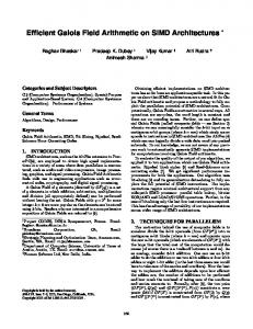
Future processors will likely use wider SIMD and a large number of CMP cores to exploit DLP and TLP [20]. In this section, we use the aforementioned analytical model and detailed simulation to study how changes in SIMD width and core count may affect MergeSort performance. First, we look at how varying SIMD width affect mergesort performance. In Section 5.2, we proposed an analytical model for our SIMD implementation and analyzed it for the parameters for today’s architecture. We now further analyze the model for other parameters. Recall from Section 5.2 that we use a, b and c to represent min/max latency, shuffle latency and inter-functional-unit latency, respectively. • (a = 1), (b = 1), and (c = 1): With the advancement in microarchitecture, it is reasonable to expect the

Speedup over 4-wide (3,1,1)

6.5 Performance on Future Platform

9 8 7 6 5 4 3 2 1 0

(3,1,1) (1,1,1) (1,1,0)

4

8

16 SIMD Width

32

64

Figure 9: Speedup as SIMD width increases from 4-wide to 64-wide for different latencies of (a, b, c).

4

Some of the missing numbers correspond to either the data not being available, or the input size being too big to fit in the Cell/GPU memory.

In Figure 9, we plot the speedup in execution time (in cycles per element per iteration) with varying SIMD width

for different values of a, b and c. The data size N is fixed at 16M elements. All numbers are plotted w.r.t. a 4-wide SIMD with (a, b, c)=(3,1,1). As evident from the graph, for any particular SIMD width, the speedup only varies by a few percent for different values of a, b and c. This is attributed to our scheduling algorithm that extracts the maximum performance for any given set of values for these parameters. In addition, the speedup increases near-linearly with the increase in SIMD width, and, in fact, is consistent with the O(N log(N ) log(2K)/K) running time of the algorithm. Next, we study how MergeSort would perform on a future CMP system and project performance for Intel’s upcoming Larrabee – a many-core x86 architecture with simple in-order cores and 512-bit SIMD instructions [20]. For our experiments, we use a cycle-accurate, execution-driven simulator of Larrabee architecture with an assumed frequency of 1GHz. Table 4 lists the projected runtimes for dataset sizes of 64M and 256M elements, with the number of cores varying from 8-32 cores. Our algorithm scales near-linearly on Larrabee, well beyond 32 cores. Number Of Elements 64M 256M

8C 0.636 2.742

16C 0.324 1.399

32C 0.174 0.751

Table 4: Projected performance (in seconds) on Larrabee architecture [20]. Additionally, we use the analytical model to study how changes in the cache size and the processor frequency would affect the performance. Cache size determines the block size that each thread uses to sort in the first phase, followed by the multiway merging during the second phase. The larger the cache size, the fewer the iterations in the second phase. Since each iteration of the second phase is only slightly expensive than in the first phase, doubling the cache size improves the execution time only by 2–3%. On the other hand, increasing the frequency of the processor will proportionately improve the overall performance, since the execution time per element per iteration (Tse and Tpe in the equations in Section 5) are proportionately reduced.

7. CONCLUSIONS We have presented an efficient implementation and detailed analysis of MergeSort on current CPU architectures. This implementation exploits salient architectural features of modern processors to deliver significant performance benefit. These features include cache blocking to minimize access latency, vectorizing for SIMD to increase compute density, partitioning work and load balancing among multiple cores, and multiway merging to eliminate the bandwidth bound stages for large input sizes. In addition, our implementation uses either wider sorting network or multiple independent networks to increase parallelism and hide backto-back instruction dependences. These optimizations enable us to sort 256M numbers in less than 2.5 seconds on a 4-core processor. We project near-linear scalability of our implementation with up to 64-wide SIMD, and well beyond 32 cores.

8. ACKNOWLEDGEMENTS We would like to thank Hiroshi Inoue for sharing the PowerPC performance numbers and Professor John Owens,

Mark Harris and Nadathur Rajagopalan Satish for providing the Nvidia GPU numbers. We are also thankful to Ronny Ronen for his comments on an initial version of the paper, and the anonymous reviewers for their insightful comments and suggestions.

9.

REFERENCES

[1] K. E. Batcher. Sorting networks and their applications. In Spring Joint Computer Conference, pages 307–314, 1968. [2] G. Bilardi and A. Nicolau. Adaptive bitonic sorting: an optimal parallel algorithm for shared-memory machines. SIAM J. Comput., 18(2):216–228, 1989. [3] Intel 64 and IA-32 architectures optimization reference manual. http://www.intel.com/products/processor/manuals. [4] M. V. de Wiel and H. Daer. Sort Performance Improvements in Oracle Database 10g Release2. An Oracle White Paper, 2005. [5] R. Francis and I. Mathieson. A Benchmark Parallel Sort for Shared Memory Multiprocessors. IEEE Transactions on Computers, 37:1619–1626, 1988. [6] R. S. Francis, I. D. Mathieson, and L. Pannan. A Fast, Simple Algorithm to Balance a Parallel Multiway Merge. In PARLE, pages 570–581, 1993. [7] B. Gedik, R. R. Bordawekar, and P. S. Yu. CellSort: High Performance Sorting on the Cell Processor. In VLDB ’07, pages 1286–1297, 2007. [8] N. Govindaraju, J. Gray, R. Kumar, and D. Manocha. GPUTeraSort: High Performance Graphics Co-processor Sorting for Large Database Management. In Proceedings of the ACM SIGMOD Conference, pages 325–336, 2006. [9] A. Greß and G. Zachmann. GPU-ABiSort: Optimal Parallel Sorting on Stream Architectures. In Proceedings of the 20th IEEE International Parallel and Distributed Processing Symposium, page 45, Apr. 2006. [10] M. Gschwind. Chip Multiprocessing and the Cell Broadband Engine. In CF ’06: Proceedings of the 3rd conference on Computing frontiers, pages 1–8, 2006. [11] H. Inoue, T. Moriyama, H. Komatsu, and T. Nakatani. AA-Sort: A New Parallel Sorting Algorithm for Multi-Core SIMD Processors. In PACT ’07, pages 189–198, 2007. [12] Intel Advanced Vector Extensions Programming Reference. http://softwarecommunity.intel.com/isn/downloads/intelavx/IntelAVX-Programming-Reference-31943302.pdf/,2008. [13] D. E. Knuth. The Art of Computer Programming, Volume 3: (2nd ed.) Sorting and Searching. 1998. [14] S. Lacey and R. Box. A Fast, Easy Sort. Byte Magazine, pages 315–320, 1991. [15] W. A. Martin. Sorting. ACM Comp Surv., 3(4):147–174, 1971. [16] T. Nakatani, S.-T. Huang, B. Arden, and S. Tripathi. K-way Bitonic Sort. IEEE Transactions on Computers, 38(2):283–288, Feb 1989. [17] R. Parikh. Accelerating QuickSort on the Intel Pentium 4 Processor with Hyper-Threading Technology. softwarecommunity.intel.com/articles/eng/2422.htm/, 2008. [18] T. J. Purcell, C. Donner, M. Cammarano, H. W. Jensen, and P. Hanrahan. Photon Mapping on Programmable Graphics Hardware. In Graphics Hardware 2003, pages 41–50, July 2003. [19] N. R. Satish, M. Harris, and M. Garland. Designing Efficient Sorting Algorithms for Manycore GPUs. Submitted to SuperComputing 2008. [20] L. Seiler, D. Carmean, E. Sprangle, T. Forsyth, M. Abrash, P. Dubey, S. Junkins, A. Lake, J. Sugerman, R. Cavin, R. Espasa, E. Grochowski, T. Juan, and P. Hanrahan. Larrabee: A Many-Core x86 Architecture for Visual Computing. Proceedings of SIGGRAPH, 27(3):to appear, 2008. [21] S. Sengupta, M. Harris, Y. Zhang, and J. D. Owens. Scan Primitives for GPU Computing. In Graphics Hardware 2007, pages 97–106, Aug. 2007. [22] E. Sintorn and U. Assarsson. Fast Parallel GPU-Sorting Using a Hybrid Algorithm. In Workshop on General Purpose Processing on Graphics Processing Units, 2007. [23] P. Tsigas and Y. Zhang. A Simple, Fast Parallel Implementation of Quicksort and its Performance Evaluation on SUN Enterprise 10000. pdp, 00:372, 2003. [24] S. Vangal, J. Howard, G. Ruhl, S. Dighe, H. Wilson, J. Tschanz, D. Finan, P. Iyer, A. Singh, T. Jacob, S. Jain, S. Venkataraman, Y. Hoskote, and N. Borkar. An 80-Tile 1.28TFLOPS Network-on-Chip in 65nm CMOS. In Proceedings of Solid-State Circuits Conference, pages 98–589, 2007.