Unité de Recherche Associée au Centre National de la Recherche Scientifique. No. 1793, Université Blaise Pascal Les Cézeaux, 63177 Aubi`ere Cedex, ...
G. Granet and B. Guizal
Vol. 13, No. 5 / May 1996 / J. Opt. Soc. Am. A
1019
Efficient implementation of the coupled-wave method for metallic lamellar gratings in TM polarization G. Granet ´ ecommunications, ´ Institut National des Tel 9 rue Charles Fourier, 91011 Evry Cedex, France
B. Guizal Laboratoire des Sciences, des Materiaux ´ pour l’Electronique et d’Automatique, Unite´ de Recherche Associ´ee au Centre National de la Recherche Scientifique No. 1793, Universite´ Blaise Pascal Les Cezeaux, ´ 63177 Aubiere ` Cedex, France Received December 7, 1995; accepted December 21, 1995 A new implementation of the coupled-wave method for TM polarization is proposed. We use a second-order differential operator established by Nevi`ere together with a scattering-matrix approach. Thus we obtain for metallic gratings a convergence rate as quick as that in TE polarization. 1996 Optical Society of America
1.
INTRODUCTION
In two recent papers1,2 Moharam et al. reviewed the coupled-wave method (CWM) for describing the diffraction of electromagnetic waves by periodic grating structures. By exploitation of the symmetry of the diffraction problem they derived a second-order wave equation for both TE and TM polarizations, which is a nice improvement over preceding formulations. They also proposed an enhanced transmittance matrix approach to overcome numerical difficulties that appear as the grating thickness is increased. However, as has already been reported and analyzed by Li and Haggans,3 the new formalism still exhibits a poor convergence rate especially for metallic gratings in TM polarization. Unlike these authors, we do not believe that the origin of this low convergence is the use of Fourier expansions for the permittivity and the electromagnetic field in the grating region, but rather lies in the formulation itself. Indeed the CWM belongs to the so-called differential methods, and its originality and novelty lie in the method of solution, which involves only elementary mathematics and numerical techniques such as the search for eigenvalues and eigenvectors. However, differential methods have been used for a long time by Nevi`ere4 and Vincent,5 and we propose, in this paper, an efficient implementation of the CWM for TM polarization based on the second-order differential operator that they presented many years ago. As a result, there is no noticeable difference between the convergence rate for the two polarizations for metallic gratings. The second step of the CWM consists of matching the tangential components of the field at the interfaces of the grating. For this purpose we use a scattering-matrix approach, which is an alternative to the enhanced transmittance approach of Moharam et al. and to the characteristic matrix formalism of Chateau and Hugonin.6 However, it should be noted that this point is not at all responsible for the good convergence obtained. 0740-3232/96/051019-05$10.00
Since much has been said about it, the reader is assumed to be familiar with the mathematical formulations of the CWM. The goal of this paper is to remove a deficiency of the CWM with respect to metallic gratings in TM polarization. To show the efficiency of our implementation we will compare our results with those that would be obtained with use of the implementation of Moharam et al.
2.
FORMULATION
The grating diffraction configuration is depicted in Fig. 1. A linear polarized electromagnetic wave with transverse magnetic polarization is obliquely incident on a lamellar grating. Region 1 (the input region) is a homogeneous dielectric with a relative permittivity of e1 . Similarly, region 3 is homogeneous with a relative permittivity of e3 . Region 2 is the grating region. It consists of a periodic distribution of both types of material: ( e3 if 0 , x , fd , e2 sxd (1) e1 if fd , x , d where f denotes the fill factor, i.e., the fraction of the grating period occupied by the region of permittivity e3 . The permittivity in this region may be expressed in a Fourier series as ! √ X 2pp x , (2) e2 sxd e2p exp 2i d p and its inverse as ! √ X 1 2pp x . e˜2p exp 2i e2 sxd d p
(3)
We denote by l the wavelength in free space by k its corresponding wave number. A time dependence of the form expsivtd is assumed. 1996 Optical Society of America
1020
J. Opt. Soc. Am. A / Vol. 13, No. 5 / May 1996
G. Granet and B. Guizal
≠ ≠x
"
1 ≠H2z k2 e2 sxd ≠x
#
≠ 1 ≠y
"
1 ≠H2z k2 e2 sxd ≠y
# 1 H2z 0 . (10)
Fig. 1. Geometry for the lamellar metallic grating analyzed herein.
It should be noted that even if k2 e2 sxd is discontinuous, fk2 e2 sxdg21 = H2z exhibits a continuous normal derivative. This property implies that we should never split the products sk2 e2 d21 ≠H2zy≠y and sk2 e2 d21 ≠H2zy≠x. Projecting on the exps2ikam xd basis with H2zm s yd, the components of H2z , we obtain X ap e˜2 m-p H2zp s yd 2 H2zm s yd am p
In regions 1 and 3 the tangential components of the electromagnetic field may be expressed as: In region 1, Ω ∑ P P 11 A1 q dmq exps2ikb11q yd H1 z s y, xd m q ∏æ P 2 1 A21 d exps2ikb yd 1 q mq 1q
≠2 1 X e˜2 m-p fH2zp s ydg . (11) 2 k p ≠y 2
The above set of coupled-wave equations should be solved by calculation of the eigenvalues and eigenvectors associated with the following N 3 N T matrix: ˜ , T feg ˜ 21 sI 2 fagfegfagd
(12)
q
3 exps2ikam xd , Ω ∑ P 11 P E1 x s y, xd ikb11q A1 q dmq exps2ikb11q yd m q ∏æ P 2 1 ikb12q A21 1 q dmq exps2ikb1 q yd
(4)
q
(5)
3 exps2ikam xd .
where N is the truncation number, i.e., the number of harmonics retained in the field expansion, I is the unity matrix, a is a diagonal matrix with diagonal elements am , and feg and feg ˜ are matrices with their m, pth element equal to e2,m-p and e˜2,m-p , respectively, defined in Eqs. (2) and (3). However, better numerical results are obtained with a slightly different matrix:
In region 3, H3 z s y, xd
√ Ω P P
T 0 feg ˜ 21 sI 2 fagfeg21 fagd . A12 3 q dmq
expf2ikb31q s y
1 hdg æ∂ P 2 1 A22 d expf2ikb s y 1 hdg mq 3q 3q m
q
Indeed, from Eqs. (2) and (3) we can deduce the matrix relation feg` feg ˜ ` I,
q
3 exps2ikam xd , (6) √ Ω P P 1 E3 x s y, xd ikb31q A12 3 q dmq expf2ikb3 q s y 1 hdg m q æ∂ P 2 1 ikb32q A22 d expf2ikb s y 1 hdg mq 3q 3q q
(7)
3 exps2ikam xd , where ( dmq 1 bjq
1 0
2 2bjq
if m q , if m fi q v !2 √ u u l t ej 2 sin u 1 q and d
and l . d
which is true only for the untruncated matrices feg` and feg ˜ ` . Nevertheless, assuming that the above relation is still valid for the truncated matrices, we replace feg ˜ with the inverse of feg in Eq. (12). Moharam et al. probably arrived at the same conclusion about the choice of feg21 rather than feg, ˜ but they do not say so explicitly. Indeed, Eq. (35) of Ref. 1 is not deduced directly from Eqs. (30) – (33). If such were the case, it should be written as ˜ . T 00 fegsI 2 fagfegfagd
1 1 Resbjq d 2 Imsbjq d . 0 (8)
aq sin u 1 q
(13)
(9)
The superscripts 1 and 2 in the amplitude coefficients A61 1q and A62 3q refer to the upper face (first interface) and the lower face (second interface), respectively. In region 2 the z component of the magnetic field satisfies the following equation:
(14)
So the fundamental difference between our implementation and theirs lies in the fact that we replace feg ˜ 21 with feg. Finally, the tangential component of the magnetic field in region 2 is given by Ω ∑ P P 1 1 A2 q H2z mq exps2ikrq1 yd H2 z m q ∏æ P 2 2 H exps2ikr yd exps2ikam xd , 1 A2 2 q 2z mq q q
(15) where rq1 and rq2 are the square roots of the eigenvalues rq2 of the T matrix defined as
G. Granet and B. Guizal
Vol. 13, No. 5 / May 1996 / J. Opt. Soc. Am. A
8q > 2 > > < q rq 1 2 rq 2rq rq2 > > > :
if rq2 is real
H2 z s y 2hd
,
with negative imaginary part if rq2 is complex (16) 1 2 and where H2z mq and H2z mq are elements of the associated 2 eigenvector matrices H1 2z and H2z . The tangential electric field is related to the tangential magnetic field by E2x
1 ≠H2z . ive2 ≠y
q
(18)
We define two matrices
E1 2x ,
E2 2x
as
1 1 1 E2x fegfH ˜ 2z gfr g 2 E2x
(19)
2 2 fegfH ˜ 2z gfr g ,
(20)
where fr1 g and fr2 g are diagonal matrices with diagonal elements rq1 and rq2 .
m
q
3 exps2ikam xd ,
q
(21)
∏æ
2 2 A22 2 q H2z mq expsikrq hd
(22)
At the boundary between the input region and region 2, matching the tangential components of the field leads to "
A111 A221
#
" S
1
A121 A211
# ,
(23)
with "
I S 1 E1x 1
2I 2E2 1x
#21 "
2H2 2z 2E2 2x
1 H2z E1 2x
# ,
(24)
and at the boundary between region 2 and the output region " # " # 22 A212 2 A2 , S (25) A322 A312 with "
1 H2z S 1 E2x
SCATTERING-MATRIX APPROACH
The second step in the CWM is the resolution of a linear system deduced from the boundary matching conditions, which can be analyzed by the S-matrix concept widely used in microwave circuit theory. This formalism has already been used by Cotter et al.7 for layers with parallel modulated faces and by Granet et al.8 for layers with no parallel faces. Since eigenvalues are deduced from their squared number, there will be two sets of modes: those propagating or decaying in the positive y direction and those traveling in the opposite direction, which we have referred to with a superscript plus and minus, respectively. The scattering matrix couples the tangential components of the incoming waves with the same components of the outgoing waves. Hence each face of a layer may be assimilated to a 2N port network, with N the truncation number. In region 2 it is useful to express the phase of the field in relation to the upper face and the lower face. For that purpose we introduce four am21 12 22 plitude vectors whose elements are A11 2 q , A2 q , A2 q , A2 q , where the superscripts 1 and 2 refer to the upper face (first interface) and the lower face (second interface), respectively. The layer itself is then supposed to interconnect N ports of each junction. This model is depicted schematically in Fig. 2. Relation 15, when applied to y 0 and then to y 2h, gives ∑ µ ∂∏ P P 11 1 P 2 H2 z s y 0d A2 q H2z mq 1 A21 H 2 q 2z mq
P
1 1 A12 2 q H2z mq expsirq hd
3 exps2ikam xd .
2
3.
q
q
l
3 exps2ikam xd .
m
1
(17)
Substituting the expansion of Eq. (15) into Eq. (17), we obtain ∑ P P P 1 1 2ikrq1 A1 e˜l H2z E2 x 2q m-lq exps2ikrq yd m q l ∏ P P 2 2 1 ikrq2 A2 e ˜ H exps2ikr yd l 2z m-lq 2q q
Ω ∑ P P
1021
2 2H2z 2 2E2x
#21 "
I E1 3x
2I 2 2E3x
# .
(26)
In region 2 the scattered waves from the upper face are the incident waves on the lower one. This is modeled by a third S matrix, which is antidiagonal: " # " # A11 A221 2 S 12 A222 A212
(27)
with "
S1 2
0 f2
f2 0
# ,
(28)
where f2 is a diagonal matrix with diagonal elements expsikrq1 hd. The global S matrix is obtained by classical recursion
Fig. 2. tion.
Scattering by a lamellar grating and S-matrix formula-
1022
J. Opt. Soc. Am. A / Vol. 13, No. 5 / May 1996
G. Granet and B. Guizal
formulas, and Eqs. (23), (25), and (27) become # " # " A121 . A111 S A322 A312
(29)
Vector A312 is null because there is no incident wave on the structure from region 3, and A121 has only one nonzero component corresponding to the incident wave. Therefore the 2N unknown values of A111 and A322 can be calculated. The reflected efficiencies are given by 2 eq jA11 1q j
4.
b11q . cos u
(30)
NUMERICAL RESULTS
We consider the case from the previously mentioned paper by Li and Haggans.3 It consists of a lamellar grating with a groove depth of 1 mm. The dielectric has an p optical index of e3 0.22 2 i6.71. The incident wavelength l, the period d, and the height h of the grating are 1 mm. The angle of incidence is equal to 30±. Figure 3 shows the convergence of the diffraction efficiencies in TM polarization as the truncation order increases for our implementation and for that of Moharam et al. It can be seen that the efficiencies computed with our program converge remarkably fast. Table 1 lists the numerical values of the TM diffraction efficiencies computed with our implementation for different truncation orders and different groove depths. They are compared with assumed exact values that have been calculated with the modal method by modal expansion and the well-known R-matrix approach. It can be seen that our implementation, which uses the new eigenvalue formulation and the S-matrix approach, can deal with deep gratings. Fig. 3. Convergence of (a) the negative first-order and (b) the zeroth-order diffraction efficiencies for TM polarization computed with our implementation (circles) and with the implementation of Moharam et al. (crosses).
Table 1. Numerical Values of TM Diffraction Efficiencies Computed at Three Different Truncation Orders And for Three Different Groove Depths Truncation Order
Diffraction Efficiencies e21
e0
h 0.1 N 41 N 81 N 121 Exact
0.3389 0.3408 0.3404 0.3408
0.6282 0.6289 0.6301 0.6312
h1 N 41 N 81 N 121 Exact
0.1015 0.1015 0.1015 0.1024
0.8425 0.847 0.8474 0.8477
h 4.8 N 41 N 81 N 121 Exact
0.0445 0.0493 0.0499 0.0503
0.5142 0.5009 0.4995 0.4985
5.
CONCLUSION
In this paper we have proposed an implementation of the CWM for TM polarization based on a rigorous formulation by Nevi`ere. Furthermore, we have expressed the boundary conditions with the S-matrix approach. We have shown that the resulting implementation overcomes the difficulties of the implementation of Moharam et al. for metallic gratings, so it should be useful for those who use the CWM.
ACKNOWLEDGMENT The authors are grateful to Lifeng Li for providing them the assumed exact values of Table 1.
REFERENCES 1. M. G. Moharam, Eric B. Grann, Drew A. Pommet, and T. K. Gaylord, “Formulation for stable and efficient implementation of the rigorous coupled-wave analysis of binary gratings,” J. Opt. Soc. Am. 12, 1068 – 1076 (1995). 2. M. G. Moharam, Eric B. Grann, Drew A. Pommet, and T. K. Gaylord, “Stable implementation of the rigorous coupledwave analysis for surface-relief gratings: enhanced transmittance matrix approach,” J. Opt. Soc. Am. 12, 1077 – 1086 (1995). 3. Lifeng Li and Charles W. Haggans, “Convergence of the coupled-wave method for metallic lamellar diffraction gratings,” J. Opt. Soc. Am. 10, 1184 – 1189 (1993).
G. Granet and B. Guizal 4. M. Nevi`ere, “Sur un formalisme diff´erentiel pour less probl`emes de diffraction dans le domain de r´esonance: application a` l’´etude des r´eseaux optiques et de diverses structures p´eriodiques,” th`ese de doctorat (Universit´e d’Aix – Marseille, Aix – Marseille, France, 1975). 5. P. Vincent, “Differential methods,” in Electromagnetic Theory of Gratings, R. Petit, ed. (Springer – Verlag, Berlin, 1980), Chap. 4. 6. Nicolas Chateau and Jean-Paul Hugonin, “Algorithm for
Vol. 13, No. 5 / May 1996 / J. Opt. Soc. Am. A
1023
the rigorous coupled-wave analysis of grating diffraction,” J. Opt. Soc. Am 11, 1321 – 1331 (1994). 7. N. P. K. Cotter, T. W. Preist, and J. R. Sambles, “Scatteringmatrix approach to multilayer diffraction,” J. Opt. Soc. Am. 12, 1097 – 1103 (1995). 8. G. Granet, J. P. Plumey, and J. Chandezon, “Scattering by a periodically corrugated dielectric layer with non-identical faces,” Pure Appl. Opt. 4, 1 – 5 (1995).