Efficient Joint Maximum-Likelihood Channel ...

Efficient Joint Maximum-Likelihood Channel Estimation and Signal Detection H. Vikalo‡ , B. Hassibi‡, and P. Stoica§

Abstract In wireless communication systems, channel state information is often assumed to be available at the receiver. Traditionally, a training sequence is used to obtain the estimate of the channel. Alternatively, the channel can be identified using known properties of the transmitted signal. However, the computational effort required to find the joint ML solution to the symbol detection and channel estimation problem increases exponentially with the dimension of the problem. To significantly reduce this computational effort, we formulate the joint ML estimation and detection as an integer least-squares problem, and show that it can be solved via sphere decoding in polynomial expected time. Index Terms—Integer least-squares problem, sphere decoding, wireless communications, multipleantenna systems, lattice problems, NP hard, expected complexity, joint detection and estimation

‡

(hvikalo,hassibi)@systems.caltech.edu; California Institute of Technology, Pasadena, CA 91125 This work was supported in part by the NSF under grant no. CCR-0133818, by the Office of Naval Research under grant no. N00014-02-1-0578, and by Caltech’s Lee Center for Advanced Networking. § Uppsala University, Department of Systems and Control, Uppsala, Sweden

1 Introduction The pursuit for high-speed data services has resulted in a tremendous amount of research activity in the wireless communications community. To obtain high reliability of the transmission, particular attention has been payed to the design of receivers (see, e.g., [1] and references therein). In the system design, one often assumes knowledge of the channel coefficients at the receiver. These are typically obtained by sending a training sequence, thus sacrificing a fraction of the transmission rate. On the other hand, in practical systems, due to rapid changes of the channel and/or limited resources, training and channel tracking may be infeasible. One possible remedy is to differentially encode the transmitted data and thus eliminate the need for the channel knowledge. Another one is to exploit known properties of the transmitted data to learn the channel blindly – for instance, one can exploit the fact that the transmitted data belongs to a finite alphabet. We consider a problem of joint maximum-likelihood (ML) channel estimation and signal detection in a communication system where the transmitters use only one antenna but the receiver employs multiple antennas. This can, for instance, be the case on an uplink, where all users (transmitters) have a single antenna, while the base station (receiver) has multiple antennas. Let N denotes the number of receive antennas and let T be the time interval during which the channel coefficients remains constant and change to an independent set of values afterwards (i.e., we assume the block-fading channel model). The received signal can be written as

∗

X = HS + W = H

where H =



h 1 h2 . . . hM





Sτ∗

Sd∗



+ W,

(1)

is the N × M channel matrix comprised of N single-input

multi-output (SIMO) channel gain vectors hi , i = 1, 2, . . . , M , whose entries are independent, identically distributed (iid) complex Gaussian random variables CN (0, 1). Matrix S τ is the (deterministic and known) Tτ × M matrix of training symbols, while the matrix Sd is Td × M matrix of

2

data symbols, and where T = Tτ + Td . We assume that all elements of Sτ and Sd are unitary, i.e., 2 |sij τ | = 1, 1 ≤ i ≤ Tτ , 1 ≤ j ≤ M, 2 |sij d|

(2)

= 1, 1 ≤ i ≤ Td , 1 ≤ j ≤ M,

ij where sij τ denotes an (i, j) entry in Sτ , and where sd denotes an (i, j) entry in Sd . Furthermore,

N × T matrix W is an additive noise matrix whose elements are assumed to be iid complex Gaussian random variables C(0, σ 2 ). The joint ML channel estimation and signal detection problem can be stated as follows:

min kX − HS ∗ k2 , H,S

(3)

where the entries of S satisfy (2). Problem (3) is a mixed optimization problem: it is a leastsquares problem in H and an integer least-squares problem in S. Traditionally, the solution to the integer least-squares problems is found by an exhaustive search over the entire symbol space. The complexity of exhaustive search is exponential in M Td and often infeasible in practice. Therefore, low-complexity heuristic techniques, usually iterating between the S and the estimate of H, are often employed (see, e.g., [2] and the references therein). On the other hand, in communication applications, the sphere decoding [3] is recognized as a technique for solving integer least-squares problems at polynomial expected complexity [4, 5]. In this paper, we show how the sphere decoding algorithm can be employed to find the solution of (3), and prove that, at high SNR, the expected complexity results of [4, 5] hold. In other words, we show that the joint ML channel estimation and symbol detection problem (3) can be solved in polynomial expected time over a wide range of system parameters. We should remark that the basic sphere decoding algorithm performs the closest point search in a rectangular lattice and the available expected complexity results assume the same. Therefore, when discussing complexity, we will assume that the entries of S belongs to a QPSK constellation (so that (2) hold). However, 3

sphere decoding can easily be modified and used for detection of symbols coming from a PSKmodulation schemes [6]. Note that the model (1) include both the blind and the training-based scheme – blind scheme model is obtained by simply setting Tτ = 0. In this paper, we consider both schemes. We start by considering single user system (M = 1), for which we solve (3) for both T τ = 0 and Tτ > 0. This is presented in Section 2, while Section 3 contains generalization of the T τ > 0 case to the multi-user scenario. We discuss only training-based multi-user case in order to avoid ambiguities that arise in blind scenarios. An interesting result of Section 3 implies that the complexity of the algorithm grows only linearly with the number of users. The complexity of the sphere decoding algorithm for solving (3) is discussed in Section 3, and the results therein imply polynomial expected complexity of the algorithm over a wide range of system parameters. In Section 5, we briefly discuss use of soft sphere decoding for joint detection and decoding in systems employing channel codes. Simulation results are presented in Section 6, while the summary and conclusion are in Section 7.

2 Single user case We consider a single-user case, i.e., consider the model (1) for M = 1. Then the received signal can be written as ∗

X = hs + W = h



s∗τ

s∗d



+ W,

(4)

and the optimization problem that needs to be solved is

min kX − hs∗ k2 , h,s

(5)

where the entries of s have unit power. The blind and the training-based schemes for solving (5) are treated in the remainder of this section. 4

2.1 Blind joint ML estimation and detection Assuming that there is no training sequence (Tτ = 0), so that sd = s and the model (4) becomes

X = hs∗ + W = hs∗d + W.

(6)

ˆ that minimizes (6) is given by For any given s, the channel h ˆ = Xs/ksk2 = 1 Xs, h T

(7)

where we used the assumption that the entries of s have unit power. Substituting (7) in (5) gives 1 ∗ 2 ss )k T 1 = tr [X(I − ss∗ )X ∗ ] T 1 = tr (XX ∗ ) − s∗ X ∗ Xs T

kX − hs∗ k2 = kX(I −

(8)

Hence the optimization (5) is equivalent to solving

max s∗ X ∗ Xs. s

(9)

Optimization problem (9) is over vectors s with integer values and a straightforward way to solve it is via exhaustive search [2]. On the other hand, the sphere decoding algorithm efficiently solves optimization problems over integers. However, the sphere decoding problem minimizes objective function over integer-valued vectors, and thus we need to express (9) accordingly. To this end, let ˆ = λmax (X ∗ X) denote the maximum eigenvalue of X ∗ X, and let ρ > λ ˆ (for instance, we can λ choose ρ = tr(X ∗ X)). The problem (9) is then equivalent to

min s∗ (ρI − X ∗ X)s. s

5

(10)

The optimization problem (10) is an integer least-squares problem. Furthermore, note that due to the choice of ρ, the matrix (ρI − X ∗ X) is positive definite and therefore it allows for the Cholesky factorization of the form ρI − X ∗ X = R∗ R,

(11)

where R is an upper-triangular matrix. Thus the sphere decoding algorithm of Fincke and Pohst [3] can be applied to solve (10). Rather than exhaustively searching over the entire symbol space, the sphere decoding algorithm performs a limited search inside a sphere of an appropriately chosen radius r, i.e., finds the point sd that minimizes (10) among all lattice points that satisfy

s∗ X ∗ Xs ≤ r 2 .

(12)

(The choice of the radius r in (12) will be discussed in Section 4.) The closest lattice point to the origin inside the sphere is the solution to (10). The sphere decoding algorithm breaks down condition (12) into a set of T necessary conditions that the components of the vector s need to satisfy. The algorithm can be related to nulling and canceling (see, e.g., [7]) where, after a component of the vector s that satisfies (12) is found, its contribution to s∗ X ∗ Xs is subtracted. However, unlike in nulling and canceling, in sphere decoding the components of s are not fixed until an entire vector s which satisfies (12) is found. We omit any further details for brevity and refer the interested reader to [3], or to [4, 5] and the references therein. Furthermore, for an application of complex sphere decoding, relevant for detection of symbols coming from PSK constellations, we refer the reader to [6]. Finally, we should remark that the sphere decoding algorithm can be interpreted as a tree search procedure, as illustrated in Figure 1, where the nodes on the k th level of the tree correspond to kdimensional subvectors sk of the unknown vector s. We will find this tree-search interpretation useful when later discussing training-based schemes.

6

2.2 Joint ML estimation and detection in training-based schemes Assume that Tτ > 0, i.e., training sequence sτ preceeds the data block sd . The optimization problem (10) can then be written as

min sd



s∗τ s∗d







 sτ  (ρI − X ∗ X)  . sd

(13)

For simplicity, we will find it useful to define

ρI − X ∗ X = Γ. Recall that we choose ρ such that ρ > λmax (X ∗ X). Therefore, matrix Γ is positive definite. Partition Γ as





 Γ11 Γ12  Γ= , ∗ Γ12 Γ22 and note that, since Γ is positive definite, so is Γ2 . Therefore, we can write 

s∗τ s∗d









 Γ11 Γ12   sτ  ∗ ∗ ∗ ∗ ∗  = sτ Γ11 sτ + sτ Γ12 s + sd Γ12 sτ + sd Γ22 sd   sd Γ∗12 Γ22

∗ ∗ −1 ∗ ∗ = (sd − Γ−1 22 Γ12 sτ ) Γ22 (sd − Γ22 Γ12 sτ ) + sτ Γ11 sτ

Since s∗τ Γ11 sτ does not depend on sd , the optimization (13) becomes ∗ ∗ −1 ∗ −1 ∗ 2 min(sd − Γ−1 22 Γ12 sτ ) Γ22 (sd − Γ22 Γ12 sτ ) = min ksd − Γ22 Γ12 sτ kΓ22 , sd

sd

which we can solve with the sphere decoding algorithm.

7

3 Multi-user case We now focus on the general multi-user case. The relevant optimization problem is the one (3). For any S, optimal channel estimate H is obtained as ˆ = XS(S ∗ S)−1 S ∗ , H

and thus we have

arg min kX − HS ∗ k2 = arg min kX − XS(S ∗ S)−1 S ∗ k2 H,S

S

= arg min tr {X(I − S(S ∗ S)−1 S ∗ )X ∗ } S

= arg max tr {(S ∗ S)−1 S ∗ X ∗ XS} S

Recall that S is comprissed of unitary symbols. If the users are uncorrelated, then S ∗ S ≈ T I, and it follows that

∗

−1

∗

∗

arg max tr {(S S) S X XS} = arg max S

s1 ,...,sM

M X

(sk )∗ (X ∗ X)sk ,

k=1

where sk is the symbol vector of the k th user (i.e., the k th row in matrix S). Furthermore,

max

M X

k ∗

∗

k

(s ) (X X)s = min

s1 ,...,sM

k=1

M X k=1

(sk )∗ (ρI − X ∗ X)sk ,

and thus, since the users choose their signals independently, optimization (3) is equivalent to the optimization problem min(sk )∗ (ρI − X ∗ X)sk , sk

k = 1, . . . , M.

(14)

From (14), it is clear that without knowing anything about the users, we could not resolve their signal vectors. Therefore, we insist on Tτ > 0, i.e., we assume training matrix Sτ with distinct 8

rows. This resolves user ambiguity. More intrestingly, optimization (14) implies that in order to detect signals received from M users, we only need to find M points inside the T -dimensional sphere – therefore, the dimension of the problem does not increase with the number of users, as one may expect. As a result, computational complexity grows only linearly in the number of users. 1 To explain how the sphere decoding is employed in this case, recall the tree-search interpretation of the algorithm discussed in Section 2.1. We search for M vectors s k , 1 ≤ k ≤ M , in T -dimensional sphere of radius r. Each such vector allows for partition of form 

 sk = 

skτ skd



 ,

where skτ is known to the receiver. In fact, matrix Sτ is comprised of all such vectors skτ . For each skτ , the sphere decoding algorithm then performs search for sk minimizing (14). One can interpret the search for sk as a tree-search procedure where the root of the tree is fixed to skτ . This is illustrated in Figure 2. Note that by insisting on Tτ > 0, we sacrifice some rate. However, this is typically required in order to resolve user ambiguity. Once this ambiguity is gone, sphere decoding can be employed with no additional requirements on the structure of transmitted data.

4 Complexity of the algorithm and choice of the search radius Choice of the search radius is crucial for the computational complexity of the sphere decoding algorithm. If the radius is too small, we may not find anything and thus may have to repeat the search with larger radius. On the other hand, if the radius is too big, the algorithm has to go through many points which requires significant computation time. 1

Actually, increase in the computational complexity is even less than linear in the number of users. The reason for that is in the fact that preprocessing – i.e., finding ρ and performing the QR-factorization of (ρI − X∗ X) – needs to be done only once for all users.

9

A simple choice of the radius could be based on the heuristic solutions to (3). For instance, an obvious heuristic for solving (3) consists of finding the eigenvector corresponding to the maximum eigenvalue of X ∗ X (or, equivalently, the dominant right singular vector of X) and then projecting it onto symbol space (i.e., rounding each entry). This heuristic can be exploited as a starting point of the sphere decoding search – the norm of the heuristic solution can be used as the search radius. However, we cannot say much about the complexity of the sphere decoding algorithm for this deterministic choice of the search radius. Alternatively, when the distribution of the objective function of the minimization is known, one can choose radius according to some parameters of that distribution. For instance, in [4], objective function of the minimization problem that is being solved by sphere decoding has chisquare distribution, and the search radius is chosen according to the variance of that distribution. In particular, the variance is scaled in such a way that the probability of finding a point inside the sphere is very high. Furthermore, the expected complexity of the sphere decoding algorithm for such a choice of the radius is found and shown to be polynomial over a wide range of SNRs. In this section, we show next that the objective function in (10) has a chi-square distribution at high SNRs. Parameters of the distribution suggest a probabilistic choice of the search radius, while the expected complexity results of [4, 5] imply practical feasibility of the sphere decoding algorithm employed for solving (10). We start by proving the following lemma. Lemma 1. At high SNR, s∗ (ρI − X ∗ X)s is chi-square distributed. Proof: Assume large SN R, i.e., SN R  1. Consider the eigenvalue decomposition of X ∗ X,

X ∗X =



ˆ ˆ G u









ˆ ˆ   λ 0  u   , ˆ ˆ∗ 0 Λ G ∗

ˆ denotes the largest eigenvalue, and where diagonal elements of Λ ˆ are the remaining T − where λ ˆ we can write the objective function of the 1 eigenvalues in decreasing order. Taking ρ = λ, 10

minimization (10) as ˆ −u ˆ−G ˆΛ ˆG ˆ ∗ )s ˆu ˆ ∗λ s∗ (ρI − X ∗ X)s = s∗ (λI ˆ −u ˆΛ ˆG ˆ ∗ ]s ˆu ˆ∗) − G = s∗ [λ(I ˆ − Λ) ˆ λI ˆ G ˆ ∗s = s∗ G(

(15)

ˆG ˆ ∗ . Furthermore, ˆu ˆ∗ = G where in going from the second to the third line above, we used I − u X ∗ X = (X − hs∗ )∗ (X − hs∗ ) = khk2 ss∗ + sh∗ W + W ∗ hs∗ + W ∗ W

(16)

ˆ uuˆ∗ + G ˆΛ ˆG ˆ∗ = λˆ

(17)

On the other hand, for σ 2  1 (i.e., SN R  1), ∗

2

X X = khk T



s √ T



s∗ √ T



,

ˆ and Λ ˆ become and hence, at high SNRs, the theoretical values of λ

λ = T khk2 ,

Λ = 0.

(18)

Note that, using (16), we obtain ˆ ∗ (X ∗ X)s = G ˆ ∗ (khk2 ss∗ + sh∗ W + W ∗ hs∗ + W ∗ W )s G ˆ ∗ s) + (G ˆ ∗ s)h∗ W s + G ˆ ∗ W ∗ hT + G ˆ ∗W ∗W s = λ(G

11

(19)

On the other hand, from (17), ˆG ˆ∗G ˆΛ ˆG ˆ ∗ s = Λ( ˆ G ˆ ∗ s) ˆ ∗ (X ∗ X)s = λ ˆ ∗u ˆ ∗ + |{z} ˆu G G |{z} =0

(20)

=I

Combining (19) and (20) leads to

ˆ ∗ s) + (G ˆ ∗ s)h∗ W s + G ˆ ∗ W ∗ hT + G ˆ ∗ W ∗ W s = Λ( ˆ G ˆ ∗ s), λ(G

from which, letting σ 2 → 0 and neglecting higher order terms (those whose power goes as σ 4 ), we obtain ˆ ∗ s) + G ˆ ∗ W ∗ hT ≈ 0 ⇒ λ(G ˆ ∗ s) ≈ −G ˆ ∗ W ∗ hT, λ(G ˆ ∗ s) ≈ −G∗ W ∗ hT . Therefore, for high SNRs, which, since σ 2  1, we can further write as λ(G ˆ ∗ s) is circular Gaussian with zero mean. To find its variance, note that (G 

  TG W h = TG    ∗

∗

W1∗ h .. .

∗

WN∗ h



  ,  

where Wk denotes the k th column of W . Also, note that

E [Wk∗ hh∗ Wl ] = E [h∗ Wl Wk∗ h] = σ 2 khk2 δk,l , ˆ ∗ s covariance matrix is given by and thus G T2 cov(G∗ W ∗ h) λ2 T T2 khk2 σ 2 I = σ 2 I = 2 λ λ

ˆ ∗ s) = cov(G

= T σ 2 (λI − Λ)−1 , 12

where Λ = 0 was inserted for convenience. Therefore,   ˆ ∗ s) ∼ CN 0, T σ 2 (λI − Λ)−1 . (G ˆ Λ ≈ Λ, ˆ and therefore approximately At high SNR, λ ≈ λ, i h ∗ 2 ˆ −1 ˆ ˆ , (G s) ∼ CN 0, T σ ˆ (λI − Λ) where σ ˆ 2 is an estimate of σ 2 . This estimate can be obtained (see, e.g., [8] and the references therein) as the mean of the (N − 1) smallest eigenvalues of XX ∗ (or, alternatively, the smallest (N − 1) non-zero eigenvalues of X ∗ X). Therefore, we have just shown that the scaled term in (15), square distributed with (T − 1) degrees of freedom, and so is

1 ˆ ˆ λI (s∗ G)( Tσ ˆ2

1 s∗ (ρI Tσ ˆ2

ˆ G ˆ ∗ s), is chi− Λ)(

− X ∗ X)s.

We use the result of Lemma 1 to choose the size of the search radius for sphere decoding: 1. Single-user case, blind scheme: Recall that the probability density function of chi-square distribution is given by an incomplete gamma function. Therefore, we can choose the search radius r 2 = αT σˆ2 so that the cumulative density function Z

αT 0

γ(λ, T − 1)dλ = 1 − ,

(21)

where γ(·, ·) denotes an incomplete gamma function and 1 −  is set close to 1, say, 0.99. This means that the optimal point is inside the sphere with probabality 1 − . If the algorithm does not find any point inside the sphere, new radius needs to be calculated (say, by setting 1 −  = 0.999). 13

2. Single-user case, training-based scheme: Denoting the above computed radius for the blind scheme by r b , the radius for the trainingbased scheme, rt , may be chosen as

∗ rt2 = rb2 − s∗τ (Γ11 − Γ12 Γ−1 22 Γ12 )sτ .

ˆ Therefore, to prevent any possible numerical We should further remark that |R| = 0 for ρ = λ. ˆ as stated in Section 2. Then the search radius should be problems, we suggest choice ρ > λ, modified and it may be chosen as ˆ + r, r 0 = (ρ − λ) where r is chosen as implied by (21).

5 Soft decoding of channel codes and other remarks So far, we have assumed that the users send uncoded data. On the other hand, if the users employ channel codes, we can use sphere decoding techniques for soft iterative decoding. To this end, one can use modified sphere decoding (the FP-MAP algorithm) proposed in [13], or the list sphere decoding proposed in [6]. Both modifications exploit the fact that sphere decoding finds all points that satisfy sphere constaint, e.g., in the single-user case, finds all vectors s such that

kX − hsk2 ≤ r 2 . (For the FP-MAP algorithm, the condition is kX − hsk2 ≤ r 2 +

P

log p(si ), where p(si ) is the

a priori information about the ith component of s.) By an appropriate choice of the radius, one can guarantee that the algorithm will return a number of points, which are then used to for a soft 14

decision about the components of the vector s. Assuming that transmitter, prior to modulation, employs channel codes (such as convolutional, turbo, LDPC, etc.), the soft decisions made by the modified sphere decoder are then iterated with the soft decisions made by the channel decoder. For brevity, we refrain ourselves from a more detailed discussion and refer the reader to [6], [13]. On another note, in this paper we have been primarily concerned with posing the problem of the joint ML channel estimation and signal detection in a form to which sphere decoding can be applied, and establishing relation with the existing analytical treatment of the complexity of sphere decoding. There are many practical realizations of sphere decoding that perform even better. For instance, the Schnorr-Euchner version of sphere decoding presented in [10], and further analyzed in [11], the radius scheduling suboptimal scheme introduced in [12], etc. Applying those techniques to further lower the complexity of sphere decoding in the context of joint ML estimation and detection are highly desirable.

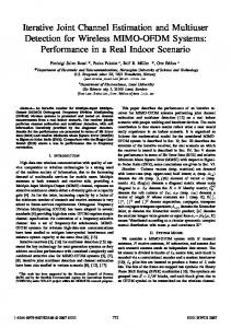
6 Simulation results In this section, we give several examples that illustrate the performace and the corresponding complexity of the sphere decoding algorithm in the previously described scenarios. Example 1 [Single-user system]: Consider a single user which employs one antenna, while the receiver employs N = 4 antennas. The data is transmitted in blocks of length T = 20. We compare the BER performance of the sphere decoding algorithm and the iterative least squares with projections (ILSP) algorithm (see, e.g., [2], [9]). [Simulation results are obtained by performing Monte Carlo runs in which h and W are varied.] The ILSP essentially finds the least squares estimate of the symbols and projects it onto the symbol space to obtain the estimate ˆs. Then ˆs is used to update the estimate of the channel and the two aforementioned steps repeated until convergence. As shown in Figure 2, the sphere decoding algorithm significantly outperforms ILSP over the

15

considered range of SNR. Figure 3 shows the complexity exponent, defined as

e = logT F,

where F denotes the total number of operations required to detect a vector s. (For the sphere decoding, the total complexity is a sum of the operations for the QR factorization and the sphere decoding search). It is evident that the sphere decoding has roughly cubic complexity over the range of SNRs of interest. Example 2 [Multi-user system]: Example 3 [Single-user system, coded data]:

7 Summary and Conclusion We considered the joint ML channel estimation and signal detection problem for single-input multiple-output wireless channels. To reduce the computational effort, we formulated the design problem so that it can be solved via the use of sphere decoding. It was shown that the algorithm, when applied to the problem herein, has polynomial expected complexity. We treated both sigle-user and multi-user scenarios. For the latter, we have shown that the complexity of sphere decoding for joint ML estimation and detection in multi-user systems grows only linearly with the number of users. Simulations illustrated performance of the algorithm and its complexity. When compared with the best available heuristics, the sphere decoding provided much better performance at comparable complexity over a wide range of SNR. There are many directions for the future work and possible extensions of the current work. Applying more powerful variations of sphere decoding (such as Schnorr-Euchner and radius scheduling techniques) to further lower the complexity of sphere decoding in the context of joint ML estimation and detection is of high interest. Furthermore, extension to the case where both trans-

16

mitter and receiver employ multi-antenna is highly desirable.

References [1] A. Paulraj and C. B. Papadias, “Space-time processing for wireless communications,” IEEE Signal Magazine, pp. 49-83, November 1997. [2] P. Bohlin, “Iterative least square techniques with applications to adaptive antennas and CDMA systems,” Tech. report no. 409L, Chalmers U. of Techn., 2001. [3] U. Fincke and M. Pohst, “Improved methods for calculating vectors of short length in a lattice, including a complexity analysis,” Mathematics of Computation, vol. 44, pp. 463-471, April 1985. [4] B. Hassibi and H. Vikalo, ”On Sphere Decoding Algorithm. I. Expected Complexity,” submitted to IEEE Transactions on Signal Processing. [5] H. Vikalo and B. Hassibi, ”On Sphere Decoding Algorithm. II. Generalizations, Second-order Statistics, and Applications to Communications,” submitted to IEEE Transactions on Signal Processing. [6] B. Hochwald and S. Ten Brink, “Achieving near-capacity on a multiple-antenna channel,” submitted to IEEE Transactions on Communications, 2001. [7] G. J. Foschini, “Layered space-time architecture for wireless communication in a fading environment when using multi-element antennas,” Bell Labs. Tech. Journal, vol. 1, no. 2, pp. 41-59, 1996. [8] P. Stoica and A. Nehorai, “MUSIC, maximum likelihood, and Cramer-Rao bound,” IEEE Trans. on Signal Processing, vol. 37, no. 5, pp. 720-741, May 1989.

17

[9] S. Talwar, M. Viberg, and A. Paulraj, “Blind separation of synchronous co-channel digital signals using an antenna array - part I: algorithms.” IEEE Transactions on Signal Processing, vol. 44, no. 5, pp. 1184-1897, May 1996. [10] C. P. Schnorr and M. Euchner, “Lattice basis reduction: improved practical algorithms and solving subset sum problems,” Mathematical Programming, vol. 66, pp. 181-191, 1994. [11] E. Agrell and T. Eriksson and A. Vardy and K. Zeger, “Closest point search in lattices,” IEEE Transactions on Information Theory, vol. 48, no. 8, pp. 2001–2214. [12] R. Gowaikar and B. Hassibi, “Efficient maximum-likeihood decoding via statistical pruning,” submitted to IEEE Transactions on Information Theory, 2003. [13] H. Vikalo, B. Hassibi, and T. Kailath, “Iterative Decoding for MIMO Channels via Modified Sphere Decoding,” to appear in IEEE Transactions on Wireless Communications, 2004.

18

y
A
A Ay
y

A

A Ay
y y


A

A Ay
y y


Figure 1: Tree search of the sphere decoding algorithm.

y
A
A Ay y


A

A
Ay
y y

A

A Ay

y y

Figure 2: Sphere decoding for multi-user case.

19

−1

10

sphere decoding ILSP

−2

BER

10

−3

10

−4

10

−5

10

6

8

10

12

14 SNR (dB)

16

18

20

22

Figure 3: BER comparison of sphere decoding and ILSP algorithms, n = 4, T = 20.

3.6 sphere decoding ILSP

3.5

e

3.4

3.3

3.2

3.1

3

6

8

10

12

14 SNR (dB)

16

18

20

22

Figure 4: Expected complexity exponent, n = 4, T = 20.

20