Efficient Keyword Search over Virtual XML Views - Google Sites

Efficient Keyword Search over Virtual XML Views Feng Shao and Lin Guo and Chavdar Botev and Anand Bhaskar and Muthiah Chettiar and Fan Yang Cornell University, Ithaca, NY 14853 {fshao,

guolin, cbotev, yangf}@cs.cornell.edu; {ab394, mm376}@cornell.edu Jayavel Shanmugasundaram Yahoo! Research, Santa Clara, CA 95054

[email protected] ABSTRACT Emerging applications such as personalized portals, enterprise search and web integration systems often require keyword search over semi-structured views. However, traditional information retrieval techniques are likely to be expensive in this context because they rely on the assumption that the set of documents being searched is materialized. In this paper, we present a system architecture and algorithm that can efficiently evaluate keyword search queries over virtual (unmaterialized) XML views. An interesting aspect of our approach is that it exploits indices present on the base kwd1=”xml” tf1=”1" kwd2=”search” tf2=”0"/> 1996 ... ... 121-23-1321 ... ...

4. PDT GENERATION MODULE

(b) PDT

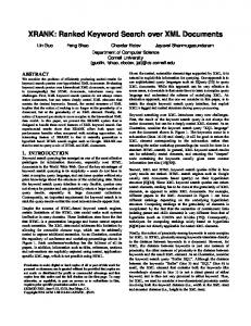
Figure 6: QPTs and PDTs of book and review from an XML view. We illustrate the QPT using the view shown in Figure 2. In order to evaluate this view query, we only need a small subset of the data, such as the isbn numbers of books and isbn numbers of reviews (which are required to perform a join). It is only when we want to materialize the view results do we need additional content such as the titles of books and content of reviews. The QPT is essentially a principled way of capturing this information. The QPT is a generalization of the Generalized Tree Patterns (GTP) [11], which was originally proposed in the context of evaluating complex XQuery queries. The GTP captures the structural parts of an XML document that are required for query processing. The QPT augments the GTP structure with two annotations, one that specifies which parts of the structure and associated data values are required during query evaluation, and the other that specifies which parts are required during result materialization. Figure 6(a) shows the QPTs for the book and review documents referenced in our running example. We first describe features present in the GTP. First, each QPT is associated with an XML document (determined by the view query). Second, as is usual in twigs, a double line edge denotes ancestor/descendant relationship and a single line edge denotes a parent/child relationship. Third, nodes are associated with tag names and (possibly) predicates. For instance, the year node in Figure 6(a) is associated with a predicate > 1995. Finally, edges in the QPT are either optional (represented by dotted lines) or mandatory (represented by solid lines). For example, in Figure 6(a), the edge between book and isbn is optional, because a book can be present in the view result even if it does not have an isbn number; the edge between review and isbn is mandatory, because a review is of no relevance to query execution unless it has an isbn number (otherwise, it does not join with any book and is hence irrelevant to the content of the view). The new features in the QPT are node annotations ’c’ and ’v’, where ’c’ indicates that the content of the node is propagated to the view output, and ’v’ indicates that the value of node is required to evaluate the view. In our example, the ’isbn’ node in both the book and review QPT is marked with a ’v’ since their values are required for performing a join operation; the ’title’ and ’content’ nodes are marked as ’c’ nodes since their content is propagated to the view

We now turn our attention to the PDT Generation Module (Figure 3), which is one of the main technical contributions in the paper. The PDT Generation Module efficiently generates a PDT for each QPT. Intuitively, the PDT only contains elements that correspond to nodes in the QPT and only contains element values that are required during query evaluation. For example, Figure 6(b) shows the PDT of the book document for its QPT shown in Figure 6(a). The PDT only contains elements corresponding to the nodes books, book, isbn, title, and year, and only the elements isbn and year have values. Using PDTs in our architecture offers two main advantages. First, the query evaluation is likely to be more efficient and scalable because the query evaluator processes pruned documents which are much smaller than the underlying data. Further, using PDTs allows us to use the regular (unmodified) query evaluator for keyword query processing. We note that the idea of creating small documents is similar to projecting XML documents (PROJ for short) proposed in [26]. There are, however, several key differences, both in semantics and in performance. First, while PROJ deals with isolated paths, we consider twigs with more complex semantics. As an example, consider the QPT for the book document in Figure 6(a). For the path books//book/isbn, PROJ would produce and materialize all elements corresponding to book (and its subelements corresponding to isbn). In contrast, we only produce book elements which have year subelements whose values are greater than 1995, which is enforced by the entire twig pattern. Second, instead of materializing every element as in PROJ, we selectively materialize a (small) portion of the elements. In our example, only the elements corresponding to isbn and year are materialized. Finally, the most important difference is that we construct the PDTs by solely using indices, while PROJ requires full scan of the underlying documents which is likely to be inefficient in our scenario. Our experimental results in Section 5 show that our PDT generation is more than an order of magnitude faster then PROJ. We now illustrate more details of PDTs before presenting our algorithms.

4.1 PDT Illustration & Definition The key idea of a PDT is that an element e in the document corresponding to a node n in the QPT is selected for inclusion only if it satisfies three types of constraints: (1) an ancestor constraint, which requires that an ancestor element of e that corresponds to the parent of n in the QPT should also be selected, (2) a descendant constraint, which requires that for each mandatory edge from n to a child of

1061

1:

n in the QPT, at least one child/descendant element of e corresponding to that child of n should also be selected, and (3) a predicate constraint, which requires that if e is a leaf node, it satisfies all predicates associated with n. Consequently, there is a mutual restriction between ancestor and descendant elements. In our example, only reviews with at least one isbn subelement are selected (due to the descendant constraint), and only those isbn and content elements that have a selected review are selected (due to the ancestor constraint). Note that this restriction is not “local”: a content element is not selected for a review if that review does not contain an isbn element. We now formally define notions of PDTs. We first define the notion of candidate elements that only captures descendant restrictions.

2: 3: 4: 5: 6: 7: 8: 9: 10: 11: 12: 13: 14: 15: 16: 17: 18: 19: 20: 21: 22: 23:

Definition 1 (candidate elements). Given a QPT Q, an XML document D, the set of candidate elements in D associated with a node n ∈ Q, denoted by CE(n, D), is defined recursively as follows. • n is a leaf node in Q: CE(n, D) = {v ∈ D | tag name of v is n.tag ∧ the value of v satisfies all predicates in n.preds }. • n is a non-leaf node in Q: CE(n, D) = {v ∈ D | tag name of v is n.tag ∧ for every edge e in Q, if e.parent is n and e.ann is ’m’ (mandatory), then ∃ec ∈ CE(e.child, D) such that (a) e.axis = ’/’ ⇒ v is the parent of ec, and (b) e.axis = ’//’ ⇒ v is an ancestor of ec } Definition 1 recursively captures the descendant constraints from bottom up. For example, in Figure 6(a), candidate elements corresponding to “review” must have a child element “isbn”. Now we define notions of PDT elements which capture both ancestor and descendant constraints. Definition 2 (PDT elements). Given a QPT Q, an XML document D, the set of PDT elements associated with a node n ∈ Q, denoted by PE(n, D), is defined recursively as follows. • n is the root node of Q: PE(n, D) = CE(n, D) • n is the non-root node in Q: PE(n, D) = {v ∈ D | v is in CE(n, D) ∧ for every edge e in Q, if e.child is n, then ∃vp ∈PE(e.parent, D) such that (a) e.axis = ’/’ ⇒ vp is the parent of v, and (b) e.axis = ’//’ ⇒ vp is an ancestor of v }

PrepareLists (QPT qpt, PathIndex pindex, InvertedIndex iindex, KeywordSet kwds): (PathLists, InvLists) pathLists ← ∅; invLists ← ∅ for Node n in qpt do p ← P athF romRoot(n); newList ← ∅ if n has no mandatory child edges then n.visited ← true if n has a ’v’ annotation then {Combining retrieval of IDs and values} newList ← (n, pindex.LookUpIDV alue(p)) else newList ← (n, pindex.LookUpID(p)) end if end if {Handle ’v’ nodes with mandatory child edges} if n.visited = f alse ∧ n has a ’v’ annotation then newList ← (n, pindex.LookUpIDV alue(p)) end if if newList 6= null then pathLists.add(newList) end for for all k in kwds do invLists ← invLists ∪ (k, sindex.lookup(k)) end for return (pathLists, invLists)

Figure 7: Retrieving IDs and values • N = ∪q∈Q PE(q, D), and nodes in N are associated with required values, tf values and byte lengths. • E = {(p, c) | p, c are in N ∧ p is an ancestor of c ∧ ∄q ∈ N s.t. p is an ancestor of q and q is an ancestor of c}

4.2 Proposed Algorithms We now propose our algorithm for efficiently generating PDTs. The generated PDTs satisfy all restrictions described above and contains selectively materialized element values. The main feature of our algorithm is that it issues a fixed number of index lookups in proportion to the size of the query, not the size of the underlying data, and only makes a single pass over the relevant path and inverted lists indices. At a high level, the development of the algorithm requires solving three technical problems. First, how do we minimize the number of index accesses? Second, how do we efficiently materialize required element values? Finally, how do we efficiently generate the PDTs using the information gathered from indices? We describe our solutions to these problems in turn in the next two sections.

4.2.1 Optimizing index probes and retrieving join values

Intuitively, the PDT elements associated with each QPT node are first the corresponding candidate elements and hence satisfy descendant constraints. Further, the PDT elements associated with the root QPT node are just its candidate elements, because the root node does not have any ancestor constraints; the PDT elements associated with a non-root QPT node have the additional restriction that they must have the parent/ancestors that are PDT elements associated the parent QPT node. For example, in Figure 6(a), each PDT element corresponding to “content” must have a parent element that is the PDT element with respect to “review”. Using the definition of PDT elements, we can now formally define a PDT. Definition 3 (PDT). Given a QPT Q, an XML document D, a set of keywords K, a PDT is a tree (N, E) where N is the set of nodes and E is set of edges, which are defined as follows.

To retrieve Dewey IDs and element values required in PDTs, our algorithm invokes a fixed number of probes on path indices. First, we issue index lookups for QPT nodes that do not have mandatory child edges; note that this includes all the leaf nodes. The elements corresponding to these nodes could be part of the PDT even if none of its descendants are present in the PDT according to the definition of mandatory edges [11]. Further, if a QPT node is associated with predicates, the index lookup will only return elements that satisfy the predicates. For instance, for the book QPT shown in Figure 6(a), we only need to perform three index lookups on path indices (shown in Figure 5) for three paths in QPT: books//book/isbn, books//book/year[.>1995], and books//book/title. Second, for nodes with ’v’ annotation, we issue separate lookups to retrieve their data values (which may be combined with the first round of lookups). The idea of retrieving values from path indices is inspired by a simple

1062

PrepareList():pathLists

1:

values

2: 3:

(books//book/isbn, (1.1.1: “111-11-1111”), (1.2.1: “121-23-1321”),... ) (books//book/title,1.1.4, 1.2.3, 1.9.3, …) (books//book/year, (1.2.6, 1.5.1: “1996”), (1.6.1:”1997"), …)

PrepareList():invLists

4: 5: 6: 7: 8: 9: 10:

tf values

(“xml”,(1.2.3:1),, (1.3.4:2), …) (“search”,(2.1.3:2), (2.5.1:1), …)

Figure 8: Results of PrepareLists() yet important observation that path indices already store element values in (Path, Value) pairs. Our algorithm conveniently propagates these values along with Dewey IDs. For example, consider the QPT of the book document in Figure 6(a) and the path indices in Figure 5. For the path books//book/isbn, we use its path to look up the B+-tree index over (Path, Value) pairs in the Path-Values table to identify all corresponding values and Dewey IDs (this can be done efficiently because Path is the prefix of the composite key, (Path, Value)); in Figure 5, we would retrieve the second and third rows from the Path-Values table. Note that IDs in individual rows are already sorted. We then merge the ID lists in both rows and generate a single list ordered by Dewey IDs, and also associate element values with the corresponding IDs. For example, the Dewey ID 1.1.1 will be associated with the value “111-111-1111”. Finally, our algorithm also returns the relevant inverted index indices to obtain scoring information. Figure 7 shows the high-level pseudo-code of our algorithm of retrieving Dewey IDs, element values and tf values. The algorithm takes a QPT, Path Index, query keywords, and Inverted Index as input, and first issues a lookup on path indices for each QPT node that has no mandatory child edges (lines 5- 13). It then identifies nodes that have a ’v’ annotation (lines 9 & 16), and for each path from the root to one of these nodes, the algorithm issues a query to obtain the values and IDs (by only specifying the path). Finally, the algorithm looks up inverted lists indices and retrieves the list of Dewey IDs containing the keywords along with tf values (lines 20-22). Figure 8 shows the output of PrepareList for the book QPT (Figure 6(a)). Note that the ID lists corresponding to books//book/isbn and books//book/year contain element values, and the ID lists retrieved from inverted lists indices contain tf values.

4.2.2 Efficiently generating PDTs In this section we propose a novel algorithm that makes a single “merge” pass over the lists produced by PrepareList and produces the PDT. The PDT satisfies the ancestor/descendant constraints (determined using Dewey IDs in pathLists) and contains selectively materialized element values (obtained from pathLists) and tf values w.r.t each query keyword (obtained from invLists). For our running example, our algorithm would produce the PDT shown in Figure 6(b) by merging the lists shown in Figure 8. The main challenges in designing such an algorithm are: (1) we must enforce complex ancestor and descendant constraints (described in Section 4.1) by scanning the lists of Dewey Ids only once, (2) ancestor/descendant axes may expand to full paths consisting of multiple IDs matching the same QPT nodes, which adds additional complication to the problem. The key idea of the algorithm is to process ids in Dewey order. By doing so, it can efficiently check descendant restric-

11: 12: 13: 14: 15: 16:

GeneratePDT (QPT qpt, PathIndex pindex, KeywordSet kwds, InvertedIndex iindex ): PDT pdt ← ∅ (pathLists, invLists) ← PrepareLists(qpt, pindex, iindex, kwds) for idlist ∈ pathLists do AddCTNode(CT.root, GetMinEntry(idlist), 0) end for while CT.hasMoreNodes() do for all n ∈ CT.MinIDPath do q ← n.QPTNode if pathLists(q).hasNextID() ∧ there do not exist ≥ 2 IDs in pathLists(q) and also in CT then AddCTNode(CT.root, pathLists(q).NextMin(), 0) end if end for CreatePDTNodes(CT.root, qpt, pdt) end while return pdt

Figure 9: Algorithm for generating PDTs tions because all descendants of an element will be clustered immediately after that element in pathLists. Figure 9 shows the high-level pseudo-code of our algorithm which works as follows. The algorithm takes in a QPT, path index and inverted index of the document, and begins by invoking PrepareList in order to collect the ordered lists of ids relevant to the view. It then initializes the Candidate Tree (described in more detail shortly) using the minimum ID in each list (lines 4-6). Next, the algorithm makes a single loop over the IDs in pathLists (lines 7-15), and creates PDT nodes using information stored in the CT. At each loop, the algorithm processes and removes the element corresponding to the minimum ID in the CT. Before processing and removing the element, it adds the next ID from the corresponding path list (lines 8-12) so that we maintain the invariant that there are at least one ID corresponding to each relevant QPT node for checking descendant constraints. Next the algorithm invokes the function CreatePDTNodes (line 14) and checks if the minimum element satisfies both ancestor and descendant constraints. If it does, we will create it in the result PDT. If it satisfies only descendant constraints, we store it in a temporary cache (PdtCache) so that we can check the ancestor constraints in subsequent loops. If it does not satisfies descendant constraints and does not have any children in the current CT, we discard it immediately. The intuition is that in this case, since the CT already contains at least one ID for each relevant QPT node (by the invariant above), and since IDs are retrieved from pathList in Dewey order, we can infer that the minimum element cannot have any unprocessed descendants in pathLists, hence it will not satisfy descendant constraints in all subsequent loops. The algorithm exits the loop and terminates after exhausting IDs in pathList and the result PDT contains all and only IDs that satisfy the PDT definition. We now describe the Candidate Tree and individual steps of the algorithm in more detail. Description of the Candidate Tree The Candidate Tree, or the CT, is a tree data structure. Each node cn in the CT stores sufficient information for efficiently checking ancestor and descendant constraints and has the following five components.

1063

• ID: the unique identifier of cn, which always corresponds to a prefix of a Dewey ID in pathLists. • QNode: the QPT node to which cn.ID corresponds. • ParentList (or PL): a list of cn’s ancestors whose QN-

1: 2: 3: 4: 5: 6: 7: 8: 9: 10: 11: 12: 13: 14: 15: 16: 17:

AddCTNode(CTNode parent, DeweyID id, int depth) newNode ← null if depth ≤ id.Length then curId←Prefix(id, depth); qNode←QPTNode(curId) if qNode = null then AddCTNode(parent,id,depth+1) else newNode ← parent.findChild(curId) if newNode = null then newNode ← parent.addChild(curId, qNode) Update the data value and tf values if required end if AddCTNode(newNode, id, depth+1) end if end if if newNode6=null ∧ ∀i, newNode.DM[i]=1 then ∀ n∈newNode.PL, n.DM[newNode.QPTNode]←1 end if

dummy root QNode: books ID: 1 DM:(book, 1) PL: null

book1 QNode: book ID: 1.1 DM:(year: 0) PL:

11: 12: 13: 14: 15: 16: 17: 18: 19: 20: 21:

books,1

book2 QNode: book ID: 1.2 DM: (year, 1) PL:

QNode: isbn ID: 1.1.1 DM :null PL:

QNode: title ID: 1.1.4 DM: null PL:

book,1.1

book,1.2

title,1.1.4

QNode: year ID: 1.2.6 DM: null PL:

year,1.2.6 New id

isbn,1.2.1

(b) Step 1: adding new ids to CT

(a) Initial CT root PdtCache: isbn,1.1.1

CreatePDTNodes (CTNode n, QPT qpt, PDT parentPdtCache) if ∀i, n.DM[i] = 1 ∧n.ID not in parentPdtCache then pdtNode = parentPdtCache.add(n) end if if n.HasChild() = true then CreatePDTNodes(n.MinIdChild, qpt, n.PdtCache) else {Handle pdt cache and then remove the node itself} for x in n.pdtCache do {Update parent list and then propagate x to parentPdtCache} if n ∈ x.PL then x.PL.remove(n) if ∃i, n.DM[i] = 0 ∧ x.PL = ∅ then n.pdtCache.remove(x) else x.PL.replace(n, n.PL) end if end if if x ∈ pdtCache then Propagate x to parentPdtCache end for n.RemoveFromCT() end if

isbn,1.1.1

root PdtCache: isbn,1.1.1 title,1.1.4

books,1

book,1.1

2: 3: 4: 5: 6: 7: 8: 9: 10:

root

isbn,1.1.1

Figure 10: Algorithm for adding new CT nodes 1:

DM: DescendantMap PL: ParentList

book,1.2

year,1.2.6 title,1.1.4 isbn,1.2.1

(c) Step 2: processing MinIDPath root PdtCache: isbn,1.2.1 title,1.2.3 year,1.2.6

PdtCache: book,1.2

books,1

book,1.2

book,1.1

isbn,1.2.1

book,1.2

title,1.2.3 year,1.2.6

(d) Step 3: before removing book,1.1 PdtCache: book,1.2 isbn,1.2.1 title,1.2.3 year,1.2.6

root books,1

...

...

(e) Before removing book,1.2

books,1

(f) Propagating nodes in pdt cache

Figure 12: Generating PDTs

Figure 11: Processing CT.MinIDPath ode’s are the parent node of cn.QNode. • DescendantMap (or DM):QNode→ bit: a mapping containing one entry for each mandatory child/descendant of cn.QNode. For a child QPT node c, DM[c] = 1 iff cn has a child/descendant node that is a candidate element with respect to c. • PdtCache: the cache storing cn’s descendants that satisfy descendant restrictions but whose ancestor restrictions are yet to be checked. We now illustrate these components using CT shown in Figure 12(a), which is created using IDs 1.1.1, 1.1.4, and 1.2.6, corresponding to paths in pathLists shown in Figure 8. First, every node has an ID and a QNode and CT nodes are ordered based on their IDs. For example, the ID of the “books” node is 1 which corresponds to a prefix of the ID 1.1.1, and the id 1.1.1 corresponds to the QPT node “isbn”. The PL of a CT node stores its ancestor nodes that correspond to the parent QPT node. For instance, book1.PL = {books}. Note that cn.PL may contain multiple nodes if cn.QNode is in an ancestor/descendant relations. For example, if “/books//book” expands to “/books/books/book”, then book.PL would include both “books”. Next, DM keeps track of whether a node satisfies descendant restrictions. For

instance, book1.DM[year] = 0 because it does not have the mandatory child element “year” while book2.DM[year] = 1 because it does. Consequently, a CT node satisfies the descendant restrictions (and therefore is a candidate element) when its DM is empty (corresponding to QPT nodes without mandatory child edges), or the values in its DM are all 1 (corresponding to QPT nodes with mandatory child edges). PdtCache will be illustrated in subsequent steps shortly. Note that for ease of exposition, our illustration focuses on creating the PDT hierarchy; the atomic values and tf values are not shown in the figure but bear in mind that they will be propagated along with Dewey IDs. Initializing the Candidate Tree As mentioned earlier, the algorithm begins by initializing the CT using minimum IDs in pathLists. Figure 10 shows the pseudo-code for adding a single Dewey ID and its prefixes to the CT. A prefix is added to the CT if it has a corresponding QPT node and is not already in the CT (lines 6-13). In addition, if a prefix is associated with a ’c’ annotation, the tf values are retrieved from the inverted lists (line 10). Figure 12(a), which we just described, shows the initial CT for our example, which is created by adding minimum IDs of paths in pathLists shown in Figure 8. Note that for ease of exposition, our algorithm assumes each Dewey ID corresponds to a single QPT node; however, when the QPT contains repeating tag names, one Dewey ID can correspond to multiple QPT nodes. We discuss how to handle this case in Section 4.2.2.1. Description of the main loop Next the algorithm enters the loop(lines 7-15 in Figure 9) which adds new Dewey IDs to the CT and creates PDT

1064

nodes using CT nodes. At each loop, the algorithm ensures the following invariant: the Dewey IDs that are processed and known to be PDT nodes are either in the CT or in the result PDT (hence we do not miss any potential PDT nodes); and the result PDT only contains IDs that satisfy the PDT definition. As mentioned earlier, at each loop we focus on the element corresponding to the minimum ID in the CT and its ancestors (denoted by MinIDPath in the algorithm). Specifically, we first retrieve next minimum IDs corresponding to QPT nodes in MinIDPath(Step 1). We then copy IDs in MinIDPath from top down to the result PDT or the PDT cache (Step 2). Finally, we remove those nodes in MinIDPath that do not have any children (Step 3). We now describe each step in more detail. Step 1: adding new IDs In this step, the algorithm adds the current minimum IDs in pathLists corresponding to the QPT nodes in CT.MinIDPath. In Figure 12(a), this path is “books//book/isbn” and Figure 12(b) shows the CT after its next minimum ID 1.2.1 is added (for reason of space, this figure and the rest only show the QPT node and ID). Step 2: creating PDT nodes In this step, the algorithm creates PDT nodes using CT nodes in CT.MinIDPath from top down (Figure 11, lines 2-4). We first check if the node satisfies the descendant constraints using values in its DM. In Figure 12(b), DM of the element “books” has value 1 in all entries, hence we will create its ID in the PDT cache passed to it(lines 2-4), which is the result PDT. The algorithm then recursively invokes CreatePDTNodes on the element book1 (line 6). Its DM has value 0 and hence it is not a PDT node yet. Next, we find its child element “isbn” has an empty DM and satisfies the descendant restrictions. Hence we create the node “isbn” in book1.PdtCache. Figure 12(c) illustrates this step. In general, the pdt cache of a CT node stores the ids of descendants that satisfy the descendant restrictions; ancestor restrictions are only checked when the CT node is removed (in Step 3). Step 3: removing CT nodes After the top down processing, the algorithm starts removing nodes from bottom up (Figure 11, line 7-20). For instance, in Figure 12(c), after we process and remove the node “title”, we will remove the node “book” because it does not have children and it does not satisfy descendant constraints. Figure 12(d) shows the CT at this point. Note that since we process nodes in id order, we can infer that the descendant constraints of this node will never be satisfied in the future. Another key issue we consider before removing a node is to handle nodes in its pdt cache. In our example, the pdt cache contains two nodes “isbn” and “title”. As mentioned earlier, they both satisfy descendant constraints. Hence we only need to check if they satisfy ancestor constraints, which is done by checking nodes in their parent lists. If those parent nodes are known to be non-PDT nodes, which is the case for “isbn” and “title”, then we can conclude the nodes in the cache will not satisfy ancestor restrictions, and can hence be removed (line 13). Otherwise the cache node still has other parents, which could be PDT nodes, and will thus be propagated to the pdt cache of the ancestor. Figure 6(e) and (f) illustrates this case in our running example, which occurs when we remove the node “book” with ID 1.2. Finally, at the last step of the algorithm when we remove the root node “books”, all IDs in its pdt cache will be propagated to the result PDT. In summary, we remove a node (and its ID) only when it is known to be a non-PDT node, which is either a CT node that does not satisfy descendant

constraints, or a node in a pdt cache that does not satisfy ancestor constraints. Further, we only create nodes satisfying descendant constraints in the pdt cache, and always check ancestor constraints before propagating them to ancestors in the CT. Therefore it is easy to verify that the invariant of the main loop holds.

4.2.2.1 Extensions and optimizations. As mentioned earlier, when the QPT has repeating tag names, a single Dewey ID can match multiple QPT nodes. For example, if the QPT path is “//a//a” and the corresponding full data path is “/a/a/a”, then the second “a” in the full path matches both nodes in the QPT path. To handle this case, we extend the structure of CT node to contain a set of QNodes, each of which is associated with their own InPdt, PL and DM. In general, different QPT nodes capture different ancestor/descendant constraints. Hence they must be treated separately. Further, there are two possible optimizations in the current algorithm. First, the algorithm always copies IDs that satisfy the descendant constraints in the pdt cache. This can be optimized by immediately creating the IDs in the result PDT if they also satisfy the ancestor restrictions. For this purpose, we add a boolean flag InPdt to the CT node, set InPdt to be true when the ID is created in the result PDT, and create the descendant ID in the PDT when one of its parents is in the PDT (InPdt = true). Second, to optimize the memory usage, we can output PDT nodes in document order (to external storage). We refer the reader to [35] for complete details and corresponding revisions to our algorithm.

4.2.2.2 Scoring & generating the results. As shown in Figure 3, once the PDTs are generated (e.g., the PDT of our running example is shown in Figure 6(b)), they are fed to a traditional evaluator to produce the temporary results, which are then sent to the Scoring & Materialization Module. Using just the pruned results with required tf values and byte lengths (encoded as XML attributes as shown in Figure 6(b)), this module first enforces conjunctive or disjunctive keyword semantics by checking the tf values, and then computes scores of the view results. Specifically, for a view result s, score(s) is computed as follows: first calculate tf (s, k) for a keyword k by aggregating values of tf (s′ , k) of all relevant base elements s′ ; then calculate the value idf (k) by counting the number of view results containing the keyword k; next use the formula in Section 2.2 to obtain the non-normalized scores, which are then normalized using aggregate byte lengths of the relevant base elements. The Scoring & Materialization Module then identifies the view results with top-k scores. Only after the final top-k results are identified are the contents of these results retrieved from the document storage system; consequently, only the content required for producing the results is retrieved.

4.3 Complexity and Correctness of Algorithms The runtime of GeneratePDT is O(N qdf + N qd2 + N d3 + N dkc) where N is the number of the IDs in pathLists, d is the depth of the document, q and f are the depth and fanout of the QPT, respectively, k is the number of keywords, and c is the average unit cost of retrieving tf values. Intuitively, the top-down and bottom-up processing dominate the overall cost. N qdf +N qd2 determines the cost of the topdown processing: there can be N d ID prefixes; every prefix can correspond to q QPT node; every QPT node can have d parent CT nodes and f mandatory child nodes. N d3 deter-

1065

Parameter Size of Data(×100M B) # keywords Selectivity of keywords # of joins Join selectivity Level of nestings # of results(K in top-K) Avg. Size of View Element

Values (default in bold) 1, 2, 3, 4, 5 1, 2, 3, 4, 5 Low(IEEE, Computing), Medium (Thomas, Control), High (Moore,Burnett) 0, 1, 2, 3, 4 1X, 0.5X, 0.2X, 0.1X 1, 2, 3, 4 1, 10, 20, 40 1X, 2X, 3X, 4X, 5X

We evaluated the performance of four alternative approaches: Baseline: materializing the view at the query time, and evaluating keyword search queries over views implemented using Quark. GTP: GTP with TermJoin for keyword searches and implemented using Timber [1]. Efficient: our proposed keyword query processing architecture (Section 3.1) developed using Quark, with all optimizations and extensions implemented(Section 4.2.2.1). Proj: techniques of projecting XML documents [26].

Table 1: Experimental parameters. mines the cost of bottom-up processing, since every prefix can be propagated d times and can have d nodes in its parent list. Finally, N dkc determines the cost of retrieving tf values from the inverted index. Note that this is a worst case bound which assumes multiple repeating tags in queries (q QPT nodes), and repeating tags in documents (d parent nodes). In most real-life data, these values are much smaller (e.g., DBLP4 , and SIGMOD Record5 , and INEX), as also seen in our experiments. We can prove the following correctness theorem (proofs are presented in [35]). If I is the function transforming Dewey IDs to node contents, PDTTF is the tf calculation function, and PDTByteLength is the byte length calculation function, len(e) is the byte length of a materialized element e, and using the notations of UD, Q, S defined in Section 2.1. Theorem 4.1 (Correctness). Given a set of keywords KW, an XQuery query Q and a database D ∈ UD, if PDTDB = {GeneratePDT(QPT, D.PathIndex, D.InvertedIndex, KW) | QPT ∈ GenerateQPT(Q) } , then • I(Q(PDTDB)) = Q(D)(The result sequences, after being transformed, are identical) • ∀e ∈ Q(PDTDB), e′ ∈ Q(D), I(e) = e′ ⇒ PDTByteLength(e) = len(e′ ) (The byte lengths of each element are identical) • ∀e ∈ Q(PDTDB), e′ ∈ Q(D), I(e) = e′ ⇒ (∀k ∈ KW, PDTTF(e,k) = tf(e′ ,k)) (The term frequencies of each keyword in each element is identical)

5.

EXPERIMENTS

In this section, we show the experimental results of evaluating our proposed techniques developed in the Quark opensource XML database system.

5.1 Experimental Setup In our experiments, we used the 500MB INEX dataset which consists of a large collection of publication records. The excerpt of the INEX DTD relevant to our experiments is shown below. journal (title, (sec1|article|sbt)*)> article (fno, doi?, fm, bdy)> fm (hdr?, (edinfo|au|kwd|fig)*)>

We created a view in which articles (article elements) are nested under their authors (au elements), and evaluated our system using this view. When running experiments, we generated the regular path and inverted lists indices implemented in Quark (∼1GB each). 4 5

http://dblp.uni-trier.de/xml/ http://acm.org/sigmod/record/xml/

We have implemented scoring in Efficient. Recall that our score computation (Section 4.2.2.2) produces exactly the same TF-IDF scores as if the view was materialized; hence, we do not evaluate the effectiveness of scoring using precision-recall experiments. Our experimental setup was characterized by parameters in Table 1. # of joins is the number of value joins in the view. Join selectivity characterizes how many articles are joined with a given author; the default value 1X corresponds to the entire 500MB data; we decrease the selectivity by replicating subsets of the data collection. Level of nestings specifies the number of nestings of FLOWR expressions in the view; for value 1, we remove the value join and only leave the selection predicate; for the default value 2, we associate publications under authors; for the deeper views, we create additional FLOWR expressions by nesting the view with one level shallower under the authors list. The rest of the parameters are self-explanatory. In the experiments, when we varied one parameter, we used the default values for the rest. The experiments were run on an Intel 3.4Ghz P4 processors running Windows XP with 2GB of main memory. The reported results are the average of five runs.

5.2 Performance Results 5.2.1 Varying size of data Figure 13 shows the performance results when varying the size of the data. As shown, it takes Efficient less than 5 seconds to evaluate a keyword query without materializing the view over the 500MB data. Second, the run time increases linearly with the size of the data (note that the y-axis is in log scale), because the index I/O cost and the overhead of query processing increases linearly. This indicates that Efficient is a scalable and efficient solution. In contrast, Baseline takes 59 seconds even for a 13MB data set, which is more than an order of magnitude slower than Efficient. Note the run time includes 58 seconds spent on materializing the view, and 1 second spent on the rest of query evaluation, including tokenizing the view and evaluating the keyword search query. Further, Figure 13 shows that Efficient performs ∼10 times faster than GTP. Note that Figure 13 only shows the time spent by GTP on structural joins and accessing the base data (for obtaining join values); it does not include the time for the remaining query evaluation since they were inefficient and did not scale well (the total running time for GTP, including the time to perform the value join, was more than 5 minutes on the 100MB data set). GTP is much slower mainly because it relies on (expensive) structural joins to generate the document hierarchy, and because it accesses base data to obtain join values. Finally, while Proj merely characterizes the cost of generating projected documents (the cost of query processing and post-processing are not included), its runtime is ∼15 times slower than Efficient. The main reason is that Proj scans

1066

64 32 16 8 4 2

Baseline GTP Proj Efficient

0.4 3

100

200

300

400

500

7 6 5 4 3 2 1 0

PDT

Evaluator

Post-processing

3

Size of Data(MB)

100

200

300

400

7 6 5 4 3 2 1 0

PDT

Evaluator

1

500

Size of Data(MB)

2

3 4 # of keywords

Figure 13: Varying size of Figure 14: Cost of Mod- Figure 15: keywords data ules base documents which leads to relatively poor scalability. For the rest of the experiments, we focus on Efficient since other alternatives performed significantly slower.

5.2.2 Evaluating Overhead of Individual Modules Figure 14 breaks down the run time of Efficient and shows the overhead of individual modules – PDT, Evaluator, and Post-processing. As shown, the cost of generating PDTs scales gracefully with the size of the data. Also, the overhead of post-processing, which includes scoring the results and materializing top-K elements, is negligible (which can be barely seen in the graphs). The most important observation is that the cost of the query evaluator dominates the entire cost when the size of the data increases.

5.2.3 Varying other parameters Varying # of keywords: Figure 15 shows the performance results when varying the number of keywords. The run time for Efficient increases slightly because it accesses more inverted lists to retrieve tf values. Varying # of joins: Figure 16 shows the performance results when varying the number of value joins in the view definition. As shown, the run time increases with the number of joins mainly because the cost of the query evaluation increases. The run time increases most significantly when the number of joins increases from 0 to 1 for two reasons. First, the case of 0 joins only requires generating a single PDT while the other requires two. More importantly, the cost of evaluating a selection predicate (in the case of 0 joins) is much cheaper than evaluating value joins. Other results: We also varied the size of the view element, the selectivity of keywords, the selectivity of joins, the level of nestings, and the number of results; the performance results (available in [35]) show that our approach is efficient and scalable with increased size of elements. Finally, the size of PDTs generated with respect to the entire data collection (500MB) is about 2MB, which indicates that our pruning techniques are effective.

6.

RELATED WORK

There has been a large body of work in the information retrieval community on scoring and indexing [21, 22, 32, 36]. However, they make the assumption that the documents being searched are materialized. In this paper, we build upon existing scoring and indexing techniques and extend them for virtual views. There has also been some recent interest on context-sensitive search and ranking [6], where the goal is to restrict the document collection being searched at run-time, and then evaluate and score results based on the restricted collection. In our terminology, this translates to ranked keyword search over simple selection views (e.g.,

7

Post-processing

Run time(seconds)

Run time (seconds)

128

Run time(seconds)

Run time(seconds)

256

5

6

PDT

Evaluator

Post-processing

5 4 3 2 1 0 0

1

2 # of Joins

3

4

Varying # Figure 16: Varying the number of joins

restricting searches to books with year > 1995). However, these techniques do not support more sophisticated views based on operations such as nested expressions and joins, which are crucial for defining even simple nested views (as in our running example). Supporting such complex operations requires a more careful analysis of the view query and introduces new challenges with respect to index usage and scoring, which are the main focus of this paper. In the database community, there has been a large body of work on answering queries over views (e.g., [7, 17, 34]), but these approaches do not support (ranked) keyword search queries. There has also been a lot of recent interest on ranked query operators, such as ranked join and aggregation operators for producing top-k results (e.g., [9, 31, 23]), where the focus is on evaluating complex queries over ranked inputs. Our work is complementary to this work in the sense that we focus on identifying the ranked inputs for a given query (using PDTs). There are, however, new challenges when applying these techniques in our context and we refer the reader to the conclusion for details. GTP [11] with TermJoin [1] were originally designed to integrate structure and keyword search queries. Since it is a general solution, it can also be applied to the problem of keyword search over views. However, there are two key aspects that make GTP with TermJoin less efficient in our context. First, GTP and TermJoin use relatively expensive structural joins to reconstruct the document hierarchy. Second, GTP requires accessing the base data to support value joins, which is again relatively inefficient. In contrast, our approach uses path indices to efficiently create the PDTs and retrieve join values, which leads to an order of magnitude improvement in performance (Section 5). Finally, our PDT generation technique is related to the technique for projecting XML documents [26]. The main difference is that we use indices to generate PDTs, which leads to a more than tenfold improvement in performance. We refer the reader to Section 4 for other technical differences between the two approaches. Our technique is also related to the projection operator in Timber [24] and lazy XSLT transformation of XML documents [33], which, like PROJ, also access the base data for projection.

7. CONCLUSION AND FUTURE WORK We have presented and evaluated a general technique for evaluating keyword search queries over views. Our experiments using the INEX data set show that the proposed technique is efficient over a wide range of parameters. There are several opportunities for future work. First, instead of using the regular query evaluator, we could use the techniques proposed for ranked query evaluation (e.g., [9, 16, 23]) to further improve the performance of our system.

1067

There are, however, new challenges that arise in our context because XQuery views may contain non-monotonic operators such as group-by. For example, when calculating the scores of our example view results, extra review elements may increase both the tf values and the document length, and hence the overall score may increase or decrease (nonmonotonic). Hence existing optimization techniques based on monotonicity are not directly applicable. Second, our proposed PDT algorithms may be applied to optimize regular queries because the algorithms efficiently generate the relevant pruned data, and only materialize the final results.

8.

ACKNOWLEGEMENTS

We thank Sihem Amer-Yahia at Yahoo! Research for her insightful comments on the draft of the paper. This work was partially funded by NSF CAREER Award IIS-0237644.

9.

REFERENCES

[1] S. Al-Khalifa, C. Yu, and H. V. Jagadish. Querying Structured Text in an XML Database. In SIGMOD, 2003. [2] S. Amer-Yahia et al. Structure and Content Scoring for XML. In VLDB, 2005. [3] A.Theobald and G. Weikum. The Index-Based XXL Search Engine for Querying XML Data with Relevance Rankings . 2002. [4] R. Baeza-Yates and B. Ribeiro-Neto. Modern Information Retrieval. ACM Press, 1999. [5] A. Bhaskar et al. Quark: An Efficient XQuery Full-Text Implementation. In SIGMOD, 2006. [6] C. Botev and J. Shanmugasundaram. Context-Sensitive Keyword Search and Ranking for XML. In WebDB, 2005. [7] M. J. Carey et al. XPERANTO: Middleware for Publishing Object-Relational Data as XML Documents. In The VLDB Journal, 2000. [8] C. Y. Chan, P. Felber, M. N. Garofalakis, and R. Rastogi. Efficient Filtering of XML Documents with XPath Expressions. VLDB Journal, 11(4), 2002. [9] S. Chaudhuri, L. Gravano, and A. Marian. Optimizing Top-k Selection Queries over Multimedia Repositories. IEEE Trans. Knowl. Data Eng., 16(8), 2004. [10] Z. Chen et al. Index Structures for Matching XML Twigs Using Relational Query Processors. Data Knowl. Eng., 60(2):283–302, 2007. [11] Z. Chen, H. V. Jagadish, L. V. S. Lakshmanan, and S. Paparizos. From Tree Patterns to Generalized Tree Patterns: On Efficient Evaluation of XQuery. In VLDB, 2003. [12] S. Cho. Indexing for XML Siblings. In WebDB, 2005. [13] V. Christophides, S. Cluet, and J. Simeon. On Wrapping Query Languages and Efficient XML Integration. In SIGMOD, 2000. [14] E. Curtmola, S. Amer-Yahia, P. Brown, and M. Fernandez. GalaTex: A Conformant Implementation of the XQuery Full-Text Language. In XIME-P, 2005. [15] Y. Diao, P. Fischer, M. Franklin, and R. To. YFilter: Efficient and Scalable Filtering of XML Documents. In ICDE, 2002. [16] R. Fagin. Combining Fuzzy Information from Multiple Systems. In PODS, 1996.

[17] G. Fahl and T. Risch. Query Processing Over Object Views of Relational Data. VLDB Journal, 6(4). [18] M. F. Fernandez, W. C. Tan, and D. Suciu. SilkRoute: trading between relations and XML. Computer Networks, 33(1-6), 2000. [19] N. Fuhr and K. Groβjohann. XIRQL: A Language for Information Retrieval in XML Documents. 2001. [20] L. Guo, F. Shao, C. Botev, and J. Shanmugasundaram. XRANK: Ranked Keyword Search over XML Documents. In SIGMOD, 2003. [21] V. Hristidis, L. Gravano, and Y. Papakonstantinou. Efficient IR-Style Keyword Search over Relational Databases. In VLDB, 2003. [22] V. Hristidis and Y. Papakonstantinou. Discover: Keyword Search in Relational Databases. In VLDB, 2002. [23] I. F. Ilyas et al. Rank-aware query optimization. In SIGMOD, 2004. [24] H. V. Jagadish et al. TIMBER: A Native XML Database. VLDB J., 11(4), 2002. [25] R. Kaushik, R. Krishnamurthy, J. F. Naughton, and R. Ramakrishnan. On the Integration of Structure Indexes and Inverted Lists. In ICDE, 2004. [26] A. Marian and J. Sim´eon. Projecting XML Documents. In VLDB, 2003. [27] Y. Mass et al. JuruXML – an XML retrieval system at INEX’02. In INEX, 2002. [28] S.-H. Myaeng, D.-H. Jang, M.-S. Kim, and Z.-C. Zhoo. A Flexible Model for Retrieval of SGML Documents. In SIGIR, 1998. [29] J. F. Naughton et al. The Niagara Internet Query System. IEEE Data Eng. Bull., 24(2), 2001. [30] P. O’Neil et al. ORDPATHs: Insert-Friendly XML Node Labels. In SIGMOD, 2004. [31] R.Fagin, A.Lotem, and M. Naor. Optimal Aggregation Algorithms for Middleware. In PODS, 2001. [32] G. Salton. Automatic Text Processing: The Transaction, Analysis and Retrieval of Information by Computer. Addison Wesley, 1989. [33] S. Schott and M. L. Noga. ”lazy xsl transformations”. In DocEng 2003, Grenoble, France, Nov 2003. ACM Press. [34] J. Shanmugasundaram et al. Querying XML Views of Relational Data. In VLDB, 2001. [35] F. Shao et al. Efficient Ranked Keyword Search over Virtual XML Views, Technical Report TR2007-2077, Cornell University. 2007. [36] I. H. Witten, A. Moffat, and T. C. Bell. Managing Gigabytes: Compressing and Indexing Documents and Images. Morgan Kaufmann Publishers, San Francisco, CA, 1999. [37] M. Yoshikawa and T. Amagasa. XRel: a path-based approach to storage and retrieval of XML documents using relational databases. ACM Trans. Inter. Tech., 1(1), 2001. [38] C. Zhang et al. On Supporting Containment Queries in Relational Database Management Systems. In SIGMOD, 2001. [39] J. Zobel and A. Moffat. Exploring the Similarlity Space. SIGIR Forum, 32(1), 2001.

1068