Hindawi Publishing Corporation Mathematical Problems in Engineering Volume 2016, Article ID 6392901, 14 pages http://dx.doi.org/10.1155/2016/6392901
Research Article Efficient Local Level Set Method without Reinitialization and Its Appliance to Topology Optimization Wenhui Zhang and Yaoting Zhang School of Civil Engineering and Mechanics, Huazhong University of Science and Technology, 1037 Luoyu Road, Wuhan 430074, China Correspondence should be addressed to Yaoting Zhang;
[email protected] Received 5 July 2015; Accepted 21 December 2015 Academic Editor: Manuel Pastor Copyright © 2016 W. Zhang and Y. Zhang. This is an open access article distributed under the Creative Commons Attribution License, which permits unrestricted use, distribution, and reproduction in any medium, provided the original work is properly cited. The local level set method (LLSM) is higher than the LSMs with global models in computational efficiency, because of the use of narrow-band model. The computational efficiency of the LLSM can be further increased by avoiding the reinitialization procedure by introducing a distance regularized equation (DRE). The numerical stability of the DRE can be ensured by a proposed conditionally stable difference scheme under reverse diffusion constraints. Nevertheless, the proposed method possesses no mechanism to nucleate new holes in the material domain for two-dimensional structures, so that a bidirectional evolutionary algorithm based on discrete level set functions is combined with the LLSM to replace the numerical process of hole nucleation. Numerical examples are given to show high computational efficiency and numerical stability of this algorithm for topology optimization.
1. Introduction Topology optimization is a numerical iterative procedure for making an optimal layout of a structure or the best distribution of material in the conceptual design stage [1]. The level set method (LSM) is a recently developed approach to topology optimization that uses a flexible implicit description of the material domain [2]. The central idea of the LSM is to employ an implicit boundary describing model to parameterize the geometric model, and the boundary of a structure is embedded in a high-dimensional level set function that is called its zero level set [3]. The level set-based method is able to not only fundamentally avoid checkerboards and mesh-dependence, but also maintain smooth boundaries and distinct material interfaces during the topological design process [4]. Hence, many level set-based methods [5] have been developed for topology optimization since the LSM was first introduced into structure optimization. With an implicit local level set model, the computational efficiency of the local level set method (LLSM) [6] is much higher than that of the global level set methods, especially for shape optimization. However, the main shortcoming of the conventional LSM is that it possesses no mechanism
to nucleate new holes in the material domain for twodimensional structures, resulting in the final design heavily dependent on the initial guess [4]. A mechanism named the bubble-method [7] was first proposed to create new holes inside the structures in topology and shape optimization. This idea has been further developed into the mathematical concept of topological derivatives [8]. In the shapesensitivity-based level set approaches, topological derivatives are incorporated to indicate the best place for introducing a new hole in a separate step of the optimization process [9] or as an additional term in the Hamilton-Jacobi equation [10]. The globally supported radial basis function (RBF) [11] and compactly supported RBF (CSRBF) [12] are typically used to discretize the original time-dependent initial value problem into an interpolation problem. The CSRBF brings about the strictly positive definiteness and sparseness properties of matrices under certain conditions. Hence the CSRBF has generalized the practical applications of RBFs to a larger set of scattered data [12]. In the conventional LSM [3], a reinitialization procedure usually needs to reshape the level set function (LSF) to a signed distance function (SDF) periodically. However, the zero level set may drift away from its initial position by
2
Mathematical Problems in Engineering
iteratively solving a classical reinitialization equation [13]. To suppress this drift, an interface preserving level set redistancing algorithm is proposed by Sussman and Fatemi [14]. Nevertheless, it has been proved that the SDF is not a feasible solution to the H-J equation [15]. In practice, it not only raises serious problems as when and how it should be performed, but also affects numerical accuracy in an undesirable way and thus should be avoided as much as possible [16]. The need for reinitialization was originally eliminated by introducing a penalty term [17] into a variational level set approach [18]. The undesirable boundary effect of the penalty term can be eliminated by taking a distance regularized equation (DRE) instead of this term. Hence, a so-called distance regularized level set evolution (DRLSE) [16] is realized based on the variational approach. As an unnecessary diffusion effect of the DRLSE was found in some locations where the surface is too flat, the DRE was recently modified with a new and balanced formulation to eliminate this effect [19]. Although parts of the diffusion rates in the DRE are negative, the numerical stability can still be maintained by incorporating reverse diffusion constraints in the difference schemes of the DRE, as can the reverse diffusion equations with all negative diffusion rates [20]. The aim of this work is to solve the aforementioned numerical issues that still exist in the LLSM for topology optimization of two-dimensional structures. A bidirectional evolutionary algorithm based on the discrete level set functions (DLSFs) is proposed to find a stable topological solution first and then combined with the LLSM to further evolve the local details of the topology and shape of the structure. Transforming the DLSFs into the local level set function of the LLSM is achieved by iteratively solving the DRE. After that, the DRE is incorporated into the LLSM to avoid the reinitialization procedure. A difference scheme under reverse diffusion constraints is formulated for the DRE to improve its numerical stability. Typical examples are given to show the effectiveness of the proposed algorithm in terms of convergence, computational efficiency, and numerical stability.
2. Optimization Algorithm 2.1. Local Level Set Method Using Narrow-Band Model. In the local level set method (LLSM) [6], the local level set equation is defined as 𝜕𝜙 + 𝐶 (𝜙) 𝑉𝑛 ∇𝜙 = 0, 𝜕𝑡
(1)
where 𝜙(𝑥, 𝑡) is defined as the local level set function (LLSF) and 𝑉𝑛 is the normal velocity in normal direction 𝑛 = ∇𝜙/|∇𝜙|; the truncation function 𝐶(𝜙) is 1 { { { { 2 { 𝐶 (𝜙) = { (𝜙 − 𝛾) (2 𝜙 + 𝛾 − 3Δ) 3 { { (𝛾 − Δ) { { {0
if 𝜙 ≤ Δ if Δ < 𝜙 ≤ 𝛾 (2) if 𝜙 > 𝛾,
with 𝑇0 = {𝑥 : 𝜙(𝑥) < 𝛾} being a narrow band with the half-band width 𝛾. The narrow-band model and the corresponding LLSF are described as shown in Figure 1. It can be seen from Figure 1 that only the LLSF within the narrow-band 𝑇0 needs to be updated during each iteration. Hence, the LLSM is higher in computational efficiency than the LSMs based on global level set models. 2.2. Bidirectional Evolutionary Algorithm with Discrete Level Set Functions. A two-dimensional structural model is built in the work region 𝐷 ⊂ 𝑅2 . And the set 𝑆 = 𝑆1 ∪ 𝑆2 ∪ 𝑆3 represents the finite elements in the domain 𝐷. It can be divided into three parts, 𝑆1 that consists of the solid elements with a full-material density; 𝑆2 that covers the elements with intermediate material densities; 𝑆3 that involves the void elements with a weak-material density. Accordingly, the nodal sets corresponding to the elemental sets 𝑆1 , 𝑆2 , and 𝑆3 are defined as 𝑆1𝑛 , 𝑆2𝑛 , and 𝑆3𝑛 , respectively. If it is assumed that 𝑆2𝑛 ⊂ 𝑆3𝑛 , 𝑆1𝑛 ∪ 𝑆3𝑛 consist of all the nodes within the region 𝐷, then a discrete level set function (DLSF) for node 𝑗 can be defined as {−𝑐0 𝜙𝑗 = { 𝑐 {0
𝑗 ∈ 𝑆1𝑛 𝑗 ∈ 𝑆3𝑛 ,
(3)
where 𝑐0 is a predefined constant set as 1 in this study. The values of elemental densities can be derived from the DLSFs. If the 𝑖th element belongs to 𝑆1 , that is, 𝑖 ∈ 𝑆1 , then the element density 𝜌𝑖 = 1; if 𝑖 ∈ 𝑆3 , then 𝜌𝑖 = 𝜌min , where 𝜌min is a small value 0.001; if 𝑖 ∈ 𝑆2 , then 𝜌𝑖 ∈ (𝜌min , 1), where 𝜌𝑖 is calculated in terms of the interpolation criterion given in the code manual [21]. In the structural model, the rectangular element is split into four triangles first, and the value of the DLSF at the common point of the triangles is then given by the average of the values of the four points. After that, each triangle is examined separately in the same logic. Finally, the elemental density is found to be the average of the contributions of the triangles. The structural stiffness design has been widely investigated in numerous literatures for topological sensitivity analysis. The standard notion [1] of minimum compliance design problems under a global volume constraint can be mathematically defined as follows: 1 minimize 𝐽 (Ω) = 𝑢𝑇 𝐾𝑢, 𝜙 2 𝑁
Subject to
∑𝑉𝑖 𝜌𝑖 (𝜙) = 𝑉∗ ,
(4)
𝑖=1
𝜌𝑖 ∈ [𝜌min , 1] , where 𝐽 is known as the mean compliance, the open set Ω represents all admissible shapes in the design region 𝐷, 𝑢(𝜙) is the nodal displacement vector, and 𝐾 denotes the global stiffness matrix; 𝑉𝑖 is the volume of an individual element, 𝑉∗ is the prescribed total volume, and 𝑁 is the number of elements.
Mathematical Problems in Engineering
3
2𝛾 Ω
D\Ω
Edge of narrow band Zero level set
Ω D\Ω
𝜙 c0
0
𝛾
x
−c0
Figure 1: Narrow-band model and local level set function in LLSM.
Similar to the bubble-method [7] and the level set-based optimization methods [4, 10], topological derivatives are taken as topological sensitivities in this study. The topological derivative for node 𝑗 is given by [9] 𝛼𝑗𝑛 = 𝐷𝑇 𝐽 (𝜙𝑗 ) =
𝜋 (𝜆 + 2𝜇) {4𝜇𝐸𝑗 𝜀 (𝑢) : 𝜀 (𝑢) 4𝜇 (𝜆 + 𝜇)
(5)
+ (𝜆 − 𝜇) tr (𝐸𝑗 𝜀 (𝑢)) tr (𝜀 (𝑢))} , where 𝐸𝑗 denotes the material elasticity tensor for node 𝑗, 𝜀 is the strain tensor, and the lame constants 𝜆 = 𝐸0 ]/(1 − ]2 ), 𝜇 = 𝐸0 /2(1 + ]) with the Poisson ratio ] and Young’s modulus of solid materials 𝐸0 . tr(𝐴) denotes the trace of a matrix 𝐴. Based on an interpolation function proposed by Shepard [22], a filter scheme of mesh independence is proposed to avoid the checkerboard patterns and mesh dependencies. A circular domain Ω𝑤 is first defined as the influence region centered round point x with cut-off radius 𝑟𝑤 , and 𝑁Ω denotes the number of points located inside the influence domain. The sensitivity filtering using the Shepard method with scattered points is then defined by 𝑁Ω
̃ 𝑛 (x) = ∑𝑊𝑖 (x) ⋅ 𝛼𝑛 (x) , 𝛼
where 𝑊𝑖 (x) is the Shepard interpolation with the basis function 𝐷𝑖 (x) = 1/√(𝑑𝑖 (x))2 + 𝑐2 , in which 𝑑𝑖 (x) = ‖x − 𝑥𝑖 ‖ denotes the radial distance from point 𝑥 to 𝑥𝑖 , and if 𝑑𝑖 (x) ≥ 𝑟𝑤 , then 𝐷𝑖 (x) is set to zero. 𝑐 is a positive constant and chosen as a onefold mesh size in terms of numerical experiences. Over the last two decades, many topology description models have been developed for topology optimization of structures, which can roughly be classified into two categories, the material distribution model and the boundary description model [23]. Based on the material distribution model, the ESO (Evolutionary Structural Optimization) method has won a great deal of popularity in recent years [24]. The bidirectional ESO (BESO) method [25], as an extension of the ESO method, allows efficient material to be added to the structure while the inefficient one is removed simultaneously. So a bidirectional evolutionary algorithm is developed by integrating both the DLSFs and topological derivatives into the optimization criteria of the BESO method [25]. Note that the design variables and topological sensitivities in the BESO method are based on the elemental pseudo densities while those in the proposed algorithm are based on the discrete level set functions. It is assumed that the volume in the 𝑘th iteration 𝑉𝑘 is known, and 𝑘 ≥ 0. The target volume 𝑉𝑘+1 in the next iteration is then updated by
𝑖=1
𝑊𝑖 (x) =
𝐷𝑖 (x)
∑𝑁 𝑗=1
(6)
𝐷𝑗 (x) (𝑖 = 1, . . . , 𝑁) ,
𝑉𝑘+1
∗ ∗ {min (𝑉𝑘 (1 + ER) , 𝑉 ) if 𝑉𝑘 ≤ 𝑉 ={ max (𝑉𝑘 (1 − ER) , 𝑉∗ ) if 𝑉𝑘 > 𝑉∗ {
(7)
with the evolutionary volume ratio ER and the volume limit 𝑉∗ defined in (4).
4
Mathematical Problems in Engineering
A parameter AR𝑛 is defined as the adding number of nodes in the set 𝑆1𝑛 divided by the total numbers of 𝑛 𝑛 , where ARmax is a predefined nodes and AR𝑛 ≤ ARmax positive constant. The definition of AR𝑛 is different from that of AR in the original BESO method, since the former parameter corresponds to nodal sensitivity while the latter one corresponds to elemental sensitivity. It is assumed that the DLSF 𝜙𝑗𝑘 of node 𝑗 is known in
the 𝑘th iteration. Then the DLSF 𝜙𝑗𝑘+1 in the next iteration is updated by
𝜙𝑗𝑘+1
{−𝑐0 ={ {𝑐0
add 𝛼𝑗𝑛 ≥ 𝛼th , 𝜙𝑗𝑘 = 𝑐0 del 𝛼𝑗𝑛 ≥ 𝛼th , 𝜙𝑗𝑘 = −𝑐0 ,
(8)
del add where the threshold sensitivity numbers 𝛼th and 𝛼th are determined as the number of nodes decreased from the set 𝑆1𝑛 and that increased from the set 𝑆3𝑛 , respectively. These thresholds are similar to those based on elemental sensitivities given in the original BESO method. Full details of determining these thresholds are described in [25]. Finally, a stable topological solution is obtained when the following convergence criterion is satisfied:
𝑘−5 ∑𝑘−9 𝐽 (Ω) − ∑𝑘𝑘−4 𝐽 (Ω) ≤ 𝜏, ∑𝑘𝑘−4 𝐽 (Ω)
(9)
where 𝜏 is an allowable convergence error with typical values ranging from 0.001 to 0.01. The majority of logical steps of the bidirectional evolutionary algorithm are presented in Figure 2. 2.3. Distance Regularized Equation (DRE) and Its Improvement. In the distance regularized level set evolution (DRLSE) [16], the DRE can retain the signed distance feature |∇𝜙| = 1 at least within the narrow-band region near boundaries without reinitialization, whose formula is expressed in the standard form of the diffusion equation as 𝜕𝜙 = 𝜇 div (𝛼1 (𝜙) ∇𝜙) , 𝜕𝑡
(10)
with the diffusion rate 𝛼1 (𝜙) = 𝜇𝑑𝑝1 (|∇𝜙|), where the diffusion function is set to 𝑑𝑝1 (𝑠) = 𝑝1 (𝑠)/𝑠 with 𝑠 = |∇𝜙|. In the original DRLSE, the energy density 𝑝1 (𝑠) was defined as (1 − cos (2𝜋𝑠)) { { { (2𝜋)2 { 𝑝1 (𝑠) = { { 2 { { (𝑠 − 1) { 2
if 𝑠 ≤ 1 (11) if 𝑠 > 1,
which is a double-well potential function because there are two minimum points of 𝑝1 (𝑠) at 𝑠 = 1 and 𝑠 = 0. So the diffusion function 𝑑𝑝1 (𝑠) is given by sin (2𝜋𝑠) { { { { 2𝜋𝑠 𝑑𝑝1 (𝑠) = { { { {1 − 1 { 𝑠
if 𝑠 ≤ 1 (12) if 𝑠 > 1.
It is easy to verify the boundedness of the diffusion rate 𝛼1 (𝜙) = 𝜇𝑑𝑝1 (|∇𝜙|) and |𝛼1 (𝜙)| ≤ 𝜇. It can be seen from (12) that, for |∇𝜙| > 1, 𝑑𝑝1 (|∇𝜙|) is positive, and |∇𝜙| will decrease and approach 1; for 0.5 < |∇𝜙| ≤ 1, 𝑑𝑝1 (|∇𝜙|) is negative, and |∇𝜙| will increase and approach 1; for |∇𝜙| ≤ 0.5, 𝑑𝑝1 (|∇𝜙|) is positive, and |∇𝜙| will decrease and approach 0. If |∇𝜙0 | ≤ 0.5 is satisfied for all the initial values 𝜙0 , the diffusion effect of (10) will make |∇𝜙| approach 0. So it loses the ability to regularize |∇𝜙| to 1. An improved diffusion rate 𝛼2 (𝜙) with a diffusion function like the following is proposed in [19]: 2 { { { { 𝜋 arctan (( { ∇𝜙 − 1) /𝜎) 𝑑𝑝2 (∇𝜙) = { { { 2 { { 𝜋 arctan ((∇𝜙 − 1) /𝜎) {
𝜙 ≤ 𝜀 𝜙 > 𝜀,
(13)
where 𝜎 is a positive constant and is chosen as fourfold mesh sizes in terms of numerical experiences. 𝑇1 = {𝑥 : 𝜙(𝑥) < 𝜀} is a narrow band with a half-band width 𝜀. The diffusion effect can be divided into two parts: the forward diffusion for |∇𝜙| ≥ 1 and the backward diffusion for |∇𝜙| < 1. It will make |∇𝜙| approach one within 𝑇1 but zero outside 𝑇1 . However, the two parts are balanced within 𝑇1 but unbalanced outside 𝑇1 so that multiple iterations are required to retain a flatter level set surface outside 𝑇1 . In this paper, the diffusion function 𝑑𝑝2 (|∇𝜙|) is further localized by introducing the half-band width 𝛾 of the narrow-band 𝑇0 in LLSM, thereby resulting in an improved diffusion rate 𝛼3 (𝜙) using the diffusion function 2 { 𝜋 arctan (( 𝑑𝑝3 (∇𝜙) = { ∇𝜙 − 1) /𝜎) {0
𝜙 < 𝛾 𝜙 ≥ 𝛾.
(14)
With the diffusion rate 𝛼3 (𝜙), the two parts are balanced within 𝑇0 without influencing the level set surface outside 𝑇0 . 2.4. A Conditionally Stable Difference Scheme for DRE. It is noted that the common difference schemes for the DRE with parts of the negative diffusion rates are incapable of remaining stable during an iterative process, according to the stability definition of the difference equation. In our numerical experiments, |𝜙| is apt to gradually become divergent along with the process of iterations. To enhance the numerical
Mathematical Problems in Engineering
5
Start
Define the maximum design domain, initial design, loads, and supports
Define the elemental set S and the initial DLSFs 𝜙0j
Determine the target volume for the next iteration Vk+1
Carry out the finite element analysis; calculate the topological derivative of each node
Update the topological derivatives by sensitivity filtering using Shepard interpolation function Increase the iteration number k = k + 1 Update the DLSFs 𝜙k+1 according to the j optimization criterion of BESO method No
Is the convergence criterion satisfied?
Yes Stop iteration and obtain a stable topological solution
Figure 2: Flow chart depicting logical steps of the bidirectional evolutionary algorithm.
stability of the DRE, a difference scheme similar to that of the mean curvature given in [18] is developed and described as 𝑘+1 𝑘 − 𝜙𝑖,𝑗 𝜙𝑖,𝑗
Δ𝑡
=
𝛼 (𝜙𝑘 )𝑖+1/2,𝑗 𝛿+𝑥 𝜙𝑖,𝑗 − 𝛼 (𝜙𝑘 )𝑖−1/2,𝑗 𝛿−𝑥 𝜙𝑖,𝑗
+
Δ𝑥 𝑦 𝑦 𝛼 (𝜙𝑘 )𝑖,𝑗+1/2 𝛿+ 𝜙𝑖,𝑗 − 𝛼 (𝜙𝑘 )𝑖,𝑗−1/2 𝛿− 𝜙𝑖,𝑗 Δ𝑦
, (15)
6
Mathematical Problems in Engineering
where
Then the four flow functions are defined as 𝛿+𝑥 𝜙𝑖,𝑗 = 𝛿𝑐𝑥 𝜙𝑖,𝑗 = 𝛿−𝑥 𝜙𝑖,𝑗 = 𝛿+𝑦 𝜙𝑖,𝑗
=
𝛿𝑐𝑦 𝜙𝑖,𝑗 = 𝛿−𝑦 𝜙𝑖,𝑗 =
𝑘 (𝜙𝑖+1,𝑗
−
𝑘 𝜙𝑖,𝑗 )
Δ𝑥
𝑘 𝑘 (𝜙𝑖+1,𝑗 − 𝜙𝑖−1,𝑗 )
(2Δ𝑥) 𝑘 𝑘 (𝜙𝑖,𝑗 − 𝜙𝑖−1,𝑗 )
Δ𝑥 𝑘 (𝜙𝑖,𝑗+1
𝑘 − 𝜙𝑖,𝑗 )
Δ𝑦
,
𝑦
𝑘 𝑘 − 𝜙𝑖,𝑗 ) 𝛼𝑖,𝑗+1/2 , 𝐹𝑖,𝑗 = (𝜙𝑖,𝑗+1 𝑦
, ,
,
𝑦
2
𝑥
2
(17)
Δ𝑡 ) Δ𝑥
Δ𝑡 ) Δ𝑦
(18)
𝑘 𝑘 𝑘 𝑘 − 𝜙𝑖,𝑗 ) 𝛼𝑖,𝑗+1/2 + (𝜙𝑖,𝑗−1 − 𝜙𝑖,𝑗 ) 𝛼𝑖,𝑗−1/2 ] , ⋅ [(𝜙𝑖,𝑗+1
(1/Δ𝑥)𝛼(𝜙𝑘 )𝑖+1/2,𝑗 and 𝛼𝑖,𝑗±1/2
𝑦
𝑥 𝑥 , 𝐹𝑖−1,𝑗 , 𝐹𝑖,𝑗 , 𝐹𝑖,𝑗−1 ≤ 𝐹high . 𝐹low ≤ 𝐹𝑖,𝑗
(21)
If Δ𝑡/Δ𝑥 ≤ 1/4, first substituting (20) into inequalities (21) and then substituting the result into (18), one can obtain a solution using the inequalities
𝑘 𝑘 𝑘 𝑘 ⋅ [(𝜙𝑖+1,𝑗 − 𝜙𝑖,𝑗 ) 𝛼𝑖+1/2,𝑗 + (𝜙𝑖−1,𝑗 − 𝜙𝑖,𝑗 ) 𝛼𝑖−1/2,𝑗 ] ,
= with 𝛼𝑖±1/2,𝑗 𝑘 (1/Δ𝑦)𝛼(𝜙 )𝑖,𝑗±1/2 .
(20)
It can be seen that the four diffusion rates in (15) satisfy the boundedness |𝛼(𝜙𝑘 )| ≤ 𝜇. If 𝜇 ≤ Δ𝑥, the reverse diffusion constraints can be defined by 𝑦
It has been verified by our numerical experiments that the evolution of level set can remain bounded stability even after a large number of iterations for solving (15). However, the maximum of |𝜙| often exceeds the initial value 𝑐0 defined by (1), which leads to the level set surface unsmoothed near the edges of the narrow-band 𝑇0 , thereby reducing the computational accuracy of (15). Furthermore, multiple iterations are required to find a suitable Courant-FriedrichsLewy (CFL) condition to ensure the stability of (15). The issues related to the numerical instability of the DRE can be resolved by imposing reverse diffusion constraints on the difference scheme (see (15)), since it has been proved that the constraints can ensure the numerical stability of the diffusion equations with all negative diffusion rates [20]. First, (15) can be subdivided along the direction of 𝑥 and 𝑦 into
𝑘+1 𝑘+1/2 𝜙𝑖,𝑗 − 𝜙𝑖,𝑗 =(
𝑘 − 𝜙𝑖,𝑗 ,
𝑝,𝑞=−1,0,1
(𝛿𝑐 𝜙𝑖,𝑗 + 𝛿𝑐 𝜙𝑖±1,𝑗 ) 2 𝑦 ]. ∇𝜙𝑖,𝑗±1/2 = √ (𝛿± 𝜙𝑖,𝑗 ) + [ 2
𝑘+1/2 𝑘 − 𝜙𝑖,𝑗 =( 𝜙𝑖,𝑗
min 𝜙𝑘 𝑝,𝑞=−1,0,1 𝑖+𝑝,𝑗+𝑞
𝑘 𝑘 − 𝜙𝑖,𝑗 . 𝐹high = max 𝜙𝑖+𝑝,𝑗+𝑞
(𝛿𝑐 𝜙𝑖,𝑗 + 𝛿𝑐 𝜙𝑖±1,𝑗 ) 2 ], ∇𝜙𝑖±1/2,𝑗 = √ (𝛿±𝑥 𝜙𝑖,𝑗 ) + [ 2 𝑥
𝑥 𝑘 𝑘 denotes the change from 𝜙𝑖,𝑗 to 𝜙𝑖+1,𝑗 in one time where 𝐹𝑖,𝑗 𝑦 𝑥 step Δ𝑡 and in the 𝑥 direction, and the definitions of 𝐹𝑖,𝑗 , 𝐹𝑖,𝑗 , 𝑦 𝑥 and 𝐹𝑖,𝑗−1 are similar to that of 𝐹𝑖,𝑗 . The lowest and highest limit values of these flow functions are defined as
𝐹low =
and 𝛼(𝜙) fl 𝛼3 (𝜙), in which the difference schemes of |∇𝜙|𝑖±1/2,𝑗 , |∇𝜙|𝑖,𝑗±1/2 are given by 𝑦
(19)
𝑘 𝑘 𝐹𝑖−1,𝑗 = (𝜙𝑖,𝑗−1 − 𝜙𝑖,𝑗 ) 𝛼𝑖,𝑗−1/2 ,
(16)
(2Δ𝑦) Δ𝑦
𝑥 𝑘 𝑘 = (𝜙𝑖−1,𝑗 − 𝜙𝑖,𝑗 ) 𝛼𝑖−1/2,𝑗 , 𝐹𝑖−1,𝑗
,
𝑘 𝑘 (𝜙𝑖,𝑗+1 − 𝜙𝑖,𝑗−1 )
𝑘 𝑘 (𝜙𝑖,𝑗 − 𝜙𝑖,𝑗−1 )
𝑥 𝑘 𝑘 = (𝜙𝑖+1,𝑗 − 𝜙𝑖,𝑗 ) 𝛼𝑖+1/2,𝑗 , 𝐹𝑖,𝑗
,
=
min 𝜙𝑘 𝑝,𝑞=−1,0,1 𝑖+𝑝,𝑗+𝑞
𝑘+1 𝑘 ≤ 𝜙𝑖,𝑗 ≤ max 𝜙𝑖+𝑝,𝑗+𝑞 . 𝑝,𝑞=−1,0,1
(22)
𝑘 It can be seen that the absolute values of 𝜙𝑖+𝑝,𝑗+𝑞 for 𝑝, 𝑞 = −1, 0, 1 are lower than their initial value 𝑐0 . That means that all the absolute values |𝜙| ≤ 𝑐0 if the CFL conditions are satisfied:
𝜇Δ𝑡 1 ≤ , Δ𝑥2 4 𝜇Δ𝑡 1 ≤ . Δ𝑦2 4
(23)
2.5. Flow Chart for Difference Schemes to LLSM with DRE. The procedure for the LLSM with the DRE consists of two main parts, transforming the models of discrete level set functions into the local level set function and solving the difference schemes of the LLSE associated with the DRE. The final DLSFs corresponding to the stable topological solution can be transformed into the LLSF within the initial narrowband 𝑇0 by iteratively solving the DRE under reverse diffusion constraints. The LLSE can be solved by difference schemes using the third-order Runge-Kutta (R-K) scheme for temporal discretization and the fifth-order weighted essentially nonoscillatory (WENO) scheme for spatial discretization. The reader is referred to [26] for more numerical details. The logical steps of the two parts can be described by a flow chart given in Figure 3.
Mathematical Problems in Engineering
7
Transforming DLSFs into LLSF The DLSF 𝜙nj of stable topological solution
Define an initial diffusion rate 𝛼0 (𝜙) with dp0 (|∇𝜙|) = 2/𝜋 arctan((|∇𝜙| − 1)/𝜎)
Iteratively solve the DRE with 𝛼0 (𝜙) 100 times and gain the half-band width 𝛾
Restart from the DLSFs according to the stable topological solution 𝜙nj
Transform the DLSFs into the LLSF 𝜙 by iteratively solving the DRE with 𝛼3 (𝜙) under reverse diffusion constraints
Solve the LLSE while iteratively solving the DRE with 𝛼3 (𝜙) under reverse diffusion constraints until the LLSF 𝜙 is sufficiently smooth within T0
Increase the iteration number k = k + 1
Is the convergence critertion satisfied
No
Yes
End
Figure 3: Flow chart depicting logical steps of the LLSM.
8
Mathematical Problems in Engineering
2.6. Shape Derivatives and Normal Extension Velocities. With the classical level set model [4], the minimum compliance design problem given in (4) can be converted to an unconstrained problem with the Lagrangian method: Minimize 𝐿 (𝑢, 𝜙) 𝜙
∗
(24)
= 𝐽 (𝑢, 𝜙) + 𝜆 + (∫ 𝐻 (𝜙) 𝑑Ω − 𝑉 ) , 𝐷
where the Lagrangian function 𝐿(𝑢, 𝜙) is the objective functional. 𝜆 + is the Lagrangian multiplier of the volume constraint. 𝐻(𝜙) is the Heaviside function. The mean compliance 𝐽(𝑢, 𝜙) is reformulated as 𝐽 (𝑢, 𝜙) =
1 ∫ 𝐸𝜀 (𝑢) : 𝜀 (𝑢) 𝐻 (𝜙) 𝑑Ω. 2 𝐷
(25)
For a number of level set-based approaches [4, 9, 11, 12], the steepest descent method is used to ensure the decrease of the objective function by directly setting the normal velocity field 𝑉𝑛 as the negative shape derivative of 𝐿(𝑢, 𝜙). For the particular case of a 2-D model of a linear elastic structure, the boundary traction is fixed and remains unchanged, the displacement constraint is fixed, and the body force is set to zero; thus 𝑉𝑛 can be given by 𝑉𝑛 = 0.5𝐸𝜀 (𝑢) : 𝜀 (𝑢) − 𝜆 + .
(26)
The reader is referred to the article [4] for more detailed theoretical proofs. In addition, a bisectioning algorithm is used to find the Lagrangian multiplier 𝜆 + to guarantee that the volume constraint be exactly satisfied during each iteration. The normal velocity field can be naturally extended to the whole domain using the so-called “ersatz material” approach, which fills the void areas with a weak material and then the material density is assumed to be piecewise constant in each element and is adequately interpolated in those elements cut by the zero level set (the shape boundary) [4]. In the LLSM, the extension velocity field is localized within the narrowband 𝑇0 . By iteratively solving the difference scheme for the DRE (see (15)), one can obtain a smooth velocity field in the region near the edges of the narrow-band 𝑇0 to improve the computational accuracy of the extension velocity.
3. Numerical Examples In this section, two widely researched examples, the cantilever beam and the arch bridge, are presented in the context of structural minimum compliance design to demonstrate the characteristics of the proposed method. Some of the system parameters using the same values are defined as follows. Young’s elasticity modulus for the solid material is 𝐸0 = 200 GPa and for weak material is 𝐸min = 10−3 Pa, and the Poisson ratio is 0.3. The volume constraint 𝑉∗ = 0.5𝑉all , where 𝑉all is the total volume in the design region 𝐷. The convergence tolerance 𝜏 is set as 0.01 in the bidirectional evolutionary algorithm and 0.001 in the LLSM.
3.1. First Cantilever-Beam Model. Shown in Figure 4 is the design domain of a cantilever beam with a size 40 mm × 25 mm. The left side of the domain is fixed as the Dirichlet boundary, and a concentrated force 𝑃 = 100 N is vertically applied at the central point of the right side as a nonhomogeneous Neumann boundary. In the bidirectional evolutionary 𝑛 = 5%, and 𝑟𝑤 = 2 mm. In the algorithm, ER = 2%, ARmax difference schemes for the LLSE, Δ𝑡 = 0.1, Δ = 0.3, and 𝛾 = 0.999. In the difference schemes for the DRE, 𝜇 = 0.5 and 𝑑𝑡 = 0.001. The design domain is discretized with a mesh of 80 × 50 quadrilateral elements. In the design domain as shown in Figure 4, the initial volume 𝑉0 of the solid region Ω is set to 𝑉0 = 𝑉all . The structural topologies corresponding to the zero level set and related level set surfaces are shown in Figures 5 and 6, respectively. The convergence histories of the mean compliance and volume fraction are depicted in Figure 7. The result in Figure 5(e) stands for a stable topological solution obtained from the bidirectional evolutionary algorithm. Topological results given by this algorithm are characterized by a smooth boundary attributed to the structural model described by the DLSFs. By comparing Figures 6(e) and 6(f), the sharp level set surface corresponding to the DLSFs has been successfully converted into a smooth one related to a local level set function by iteratively solving the DRE at the initial stage of the LLSM. Then the shape of the boundary is further improved by iteratively solving the LLSE. In addition, all the absolute values of the level set function are less than the initial value 𝑐0 . Therefore it verifies the effectiveness of reverse diffusion constraints on the numerical stability of the difference scheme for the DRE. 3.2. Second Cantilever-Beam Model. This study has also investigated the influence of different initial models of structure on the final design. Figure 8 depicts the design domain with a size 4.0 mm × 2.5 mm. The left side of the domain is fixed and a concentrated force 𝑃 = 1 N is vertically applied at the bottom of the right side. All the parameters but 𝑟𝑤 = 𝑛 = 1% remain unchanged as those of 0.2 mm and ARmax the first cantilever-beam model. Figure 9 shows two cases of the initial configurations with full materials and the least but essential materials and their topologies during the process of optimization. The two final designs are made with the same topology and almost similar shape of the structure, which shows the complexity of the final topology is not changing appreciably with different initial structures. Therefore, the numerical process of the bidirectional evolutionary algorithm can be used to replace the numerical process of hole nucleation in the LLSM to avoid the final design heavily dependent on the initial guess. Figure 10 shows the topological topologies for almost 𝑟𝑤 = 0.2 mm using several mesh sizes. It can be seen that the optimal topology does not depend on the discretization in terms of layout and number of bars. 3.3. Arch-Bridge Model. The design domain of an arch-bridge model with a size 2.0 mm × 1.2 mm is shown in Figure 11. Both the bottom corners of the domain are the fixed support. A uniform static pressure is vertically applied on the upper
9
25 mm
Mathematical Problems in Engineering
Design domain
P
40 mm
Figure 4: Design domain of the first cantilever beam and its boundary conditions.
(a)
(b)
(c)
(d)
(e)
(f)
Figure 5: Topologies of zero level set at different steps: (a) Step 1; (b) Step 10; (c) Step 20; (d) Step 30; (e) Step 43; (f) Step 57.
side, and the sum of the pressure is 5 N. In accordance with the same definitions of the cantilever-beam parameters, the 𝑛 = 5%, 𝑟𝑤 = 0.1 mm, parameters are set to ER = 3%, ARmax Δ𝑡 = 0.02, Δ = 0.3, 𝛾 = 0.99, 𝑑𝑡 = 0.001, and 𝜇 = 0.0167. The design domain is discretized with a mesh of 120 × 72 quadrilateral elements. This example focuses on the new characteristic of the proposed algorithm for improving the convergence of the bidirectional evolutionary algorithm using the LLSM. The structural topologies corresponding to the zero level set are depicted in Figure 12. Note that it starts from the initial model with the volume 𝑉 = 0.5𝑉all and remains unchanged, so as to maintain the stability of the evolution process of the object function. The evolutionary histories of the objective and the volume constraint starting from
the initial models are plotted in Figure 13. A design of the structure shown in Figure 12(b) corresponding to a stable topological solution is also the final design of the topology (not shape) made merely using the bidirectional evolutionary algorithm in our numerical experiments. The subsequent topologies given in Figures 12(c)–12(f) show that the LLSM can further optimize the topology of the structure to improve convergence. Moreover, the LLSM can also improve the shape of the boundary to obtain a smoother shape design till it reaches the convergence tolerance in the 38th iteration. It is worth noticing that the final topology obtained by the LLSM is just a local optimal design because of the use of the steepest descent method. Despite the optimal solution of this arch-bridge model obtained by an element-wise ESO method [27], in this case the optimized topology obtained
10
Mathematical Problems in Engineering
(a)
(b)
(c)
(d)
(e)
(f)
1
0.3
0.8
0.2
0.6
0.1
0
10
20
30 Iteration
40
50
2.5 mm
0.4
Volume fraction
Mean compliance (Nmm)
Figure 6: The corresponding level set surface at different steps: (a) Step 1; (b) Step 10; (c) Step 20; (d) Step 30; (e) Step 43; (f) Step 57.
Design domain
0.4 60
Mean compliance Volume fraction
Figure 7: Convergent histories of the objective function and the constraint.
by the proposed bidirectional evolutionary algorithm is not reasonable compared with the final optimal solution shown in Figure 12(f). Starting from different initial models, the final models obtained by the bidirectional evolutionary algorithm and the LLSM, respectively, are shown in Figure 14. It can be seen from Figures 12 and 14 that the final topologies obtained by the bidirectional evolutionary algorithm are inconsistent. In contrast, the final optimized results found using the LLSM subsequently are of the same topology and similar shape. Although the local optimal solution of the arch-bridge model can also be obtained by using the ESO/BESO methods with elemental variables, numerical
4 mm
P
Figure 8: Design domain of the second cantilever beam and its boundary conditions.
instabilities and zigzag boundaries can result in these elemental variables-based methods. Hence, nodal variables are needed to take the place of the elemental variables in these methods. The combined algorithm with the bidirectional evolutionary algorithm and the LLSM can also resolve this problem and achieve at least the consistent local optimal solution for the different cases of initial models.
4. Conclusions The LLSM is intended to remarkably increase the computational efficiency of the conventional LSMs using global models. To overcome the issue of hole nucleation of the
Mathematical Problems in Engineering
Initial
11
Step 20
Step 40
Step 43
(a) The case starts from the full-material initial configurations
Initial
Step 20
Step 60
Step 76
(b) The case starts from the least-material initial configurations
Figure 9: Topologies of zero level set in the two cases of the second cantilever beam.
(a)
(b)
(c)
(d)
Figure 10: Mesh-independent solutions of the second cantilever beam: (a) 40 × 25; (b) 96 × 60; (c) 128 × 80; (d) 160 × 100.
Design domain
2.0 mm
Figure 11: Design domain of the arch bridge.
1.2 mm
P
12
Mathematical Problems in Engineering
(a)
(b)
(c)
(d)
(e)
(f)
×10−3 1 0.9 0.8 0.7 0.6 0.5 0.4 0.3 0.2 0.1 0 0 5
1
0.5
10
15
20 25 Iteration
30
35
Volume fraction
Mean compliance (Nmm)
Figure 12: Topologies of zero level set at different steps starting from the case of 𝑉 = 0.5𝑉all : (a) Initial; (b) Step 19; (c) Step 20; (d) Step 21; (e) Step 22; (f) Step 38.
0 40
Mean compliance Volume fraction
Figure 13: Convergent histories of the objective function and the constraint.
LLSM, a bidirectional evolutionary algorithm is combined with the LLSM. This proposed algorithm has been used successfully in topology optimization of two-dimensional (2-D) structures, and it is easy to be extended to 3-D structures. The main features of this algorithm unknown to the conventional LSMs and the LLSM can be summarized as follows:
(b) The DRE can be used instead of the reinitialization equation to further increase the computational efficiency of the LLSM.
(a) The discrete level set functions can be efficiently transformed into the local level set function by iteratively solving the distance regularized equation (DRE).
(d) If the stable topological solutions of the bidirectional evolutionary algorithm are inconsistent, the LLSM can achieve at least the consistent local optimal solution for the different cases of initial models.
(c) A conditionally stable difference scheme under reverse diffusion constraints is formulated to ensure the numerical stability of the DRE.
Mathematical Problems in Engineering
13
(a)
(b)
(c)
Figure 14: Topologies of zero level set for the initial model, and the final models obtained by the bidirectional evolutionary algorithm and the LLSM, respectively: (a) case 1, 𝑉 = 0.4𝑉all ; (b) case 2, 𝑉 = 0.6𝑉all ; (c) case 3, 𝑉 = 0.8𝑉all .
High computational efficiency and numerical stability of the proposed algorithm have been verified by three typical numerical examples.
Conflict of Interests The authors declare that there is no conflict of interests regarding the publication of the paper.
Acknowledgment The financial support from National Natural Science Foundation of China (no. 51278218) is gratefully acknowledged.
References [1] M. P. Bendsøe and O. Sigmund, Topology Optimization: Theory, Methods, and Applications, Springer, Berlin, Germany, 2003.
[2] J. D. Deaton and R. V. Grandhi, “A survey of structural and multidisciplinary continuum topology optimization: post 2000,” Structural and Multidisciplinary Optimization, vol. 49, no. 1, pp. 1–38, 2014. [3] S. Osher and R. Fedkiw, Level Set Methods and Dynamic Implicit Surfaces, Springer, New York, NY, USA, 2003. [4] G. Allaire, F. Jouve, and A.-M. Toader, “Structural optimization using sensitivity analysis and a level-set method,” Journal of Computational Physics, vol. 194, no. 1, pp. 363–393, 2004. [5] N. P. van Dijk, K. Maute, M. Langelaar, and F. van Keulen, “Level-set methods for structural topology optimization: a review,” Structural and Multidisciplinary Optimization, vol. 48, no. 3, pp. 437–472, 2013. [6] D. Peng, B. Merriman, S. Osher, H. K. Zhao, and M. Kang, “A PDE-based fast local level set method,” Journal of Computational Physics, vol. 155, no. 2, pp. 410–438, 1999. [7] H. A. Eschenauer, V. V. Kobelev, and A. Schumacher, “Bubble method for topology and shape optimization of structures,” Structural Optimization, vol. 8, no. 1, pp. 42–51, 1994.
14 [8] J. Sokolowski and A. Zochowski, “On the topological derivative in shape optimization,” SIAM Journal on Control and Optimization, vol. 37, no. 4, pp. 1251–1272, 1999. [9] G. Allaire, F. de Gournay, F. Jouve, and A.-M. Toader, “Structural optimization using topological and shape sensitivity via a level set method,” Control and Cybernetics, vol. 34, no. 1, pp. 59–81, 2005. [10] M. Burger and S. J. Osher, “A survey on level set methods for inverse problems and optimal design,” European Journal of Applied Mathematics, vol. 16, no. 2, pp. 263–301, 2005. [11] S. Wang and M. Y. Wang, “Radial basis functions and level set method for structural topology optimization,” International Journal for Numerical Methods in Engineering, vol. 65, no. 12, pp. 2060–2090, 2006. [12] Z. Luo, M. Y. Wang, S. Y. Wang, and P. Wei, “A level set-based parameterization method for structural shape and topology optimization,” International Journal for Numerical Methods in Engineering, vol. 76, no. 1, pp. 1–26, 2008. [13] M. Sussman, P. Smereka, and S. Osher, “A level set approach for computing solutions to incompressible two-phase flow,” Journal of Computational Physics, vol. 114, no. 1, pp. 146–159, 1994. [14] M. Sussman and E. Fatemi, “An efficient, interface-preserving level set redistancing algorithm and its application to interfacial incompressible fluid flow,” SIAM Journal on Scientific Computing, vol. 20, no. 4, pp. 1165–1191, 1999. [15] G. Barles, H. M. Soner, and P. E. Souganidis, “Front propagation and phase field theory,” SIAM Journal on Control and Optimization, vol. 31, no. 2, pp. 439–469, 1993. [16] C. Li, C. Xu, C. Gui, and M. D. Fox, “Distance regularized level set evolution and its application to image segmentation,” IEEE Transactions on Image Processing, vol. 19, no. 12, pp. 3243–3254, 2010. [17] C. Li, C. Xu, C. Gui, and M. D. Fox, “Level set evolution without re-initialization: a new variational formulation,” in Proceedings of the IEEE Computer Society Conference on Computer Vision and Pattern Recognition (CVPR ’05), pp. 430–436, IEEE, Washington, DC, USA, June 2005. [18] H.-K. Zhao, T. Chan, B. Merriman, and S. Osher, “A variational level set approach to multiphase motion,” Journal of Computational Physics, vol. 127, no. 1, pp. 179–195, 1996. [19] W. F. Wu, Y. Wu, and Q. Huang, “An improved distance regularized level set evolution without re-initialization,” in Proceedings of the IEEE 5th International Conference on Advanced Computational Intelligence (ICACI ’12), pp. 631–636, Nanjing, China, October 2012. [20] O. Salvado, C. M. Hillenbrand, and D. L. Wilson, “Partial volume reduction by interpolation with reverse diffusion,” International Journal of Biomedical Imaging, vol. 2006, Article ID 92092, 13 pages, 2006. [21] G. Allaire, A. Karrman, and G. Michailidis, “Scilab Code Manual,” 2012, http://www.cmap.polytechnique.fr/∼allaire/ levelset/manual.pdf. [22] D. Shepard, “A two-dimensional interpolation function for irregularly-spaced data,” in Proceedings of the 23rd ACM National Conference, ACM, New York, NY, USA, August 1968. [23] Z. Kang and Y. Q. Wang, “Structural topology optimization based on non-local Shepard interpolation of density field,” Computer Methods in Applied Mechanics and Engineering, vol. 200, no. 49, pp. 3515–3525, 2011. [24] X. Huang and M. Y. Xie, Evolutionary Topology Optimization of Continuum Structures Methods and Applications, John Wiley & Sons, 2010.
Mathematical Problems in Engineering [25] X. Huang and Y. M. Xie, “Convergent and mesh-independent solutions for the bi-directional evolutionary structural optimization method,” Finite Elements in Analysis and Design, vol. 43, no. 14, pp. 1039–1049, 2007. [26] C. W. Shu, Essentially Non-Oscillatory and Weighted Essentially Non-Oscillatory Schemes for Hyperbolic Conservation Laws, ICASE-NASA Langley Reasearch Center, Hampton, Va, USA, 1997. [27] X. Y. Yang, Y. M. Xie, and G. P. Steven, “Evolutionary methods for topology optimisation of continuous structures with design dependent loads,” Computers & Structures, vol. 83, no. 12-13, pp. 956–963, 2005.
Advances in
Operations Research Hindawi Publishing Corporation http://www.hindawi.com
Volume 2014
Advances in
Decision Sciences Hindawi Publishing Corporation http://www.hindawi.com
Volume 2014
Journal of
Applied Mathematics
Algebra
Hindawi Publishing Corporation http://www.hindawi.com
Hindawi Publishing Corporation http://www.hindawi.com
Volume 2014
Journal of
Probability and Statistics Volume 2014
The Scientific World Journal Hindawi Publishing Corporation http://www.hindawi.com
Hindawi Publishing Corporation http://www.hindawi.com
Volume 2014
International Journal of
Differential Equations Hindawi Publishing Corporation http://www.hindawi.com
Volume 2014
Volume 2014
Submit your manuscripts at http://www.hindawi.com International Journal of
Advances in
Combinatorics Hindawi Publishing Corporation http://www.hindawi.com
Mathematical Physics Hindawi Publishing Corporation http://www.hindawi.com
Volume 2014
Journal of
Complex Analysis Hindawi Publishing Corporation http://www.hindawi.com
Volume 2014
International Journal of Mathematics and Mathematical Sciences
Mathematical Problems in Engineering
Journal of
Mathematics Hindawi Publishing Corporation http://www.hindawi.com
Volume 2014
Hindawi Publishing Corporation http://www.hindawi.com
Volume 2014
Volume 2014
Hindawi Publishing Corporation http://www.hindawi.com
Volume 2014
Discrete Mathematics
Journal of
Volume 2014
Hindawi Publishing Corporation http://www.hindawi.com
Discrete Dynamics in Nature and Society
Journal of
Function Spaces Hindawi Publishing Corporation http://www.hindawi.com
Abstract and Applied Analysis
Volume 2014
Hindawi Publishing Corporation http://www.hindawi.com
Volume 2014
Hindawi Publishing Corporation http://www.hindawi.com
Volume 2014
International Journal of
Journal of
Stochastic Analysis
Optimization
Hindawi Publishing Corporation http://www.hindawi.com
Hindawi Publishing Corporation http://www.hindawi.com
Volume 2014
Volume 2014