Efficient Maintenance and Initialization of Wireless Sensor ... - TIK-ETHZ
Recommend Documents
Nov 6, 2016 - Structural health monitoring (SHM) has been widely used to monitor and ... In a multi-type sensor network, the orthogonality of the modal ...
Due to the limited energy and communication resources, it is important to identify the ... This allows a more efficient allocation of communication resources, and ...... [3] S. Haykin and K. J. Ray Liu, Handbook on Array Processing and Sensor. Networ
AbstractâWireless Sensor Networks (WSNs) are mostly de- ployed to detect ..... [18]: we define q[i] as the ith hop sen
advantages of e-Sampling in low-cost event monitoring, and in expanding the .... One objective is to minimize network en
expanding the capacity of WSNs for high data rate applications. .... design of WSNs, where the sampling rate is adjusted
fieldworkers to monitor traffic in a specified area. The ... wireless sensor network specifically tomotor vehicle ... rely heavily on these wvired sensor networks.
Oct 14, 2009 - include time-of-arrival (TOA), time-difference-of-arrival, angle-of-ar- rival, and ... measurements are sent to a central unit for calculating the sensor positions. .... In practice, B is approximated by ^B which is constructed by the.
See all âº. 6 References. See all âº. 7 Figures. Share. Facebook · Twitter ... This paper presents a new wireless sensor network energy-efficient MAC protocol, ... The theoretical analysis and simulation results show that ES-MAC protocol reduces ..
Feb 10, 2012 - 1Department of Electronics Technology, Universidad de Sevilla, Seville, Spain ... A wireless sensor network (WSN) consists of many small.
Nov 6, 2016 - Keywords: heterogeneous wireless sensor networks; modal information ...... Information Processing in Sensor Networks, Cambridge, MA, USA, ...
Health Monitoring: from sensor to data collect for Proceedings of .... server to Android pads via Wi-Fi or 3G systems, so the technicians can see the evolution of ...
water is an indispensable resource that needs to be monitored .... water data to control centers ...... algorithm [208], [209], ant colony optimization (ACO). [210] ...
wireless sensor network and a proiritised Weighted Round Robin (WRR) scheduling ... Keywords: Traffic Monitoring Systems, ZigBee Communication, Wireless ...
(WSN) nodes with SystemC-AMS, a C++ based language for system-level description, then presents ... specially suited for communication systems like WSN with strong oversampling. ..... [13] S. Haykin, communication systems, 3rd ed. Wiley.
energy and extend the lifetime of wireless sensor networks. In the literature, it .... namic topology maintenance mechanisms have the advantage of having more ...
https://sites.google.com/site/ijcesjournal http://www.ijces.com/. 1. Software Maintenance of Deployed Wireless. Sensor Nodes for Structural Health Monitoring.
Robust recovery of 3D human pose in monocular images or videos is an actively .... the data subset generated by a certain expert is known, this expert and its ...
Ram Bahadur Patel. 2. , Harbhajan Singh. 3. 1Department of Electronics and Communication Engineering, RDJ Faculty of Engineering Dist. Mohali Punjab ...
Many MAC layers protocols have been proposed to prevent the energy in sensor network such as: IEEE 802.11, S-. MAC [7], AC-MAC, T-MAC, B-MAC, AC-AMC, ...
Dec 18, 2018 - measures physical or environmental conditions, (3) a gateway node that forwards the information .... The next thing is that GWN sends the smart card with B1 to the Ui securely. .... GWN tests C8A ..... free cha:channel [private].
A new application architecture is designed for continuous, real-time, distributed wireless sensor .... This labor-intens
Apr 14, 2017 - In addition, it replaces the critical node with backup node prior to complete node-failure ... actor; sensor; node failure; data recovery. 1.
Wireless Sensor Networks Based on a Distributed Wavelet. Compression ... not made or distributed for profit or commercial advantage and that copies bear this ...
Efficient Maintenance and Initialization of Wireless Sensor ... - TIK-ETHZ
of NoSE and presents the test setup on a testbed and in simulation. ... A received network call initiates a timer that triggers the actual state change. II. RELATED ..... shows their success rate, each sending 20 discovery broadcasts. The table ...
NoSE: Efficient Maintenance and Initialization of Wireless Sensor Networks Andreas Meier, Matthias Woehrle, Mischa Weise, Jan Beutel and Lothar Thiele Computer Engineering and Networks Lab, ETH Zurich, 8092 Zurich, Switzerland Email: [email protected]
Abstract—Wireless sensor networks (WSNs) are used for longterm observation and monitoring. Such long-lasting deployments require different maintenance tasks, such as the replacement of nodes and the most critical initial installation of the sensor nodes. During maintenance, the actual node placement is modified resulting in temporary topology fluctuations, which are very expensive in terms of energy. We propose the NoSE protocol stack enhancement for WSNs to target maintenance tasks. NoSE provides the functionality for switching the network between an operational state and a deep sleep state. The deep sleep state allows for switching the network to energy savings, while performing maintenance. The network may be woken up at any given time. During the time bounded start-up, a comprehensive neighborhood assessment provides a solid basis for the subsequent network topology setup. Thus the success of a maintenance task, e.g., the initial deployment of the nodes, can be instantly validated. We present NoSE on a case study focusing on the initialization of a fire-detector WSN validated on a testbed and in simulation.
I. I NTRODUCTION Energy efficiency is of utmost importance for long-term wireless sensor network (WSN) deployments. Numerous approaches and system components address the design of application-specific solutions for energy-efficient WSNs. However, the issue of maintaining the sensor network and different operating modes in the WSN life cycle has been largely neglected. This paper proposes the NoSE protocol stack enhancement and allows mode changes of the application: (1) the network can be set back to sleep while it is being maintained, (2) the network topology can be initialized efficiently with respect to time and energy, (3) protocol parameters can be changed at runtime. As a motivating example, we introduce a wireless fire detector network that is deployed in a large office setting. A sensor node checks for smoke detection locally and for availability of its immediate neighbors for coverage. At the beginning, nodes are installed in the deployment area. This cumbersome task is expected to take multiple days, possibly parted by a weekend. Hence, the first nodes in a network that are being installed and powered on are likely to be without sufficient connectivity for a considerable time. During this time it is essential that the nodes do not search extensively for neighbors not yet deployed, wastefully depleting the batteries. On the other hand, responsiveness of starting up the network is important and should not be diminished by a greatly reduced signaling scheme as used in low-power data gathering
stacks [1]. NoSE addresses this task by providing the means for a time and energy-efficient initialization. During a long lifetime of such a sensor network in the order of years, maintenance tasks need to be performed. A common task for fire detectors is the replacing and adding of nodes. This may introduce false alarms due to intermittent connectivity failures. Maintenance can also considerably increase data traffic due to frequent topology changes announced by broadcasting. NoSE provides the functionality for turning a network off temporarily and starting it up by constructing a stable topology as soon as the maintenance task is completed. At the (re)start of the distributed fire-detector network, the maintenance team needs a timely reassurance of a correct system setup. Are there any partitions? Do nodes need to be relocated for increased connectivity? Is a certain node completely unavailable? NoSE allows to answer such questions in a timely manner. In this context, a detailed link assessment is vital for a stable startup of the system. The low-power radios typically used in a multi-hop deployment result in a large fraction of poorly connected nodes [2], [3]. Low-quality links affect the routing protocol especially during the network setup, where statistical data on the links’ performance is not yet available [4]. The start-up scheme of NoSE (Neighbor Search and Estimation) allows for an exhaustive neighbor search including a detailed link assessment. In this paper we propose NoSE, a protocol enhancement that can be used with the most commonly used WSN protocol stacks. NoSE allows for operational mode changes traversing a defined sequence of states as illustrated in Fig. 1. With so called network calls, all nodes in the network can be toggled between an operational and a sleep state. This allows for putting the network in a very energy-efficient sleep mode while a maintenance task is being performed. When (re)starting, NoSE’s built in discovery scheme provides the functionality of an exhaustive neighbor search and link assessment in a short and bounded time. This allows for a fast and energy-efficient start-up of the WSN and for an immediate feedback about the integrity of the network. In the following, we discuss related work in WSN research. Section III details maintenance tasks and evaluation metrics. Section IV describes NoSE’s network calls and neighbor discovery functionality. Section V discusses the implementation of NoSE and presents the test setup on a testbed and in simulation. Section VI offers a comprehensive evaluation of NoSE.
Sleep
Discovery Wake-up Call
Wait for Discovery Timer
Listening only
Discovery expired Topology set up
Neighbor assessment
Wait for Sleep Timer
Fig. 1.
Operational
Sleep Call
NoSE state machine. A received network call initiates a timer that triggers the actual state change.
II. R ELATED W ORK The MAC protocol can greatly influence the energy consumption and responsiveness while maintaining and initializing the network. MAC protocols based on a global structure are typically more complex than protocols based on a random access scheme. Protocols that need to maintain a global structure (e.g., slot based [5], TDMA [6], [7]) are likely to show an increased activity while performing maintenance tasks. This is required for keeping the changing topology up to date, i.e., for synchronization or slot arbitration. This requires the nodes to listen intensively and to send numerous neighborannouncement beacons in order to learn the current channel policy. Moreover, separated clusters can emerge, each having different channel access timings, and taking time to unify. This reduces the system’s responsiveness. Random-access protocols, commonly based on the low power listening (LPL) scheme [8], do not require such an intricate setup. Protocols, such as B-MAC [9] and WiseMAC [10], do not initiate message transmissions. It is up to the upper layer protocol to decide when the sending of the first message is being initiated. For maintenance, protocols like Deluge [11] and Trickle [12] provide means for updating the code. Such data dissemination protocols complement NoSE’s operational mode changes ideally. In particular, the parameter call provided by NoSE allows for temporarily decrease the MAC’s polling interval and hence increase the available bandwidth. This allows for a swift and efficient dissemination of a code image. Two of the few protocols that already consider operational mode changes are Dozer [1] and Koala [13]. Dozer provides a combined MAC and network layer, which requires to send regular beacons. If the sink node stops sending beacons, the nodes in the network eventually fall asleep. The nodes are gradually woken up again as soon as the sink starts sending beacons again. Since Dozer was not explicitly designed to support mode changes, it misses the functionality for a fast and time-bounded (re)start of the network. Koala is a pull-based data retrieval protocol that puts the network to sleep, waking it up infrequently to download intermittently collected data. Koala relies on low-power probing for waking up nodes rather than LPL.
Several approaches for initializing WSNs were proposed in recent years. The most prominent solution is the Birthday Protocol (BP) [14] by McGlynn and Borbash. Their protocol discovers the nodes’ neighbors during the network’s initialization (triggered at the sink). While an exhaustive neighbor list is generated, there is no information about the connection quality provided. BP is based on a specialized MAC, which requires implementing two communication stacks. Since BP’s execution time is non-deterministic, transfer from initialization to network operation is not straight forward. Kuhn et al. [15] as well as Moscibroda et al. [16] both suggest setting up a clustered structure for an optimized initialization process. Both these clustered approaches are rather complex and difficult to be implemented on a resourcelimited sensor node. Furthermore the cluster head is less energy efficient than its children, limiting the use for homogeneous networks. In [16] a second, so-called uniform algorithm is proposed, which is based on an exponentially increasing sending probability. Woo et al. [17] investigate and evaluate various estimators for link-quality assessment while running in operational mode. They analyze how a finite, typically quite small neighbor table, providing connectivity and routing information, can be managed. Such an algorithm considerably improves network operation; however it does not solve the issue of estimating the link quality during initialization. Analyzing link-estimation strategies, [3] shows that 20 to 50 samples allow for a detailed link assessment in certain scenarios. NoSE demonstrates that this link assessment is viable even in case of interfering nodes. III. M AINTENANCE AND I NITIALIZATION NoSE allows for mode changes between the sleep and the operational state. If a maintenance task is to be performed, nodes are set to sleep. This is of particular importance during the initial installation of the nodes, and hence nodes automatically switch to a sleep state when being powered on. During sleep nodes minimize their energy consumption. As soon as the maintenance task is completed, the nodes are woken up and return to normal operation. A. Criteria NoSE is evaluated on the criteria important for the maintenance and initialization of a WSN:
In addition to these evaluation criteria, there is a strict requirement for compatibility. The maintenance and initialization protocol must integrate with a given protocol stack. Although a specialized initialization protocol may benefit from a private second protocol stack, an integration minimizes the resource requirements. NoSE is designed for integration with the prevailing low power listening (LPL) MAC protocols, e.g., it can be used with B-MAC available in TinyOS 1.x and 2.x. In an LPL-based MAC, a node generally has the radio turned off, only switching it on at a regular interval TP in order to poll the channel for a short time Tcs . If a carrier
25 −∞ → Deployment
Discovery → ∼3600s
20 Current [mA]
1) Energy efficiency versus responsiveness: Energy consumption is crucial for most sensor network deployments. The maintenance task takes considerable time. During this phase, it is vital that the nodes do not drain a substantial fraction of their battery power. This is particularly likely since the dynamics introduced by the maintenance greatly increase the node’s communication overhead and hence its energy consumption. Typically energy consumption and responsiveness are a trade-off: On the one hand, a protocol may spend a lot of energy by aggressively looking for neighbors, which allows for fast topology formation. However, if nodes are not yet ready to participate, this approach is in vain. On the other hand, minimizing radio communication decreases energy consumption, but also responsiveness. The time delay for setting the network back to operation is a major concern as a time-bound, distributed assessment of the topology is vital. The responsiveness of sensor nodes needs to be traded off with the requirements on energy efficiency during the deployment phase. NoSE allows for explicit setting of a suitable trade-off for a given application by adjusting its duty-cycling parameters. 2) Neighbor Discovery and Link-Quality Assessment: At the beginning of the operational state, responsiveness and energy usage can be improved by providing a well assessed neighborhood allowing for fast topology setup without a large communication overhead. While in sleep mode, a node might not have (up-to-date) information about its neighbors. This requires an initial message exchange, which is expensive. Hence, neighbor discovery shall only be performed on a completed deployment in order to avoid repetitive neighborhood searches while more nodes are still joining. At the exit of the sleep state all neighbors should be available. Hence, neighbor discovery is performed after waking up all the nodes in the distinct transitional discovery state. As Table II in Sect. VI-C indicates, more than a third of the links available in the network have a packet reception rate of less than 85%. Hence energy is wasted in the operational state if neighbors with a bad link quality are selected, which need to be replaced later on. This necessitates a link-quality assessment, allowing for the selection of high-quality neighbors.
15 10 5 0 −100
−50
0
50 Time [s]
100
150
200
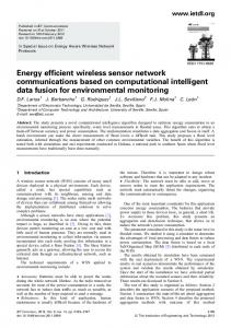
Fig. 2. CTP* does not distinguish between sleep and operation. It broadcasts regular beacons during maintenance (t < 0 s), even if neighbors are not yet available. The dashed line denotes the average over the last 10 s.
is detected, the node keeps listening, otherwise the radio is switched off immediately. This concept results in a very energy-efficient operation (duty cycle = Tcs /TP ), if there is no or little communication in the network. TP can be tuned for optimized energy consumption if channel utilization is known [9]. B. A Case for a Dedicated Maintenance Protocol In order to show the need for a protocol stack enhancement, we investigate the effect of maintenance on a state-of-the-art low-power protocol stack. In particular, we look at the start-up behavior of the TinyOS Collection Tree Protocol (CTP) on top of a LPL MAC protocol. The so-called CTP* [18] has been running efficiently and reliably on our testbed (cf. Sect. V-C) for months. CTP* does not feature a dedicated maintenance phase. Hence during the installation of the nodes, repeated neighbor announcements are broadcast long before all nodes are available. This results in an increased current draw of 0.67 mA during the installation of the nodes (cf. Fig. 2 for t < 0 s). As shown in Sect. VI-A a dedicated maintenance protocol such as NoSE reduces this amount by 60%. CTP* is designed and parameterized for an efficient overall operation, at the price of a delayed responsiveness during start. As shown in Fig. 3, CTP* shows a lot of parent switches, distributed throughout the network’s start-up. These switches can mostly be attributed to parent selections with bad link qualities and require a lot of control beacons for announcing the changes in the topology. The impact is two-fold: (1) it takes about an hour to build a stable topology and to conclude about the integrity of the network and (2) each control beacon wastes considerable energy as can be seen in a power trace in Fig. 2 for t ≥ 0 s. Using the NoSE protocol enhancement, the start-up process can be sped up and energy is saved due to the integrated link assessment of the NoSE discovery scheme. IV. N O SE IN D ETAIL Mode changes in NoSE are supported by an internal state machine depicted in Figure 1. Additional to the sleep and operational states, the transitional discovery state is responsible for the neighbor assessment. A mode change is initiated
Number of Parent Switches
50
30
the wake-up call. At any time, the operating network can be set back to sleep by flooding a sleep call in the network. An overview of all NoSE parameters and suggested setting is provided in Table I.
20
A. Network Calls
40
10 0
0
10
20
30
40 50 Duration [min]
60
70
80
Fig. 3. Dynamics of the network after start-up of CTP* in a 25-node testbed. It takes CTP* about an hour to obtain a stable topology.
by network calls: a wake-up call in sleep mode initiates an initialization of the network; a sleep call in operational state initiates the transition into a global, low-power-listening mode. On power-on, a node enters the very energy-efficient sleep state. While sleeping, the nodes only wake up every TPSleep for a quick poll of the channel. Since every node in the network follows this paradigm, no message exchange takes place during sleep. The sleep state is introduced in order to save energy after the node is initially powered on and during maintenance. In particular, it is of limited use to gather neighborhood information when not all surrounding nodes are yet available or nodes are added, removed and relocated. After installation or when the maintenance task is completed, the network is woken up by a wake-up call originating at a single node, e.g., the sink node. The wake-up call is disseminated by flooding the network. The flood notifies and synchronizes all nodes in the network for the upcoming quasisynchronous discovery phase by propagating two timer values: (1) the discovery start timer triggers the transition to the discovery state, (2) the discovery expiration timer triggers the exit from discovery (cf. Fig. 1). Quasi-synchronous in this respect means that the nodes synchronize on a common time window for the discovery phase. Hence a rather loose synchronization in the order of a second is sufficient. During discovery, an exhaustive neighbor search and link assessment is performed. All nodes send a predefined number of messages N , making it beneficial to decrease the channelpolling interval to TPDisc TPSleep .1 This shortens the duration of the discovery due to the temporarily increased bandwidth and saves considerable energy. The discovery phase ends at the same time for all neighbors. It results in complete and well-assessed neighbor information available at every node. On expiration of the discovery expiration timer, the node enters the operational phase. In particular, the nodes will first set up a network topology based on the well-assessed neighbor information provided by NoSE. For the operational state, the MAC’s polling interval is set to TPOp , which is propagated in 1 While non-duty cycled operation could be beneficial during discovery, we maintain LPL operation during all operational modes based on the requirement to have a single protocol stack and MAC layer.
Mode changes are initiated by network calls. These calls are triggered at a dedicated node (usually the sink) and flooded in the network. There are three possible network calls: (1) the wake-up call that wakes up the network, (2) the sleep call that puts the nodes back asleep and (3) the optional parameter call, which updates the MAC polling interval. A call comprises all information required for the subsequent mode transition: • It contains a call-type identifier, denoting whether the call is a sleep, wake-up or parameter call. • It contains a call id cid . For every new call initiated by the sink, the id is incremented. • It contains the countdown-timer TS , indicating the start time of the mode change, and its duration TD . • It includes two duty cycles for the MAC protocol. One is to be applied after the start of the mode change TS and the other one to be used after the expiration of the mode change TS + TD . The calls need to be reliable and fast in order to reach all nodes before the start of the discovery phase. Furthermore it is essential that calls induce only minimal overhead and are easily integrated. NoSE calls are based on a simple flood in the network. If a new call is received for the first time, a message is broadcast to all neighbors. Collisions are minimized by benefiting from the MAC’s collision avoidance, i.e., doing a carrier sense before sending. There is no need to use the NoSE specific wake-up call, if the system already provides means for a fast and reliable flood, e.g., Trickle [12]. A potential problem is if a node misses one of the calls flooded in the network. In order to ensure consistency in the network, NoSE calls provide a recovery scheme similar to the one of Trickle. Every node stores the most recent call ccur id . Whenever a call is received containing a newer call (cid > ccur id ), the call is forwarded and the old call is replaced in the history. Is the received call the node’s current call, the call is ignored. If the node however receives a call containing an old cur id (cid < ccur id ), the node broadcasts its state cid and hence ensures that the outdated node gets synchronized. Similar, if a node A receives a non-NoSE message during sleep from a node B, node A knows that the network is not consistent. It Parameter TS TD N TR TPSleep TPDisc TPOp
Description Remaining time until mode change Duration of mode change (discovery) Number of discovery packets Reserve time for queued packets (MAC) MAC polling interval during sleep MAC polling interval during discovery MAC polling interval when in operation
Typical Value 60 s 2 min 30 3s 1.5 s 50 ms 300 ms
TABLE I OVERVIEW OF N O SE PARAMETERS AND SUGGESTED SETTING .
therefore broadcasts its current state. Subsequently, node B A will get asleep if it had missed the sleep call, i.e., cB id < cid . B A Otherwise (cid > cid ) node B will send its current status, which indicates node A should become operational. 1) Wake-up Call: The wake-up call notifies and prepares all nodes in the network for the subsequent discovery phase. All nodes have to know the point in time TS when the discovery phase begins, its length TD , the number of packets N being exchanged and the channel-polling interval during discovery TPDisc and during the subsequent operational state TPOp . 2) Sleep Call: In the operational state, NoSE allows to set the network back asleep. This is done by flooding the network with a sleep call containing the duty cycle TPSleep during the sleep phase and the start time TS . The sleep phase lasts until receiving a wake-up call and hence has no duration (TD = 0). It is up to the application designer, whether the application should still gather new data and whether potentially buffered messages are to be forwarded should be kept in the queue or flushed. However, no messages are forwarded until the next time the operational state is entered. 3) Parameter Call: The parameter call is an optional feature of NoSE. It allows for adapting the MAC’s duty cycle. Similar to a wake-up call, the parameter call contains the time TS and the new duty cycle TPOp∗ . The start time TS ensures that all nodes in the network switch the duty cycle synchronously despite the propagation delay while flooding the call. Furthermore the parameter call allows to define a duration TD for which the new duty cycle should be applied before returning back to the old duty cycle. If the duration is set to zero, the duty cycle is changed to TPOp∗ upon further notice. Parameter calls do not trigger a mode state change. B. Discovery Phase The discovery phase starts at the same time for all nodes that have received the wake-up call. During discovery with duration TD the node sends exactly N broadcast messages containing their node identifier. In parallel to sending the broadcast messages, nodes keep a neighbor entry for all neighbors they receive packets from. In particular, they track the number of received packets and the maximum RSSI. As analyzed in a scenario without in-network interference [3], the number of received packets and the RSSI allows for reliably assessing the link quality. During the discovery, the network’s traffic is increased. This in turn will increase the probability for collisions that occur if broadcasts of different nodes (with length TPDisc ) partially overlap. By limiting the channel utilization CU , i.e., the fraction in time the channel is busy, the chances for collisions are reduced. The channel utilization CU depends on the number of neighbors L sending N messages each, the broadcast length TPDisc and the duration of the discovery TD : CU = N (L + 1)TPDisc /TD .
(1)
It is shown in Sect. VI-D that a CU of 0.2 should be chosen as an upper bound for the channel utilization in order to ensure
well-assessed link qualities. Collisions are further reduced at the MAC layer, which performs a carrier sense prior to the broadcast. If a carrier is detected, the packet is rescheduled with a short random backoff. Hence a packet may be delayed at the MAC layer for a short time before being transmitted. In order to account for this small possible delay, NoSE reserves a slot of length TR at the end of the discovery. During this reserved slot, the nodes must not schedule any broadcasts beforehand. This allows the MAC for transmitting broadcasts previously blocked by a positive carrier sense. The NoSE discovery messages are evenly distributed over the whole discovery phase. This avoids burst failures that are induced due to common short-time link failures in WNSs [3]. Hence, this even distribution of the discovery messages increases the fidelity of the link assessment. For this purpose, the discovery time is partitioned into N subslots. In each of the subslots the node selects independently a random time to send one discovery message. During discovery, NoSE shortens the channel-polling interval to TPDisc . According to Equation (1) this reduces the channel utilization CU and therefore allows reducing the discovery time TD . This shortening of the channel-polling interval increases the responsiveness and also saves sending energy in the order of TPSleep /TPDisc . V. I MPLEMENTATION AND T EST S ETUP A. Implementation NoSE has been implemented in TinyOS-2.x for Tmote Sky nodes, which feature a packet-based Chipcon CC2420 radio. We use the TinyOS-2.x CC2420 radio stack [19] with low power listening (LPL) enabled. NoSE is implemented as an individual layer in the protocol stack. Figure 4 shows NoSE integrated between the MAC and the Network layer. NoSE uses the standard MAC interface for transmitting its messages. We added an interface to adapt the polling interval TP on the fly. Furthermore the countdown-timer TS of the parameter call, which starts the subsequent mode change, is updated in the message buffer right before the call is forwarded. This allows for a synchronized mode-change. All NoSE packets (network calls and discovery packets) are identified using a user-defined frame type according to IEEE 802.15.4. Based on a received packet’s frame type, NoSE decides whether the packet needs to be internally handled or passed to the network layer. Internally, NoSE maintains a state machine containing three phases: sleep, discovery and operational (cf. Fig. 1). When the node is powered on, it switches into the energy-saving sleep state. As soon as a wake-up call is received, the node sets the discovery start and expiration timers. After the discovery phase, the node is in the operational state. In order to achieve a better fidelity in the link estimation, Chackeres et al. [20] showed that the discovery messages should have a similar packet size to the data messages being used during operation. NoSE therefore sends a discovery message with the same length as data messages sending additional information that can be used by the routing protocol, e.g., the node’s battery level.
D. Simulation
Network
NoSE
Block traffic outside operational phase Uses standard MAC interface for transmission
New interface Modify TP
LPL MAC
Fig. 4. NoSE stack. An interface allowing for runtime modification of TP is provided.
B. Integration After the discovery, the collected neighbor information has to be transferred to the routing protocol. Thus, it is advisable that NoSE and the routing protocol share a neighbor list. As an example, consider the widely used ETX [21] routing scheme, where packets are routed based on the overall link performance of routes. This requires knowledge on each link’s PPR, which can be gained directly from the link-assessment information collected during NoSE’s discovery phase. This results in a great performance gain compared to the current TinyOS 2.x ETX implementation, where all links are initialized as being perfect (EETX = 0, as of revision 1.4). C. Testbed Evaluation NoSE is designed to improve the effectiveness of real deployments. To this end, we tested NoSE in a realistic environment. The application scenario assumed is a wireless multi-hop fire-detection network initialized with NoSE. The nodes’ neighbor density and location is characteristic for firedetectors deployed in an office building: 25 nodes deployed over several offices on a single floor. The average neighbor density is 7.4; the maximum density is 12. For the evaluation, 558 test runs were performed. In order to check the quality of NoSE’s neighbor search, it is required to have a profound knowledge of the network characteristics, i.e., all neighbors and the according link qualities. This information however is susceptible to change. For this reason, the network characteristics have been measured 18 times over a period of six weeks, alternating with the performance evaluation of the NoSE protocol. For each assessment, every node sent 1000 broadcast messages (with a length in the order of 1 ms) randomly distributed over a period of three hours using CSMA without duty cycling. We extract two different metrics from this reference data, which are used in the evaluation: the Packet Reception Rate (PRR) and the Long Term PRR (LTPRR). The term PRR reflects a single link assessment being closest in time to the NoSE test. The LTPRR expresses the link performance over the whole six weeks, i.e., over all 18 link measurements. Furthermore, the terminology High-Quality Links, refers to links with a (LT)PRR > 95%.
In order to show the scalability of the discovery, NoSE has also been simulated in Castalia 1.3, a state-of-the-art WSN simulator based on OMNet++. Castalia provides a realistic wireless channel model that captures the effects of the so called grey area. As with real deployments, this model results in many links that exhibit poor performance. Castalia calculates packet collisions based on the signal-to-interferenceplus-noise ratio. Castalia further provides a radio model that features transition times between the radio’s states. Our radio model specifically uses the characteristics of the CC2420 to match the testbed evaluation. The simulations use a network containing 160 nodes, arranged in a grid with a small Gaussian-distributed displacement. The network represents an event-detection system where nodes are rather evenly spread. The grid size is varied resulting in node densities ranging from 4 to 45 neighbors. 60 different topologies were analyzed by feeding random seeds to the grid’s displacement and the wireless channel model. VI. P ERFORMANCE E VALUATION The metrics used to benchmark NoSE evaluate the major concerns for the maintenance: (1) energy efficiency, (2) responsiveness and integration and (3) the completeness of the neighbor search and the quality of the link assessment. These metrics are evaluated based on the most important maintenance task: the original deployment of the nodes and the subsequent first start of the application. It is essential that the node’s energy consumption is minimized during the deployment, yet shows a fast and reliable start-up as soon as all nodes in the network are installed. It should be noted that the analyzed deployment and first start-up show very similar characteristics to other subsequent maintenance tasks. Focusing on the initialization, NoSE can be compared to the Birthday Protocol (BP) [14]. While BP neither features operational mode changes nor link assessment during initialization, we can compare NoSE based on energy efficiency and responsiveness during the initialization. BP has been implemented according to the protocol description in [14] and evaluated with the suggested parameter allowing to find 95% of the available links. Concerning integration, NoSE is designed to easily integrate with the predominantly used LPL MAC protocols. On the other hand, BP requires a separate, second radio stack. A. Energy Efficiency during Deployment The energy consumption is analyzed by measuring a single node’s power consumption. Fig. 5 displays the traces of the two protocols’ power consumption during the deployment and the start-up phase. Power measurements are performed with an Agilent N6705A power analyzer, with a sample time of 1 ms. For illustration purposes, samples are integrated and plotted over periods of 100 ms each. During the deployment of the nodes, drastic power savings have a significant impact when the installation time is in the order of days. Fig. 5 only presents the last 100 s
25 −∞ → Deployment
Wake−up
25
+∞ →
Discovery
−∞ → Deployment
Current [mA]
Current [mA]
15 10
15 10 5
5 0 −100
Discovery → ∼600s
20
20
−50
0
50 Time [s]
100
150
200
(a) NoSE is energy-efficient and finishes within a given time.
0 −100
−50
0
50 Time [s]
100
150
200
(b) BP is less energy-efficient and non-deterministic.
Fig. 5. Measured current consumption and responsiveness analysis for NoSE and BP during initialization in the testbed. The dashed line indicates the average energy consumption of the different protocol states.
Energy Consumption [mAh]
250 200
B. Responsiveness
TinyOS (CTP*) Birthday NoSE
150 100 50 0 0
Fig. 6.
5 10 Deployment Duration [days]
15
Extrapolated energy consumption comparison during initialization.
of the deployment phase, whereas this phase usually takes orders of magnitudes longer for real installations (i.e., days). Nevertheless, longer measurements confirmed that these trace excerpts are representative for the node’s behavior. NoSE’s deployment (sleep) phase shows a very regular and lowpower consumption, with an average current drain of 0.28 mA. This is due to NoSE’s low duty cycle merely sampling the channel once every second. BP following the same paradigm of listening only, shows an increased current drain of about 0.41 mA. This can be attributed to a rather long channel sampling time of 20 ms waiting for a message to be received. Another interesting artifact can be seen around the interval -70 to -50 s, where BP did not sample the channel for about 20 s. Due to the use of random sampling times, nodes may sporadically stop to listen to the channel for a long time, rendering the protocol highly non-deterministic. Fig. 6 shows the significant energy savings when using a dedicated maintenance scheme compared to the standard routing protocol CTP*. For the comparison, it should be stressed that both NoSE and CTP* are based on the same LPL MAC protocol. CTP* requires 115 mAh over a period of 7 days and hence 5% of the available energy of a single alkaline AA battery (2200 mAh). The dedicated sleep phase of NoSE allows to reduce this amount by 60%.
The second important metric is the responsiveness of the start-up. This is shown in Fig. 5, where t = 0 s indicates the begin of the start-up. BP’s runtime is non-deterministic. In particular the start time of the discovery differs for all nodes in the network. As illustrated in Fig. 5(b), the node started its discovery at t = 62 s. Hence the node initiating the discovery at t = 0 s had already finished its discovery. NoSE on the other hand features a deterministic start-up time, which is controllable by an application-specific length of wake-up and discovery. Minimizing these two phases directly increases the responsiveness. NoSE’s wake-up call is evaluated for reliability and speed. Only in one out of the 558 runs on the testbed, the wakeup call was not received by all nodes. The nodes were always notified within less than 20 s. Nevertheless a pessimistic wakeup period of TS = 60 s is chosen and allows for flexibility in the network size. For the discovery phase, a period of 1 to 2 minutes has shown to be an adequate value (cf. Sect. VI-D). Overall NoSE provides well-assessed neighborhood information in just about 3 minutes starting from a wake-up call. BP and NoSE both require knowing the end time of the discovery phase, which allows for switching to operational mode, e.g., to set up the routing tables. For BP, this requires estimating the discovery’s runtime, which is upper bounded by the network’s diameter multiplied by the discovery time. Hence a conservative estimate of the a priori unknown diameter of the network has to be made. NoSE on the other hand features a bounded and deterministic duration of the discovery phase, allowing for a smooth transmission to the subsequent operation. C. Neighbor Discovery: NoSE vs. BP The initialization schemes of NoSE and BP both provide a neighbor discovery, which we compare in the following. NoSE and BP both aim at finding all available neighbors. Table II shows their success rate, each sending 20 discovery broadcasts. The table segments the number of found neighbors according the measured link quality (PRR). Both protocols find almost all of the available high-quality links. The same holds for links
≥ 95 155 97.8% 97.0%
PRR [%] #Links NoSE BP
85 − 95 45 88.8% 91.9%
50 − 85 42 80.8% 82.5%
< 50 75 59.3% 70.4%
TABLE II C OMPARISON OF THE NEIGHBOR DISCOVERY PERFORMANCE MEASURED IN THE TESTBED . B OTH PROTOCOLS FIND ALMOST ALL HIGH - QUALITY LINKS , BUT ALSO A SUBSTANTIAL NUMBER OF LOW- QUALITY LINKS .
thumb, for every 10 messages being sent, the discovery should last an additional minute. For instance, 50 messages require 5 min for finding most LTPRR links. Having a channel-polling interval TPDisc = 100 ms and a maximal number of neighbors of L = 12 in our testbed, the maximal channel utilization CU should be: CU ≤ N (L + 1)TPDisc /TD = 10(12 + 1)0.1/60 ≈ 0.2 (2)
100
A unique feature of NoSE is its integrated link assessment. The assessment is based on the knowledge that all nodes in the network send N discovery messages. Based on the number of messages a node receives from a specific neighbor, it assesses the link quality. This assumption implies that discovery messages are lost due to bad links and not due to collisions and requires to limit the channel utilization factor CU according to Equation (1). Subsequently an upper bound for CU is determined. The influence of collisions on the link estimation is analyzed in Fig. 7 showing the number of high-quality (LTPRR) links, which received at least 90% of the messages. As a rule of
In this paper we have addressed the issue of maintenance in a Wireless Sensor Network deployment. We presented NoSE, a protocol stack enhancement allowing for mode changes of a network while under operation. This allows switching the network into an energy-efficient sleep state while maintenance is being performed. It further allows for the possibility to switch a network off, if the data from the network is temporarily not being used. NoSE is readily usable with LPL MAC protocols commonly used today. NoSE utilizes resources effectively, switching to high bandwidth phases where necessary, but drastically constraining
#Discovered HQ links (LTPRR) [%]
D. NoSE: Link-Assessment Quality
Hence, the discovery duration can be almost arbitrarily reduced by shortening the polling interval TPDisc . However, this reduction of the discovery phase also shortens channelassessment time. As shown in [3] (in an office environment with Tmote Sky nodes), the link estimation is susceptible to short-term link fluctuations if the message interval undercuts two seconds. Hence, if the link assessment quality is of paramount importance, the discovery time TD for this configuration should not fall below 2 · N seconds. In order to show the scalability of NoSE’s discovery scheme, the effect of different network densities is simulated. Fig. 8 shows the performance of the link assessment in simulation depending on the node density, highlighting the fraction of collisions for high-quality links. Identical to the testbed results, a highly increased bandwidth jeopardizes the link assessment. If the data load is low, e.g., 10 messages in 2 min as seen in Fig. 8(a), the number of collisions are limited to about 4%, even with 45 neighbors. More detailed, for a discovery duration of 120 s, Fig. 8(b) shows an increased number of lost packets for more than 11 neighbors. This is identical to the implementation results, emphasizing that a channel bandwidth of 20% must not be exceeded during discovery. Thus, the discovery phase can be tuned for an optimized performance by estimating the deployment’s maximal node density. For parameterizing the discovery, it has to be decided how solid the links should be assessed. Is a link estimation based on N = 10 messages sufficient or should rather N = 50 messages be sent? The discovery time should then be set to about TD = 2 · N seconds as discussed above. For setting the appropriate channel polling time, an estimate of the maximal number of neighbors L in the network has to be made and results in TPDisc ≤ 0.4/(L + 1) according to Equation (2). For a typical scenario of initializing a WSN, Table I details on the suggested settings of NoSE’s parameters.
Fig. 7. NoSE discovery phase on testbed: A high channel utilization CU , i.e., N large and TD short, jeopardizes the link assessment.
with a link quality of 85-95%. However, both protocols also find a substantial number of links, with a poor link quality. These links should not be included, emphasizing the necessity of a link assessment prior to setting up of the routing tables. During discovery, both protocols show an increased activity. Even though discovery time is short, the energy consumption requires considerations: In BP (cf. Fig. 5(b) between t = 62 s and t = 122 s) the radio is always turned on, running with a 100% duty cycle. NoSE uses the low-power mechanism of the MAC, allowing for a reduced energy consumption as indicated in Fig. 5(b). Despite the increased activity during the discovery, NoSE allows for a reduced duty cycle of less than 20% for the same duration of 1 min as the Birthday’s discovery phase, thus being 5 times as efficient. BP’s non-deterministic behavior, the requirement of a second radio stack and the lack of an integrated link-quality estimation show its limited usability when being integrated into a system.
Fig. 8. NoSE discovery phase in simulation. The parameters need to be adapted to the network density in order to ensure well assessed links (TPDisc = 100 ms).
power consumption otherwise. It manages the trade-off between optimal responsiveness required and an efficient, minimal usage of the energy resource. Furthermore NoSE offers superior solutions for initialization that outperform standard and specialized approaches by at least 30% energy savings during maintenance. A chief aspect of NoSE is its bounded operation time, which allows for timely validation of system operation. Additionally, NoSE’s unique integration of link estimation allows for a well-assessed neighborhood. By filtering out mediocre links, NoSE increases the stability and performance of the networking phase in the operational state. ACKNOWLEDGMENT The work presented in this paper was supported by CTI grant number 8222.1 and the National Competence Center in Research on Mobile Information and Communication Systems (NCCR-MICS), a center supported by the Swiss National Science Foundation under grant number 5005-67322. R EFERENCES [1] N. Burri, P. von Rickenbach, and R. Wattenhofer, “Dozer: ultra-low power data gathering in sensor networks,” in Proc. 6th Int’l Conf. Information Processing Sensor Networks (IPSN ’07). New York, NY, USA: ACM Press, Apr. 2007, pp. 450–459. [2] K. Srinivasan and P. Levis, “RSSI is under appreciated,” in Proc. 3rd IEEE Workshop on Embedded Networked Sensors (EmNetS-III), May 2006. [3] A. Meier, T. Rein, J. Beutel, and L. Thiele, “Coping with unreliable channels: Efficient link estimation for low-power wireless sensor networks,” in Proc. 5th Int’l Conf. Networked Sensing Systems (INSS 2008). Kanazawa, Japan: IEEE, Jun. 2008, pp. 19–26. [4] T. L. Dinh, W. Hu, P. Sikka, P. Corke, L. Overs, and S. Brosnan, “Design and deployment of a remote robust sensor network: Experiences from an outdoor water quality monitoring network,” in Local Computer Networks, 2007. LCN 2007. 32nd IEEE Conference on, Oct. 2007, pp. 799–806. [5] W. Ye, F. Silva, and J. Heidemann, “Ultra-low duty cycle mac with scheduled channel polling,” in Proc. 4th ACM Conf. Embedded Networked Sensor Systems (SenSys 2006). New York, NY, USA: ACM Press, 2006, pp. 321–334. [6] L. v. Hoesel and P. Havinga, “A lightweight medium access protocol (LMAC) for wireless sensor networks,” in Proc 1st Int’l Workshop Networked Sensing Systems (INSS04), Tokyo, Japan, Jun. 2004. [7] G. Halkes and K. Langendoen, “Crankshaft: An energy-efficient MACprotocol for dense wireless sensor networks,” in Proc. 4th European Workshop on Sensor Networks (EWSN 2007), ser. Lecture Notes in Computer Science, vol. 4373. Delft, The Netherlands: Springer, Berlin, Jan. 2007, pp. 276–290.
[8] J. Hill and D. Culler, “Mica: A wireless platform for deeply embedded networks,” IEEE Micro, vol. 22, no. 6, pp. 12–24, Nov. 2002. [9] J. Polastre, J. Hill, and D. Culler, “Versatile low power media access for wireless sensor networks,” in Proc. 2nd ACM Conf. Embedded Networked Sensor Systems (SenSys 2004). ACM Press, New York, 2004, pp. 95–107. [10] A. El-Hoiydi and J. Decotignie, “WiseMAC: An ultra low power MAC protocol for multi-hop wireless sensor networks,” in Proc. 1st Int’l Workshop Algorithmic Aspects of Wireless Sensor Networks (ALGOSENSORS 2004), ser. Lecture Notes in Computer Science, S. Nikoletseas and J. Rolim, Eds., vol. 3121. Springer, Berlin, Jun. 2004, pp. 18–31. [11] J. Hui and D. Culler, “The dynamic behavior of a data dissemination protocol for network programming at scale,” in Proc. 2nd ACM Conf. Embedded Networked Sensor Systems (SenSys 2004). ACM Press, New York, Nov. 2004, pp. 81–94. [12] P. Levis, N. Patel, D. Culler, and S. Shenker, “Trickle: A self-regulating algorithm for code propagation and maintenance in wireless sensor networks,” in Proc. First Symp. Networked Systems Design and Implementation (NSDI ’04). ACM Press, New York, Mar. 2004, pp. 15–28. [13] R. Musaloiu-E., C.-J. M. Liang, and A. Terzis, “Koala: Ultra-low power data retrieval in wireless sensor networks,” in IPSN ’08: Proceedings of the 7th international conference on Information processing in sensor networks. Washington, DC, USA: IEEE Computer Society, 2008. [14] M. J. McGlynn and S. A. Borbash, “Birthday protocols for low energy deployment and flexible neighbor discovery in ad hoc wireless networks,” in Proc. 2nd ACM Int’l Symp. Mobile Ad Hoc Networking and Computing (MobiHoc 2001). New York, NY, USA: ACM Press, 2001, pp. 137–145. [15] F. Kuhn, T. Moscibroda, and R. Wattenhofer, “Initializing newly deployed ad hoc and sensor networks,” in Proc. 10th ACM/IEEE Ann. Int’l Conf. Mobile Computing and Networking (MobiCom 2004). ACM Press, New York, 2004, pp. 260–274. [16] T. Moscibroda, P. von Rickenbach, and R. Wattenhofer, “Analyzing the energy-latency trade-off during the deployment of sensor networks,” in Proc. 25th Ann. Joint IEEE Conf. Computer Communication Soc. (Infocom 2006), Apr. 2006. [17] A. Woo, T. Tong, and D. Culler, “Taming the underlying challenges of reliable multihop routing in sensor networks,” in Proc. 1st ACM Conf. Embedded Networked Sensor Systems (SenSys 2003). New York, NY, USA: ACM Press, 2003, pp. 14–27. [18] R. Lim, M. Woehrle, A. Meier, and J. Beutel, “Poster abstract: Harvester - low-power environment monitoring out of the box,” in Proc. 6th European Workshop on Sensor Networks (EWSN 2009). Cork, Ireland: Springer, Feb. 2009. [19] D. Moss, J. Hui, and P. Levis, “TinOS 2.x, TEP 126 – CC2420 Radio Stack,” TinyOS Developer List, Mar. 2007. [20] I. D. Chakeres and E. M. Belding-Royer, “The utility of hello messages for determining link connectivity,” in Proc. 5th Int’l Symp. Personal Wireless Multimedia Communications (WPMC 2002), vol. 2, Oct. 2002, pp. 504–508. [21] D. S. J. D. Couto, D. Aguayo, J. Bicket, and R. Morris, “A highthroughput path metric for multi-hop wireless routing,” Wireless Networks, vol. 11, no. 4, pp. 419–434, 2005.