data. In this paper, we propose an efficient algorithm, called HI-mine, based on a new data structure, called HI-struct, for mining the complete set of indirect associations ...... Using SAS for Mining Indirect Associations in. Data, In Proc of the ...
Efficient Mining of Indirect Associations Using HI-Mine Qian Wan and Aijun An Department of Computer Science, York University Toronto, Ontario M3J 1P3 Canada {qwan, aan}@cs.yorku.ca
Abstract. Discovering association rules is one of the important tasks in data mining. While most of the existing algorithms are developed for efficient mining of frequent patterns, it has been noted recently that some of the infrequent patterns, such as indirect associations, provide useful insight into the data. In this paper, we propose an efficient algorithm, called HI-mine, based on a new data structure, called HI-struct, for mining the complete set of indirect associations between items. Our experimental results show that HI-mine's performance is significantly better than that of the previously developed algorithm for mining indirect associations on both synthetic and real world data sets over practical ranges of support specifications.
1
Introduction
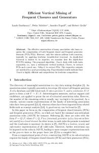
Since it was first introduced by Agrawal et al. [4] in 1993, association rule mining has been studied extensively by many researchers. As a result, many algorithms have been proposed to improve the running time for generating association rules and frequent itemsets. The latest includes FP-growth [6], which utilizes a prefix-tree structure for compactly representing and processing pattern information, and H-mine [8], which takes advantage of a novel hyper-linked data structure and dynamically adjusts links in the mining process. While most of the existing algorithms are developed for efficient mining of frequent patterns, it has been noted recently that some of the infrequent patterns may provide useful insight into the data. In [13], a new class of patterns called indirect associations has been proposed and its utilities have been examined in various application domains. Consider a pair of items, x and y, that are rarely present together in the same transaction. If both items are highly dependent on the presence of another itemsets M, then the pair (x, y) is said to be indirectly associated via M. Fig. 1 illustrates a high-level view of an indirect association. There are many advantages to mining indirect associations in large data sets. For example, an indirect association between a pair of words in text documents can be used to classify query results into categories [13]. For instance, the words coal and data can be indirectly associated via mining. If only the word mining is used in a query, documents in both mining domains are returned. Discovery of the indirect association between coal and data enables us to classify the retrieved documents into
coal mining and data mining. There are also potential applications of indirect associations in many other real-world domains, such as competitive product analysis and stock market analysis [13]. infrequent
frequent x
frequent M
y
Fig. 1. Indirect association between x and y via mediator M
For mining indirect associations between itempairs, an algorithm is presented in [11, 13]. There are two phases in the algorithm: 1. Extract all frequent itemsets using standard frequent itemset mining algorithms such as Apriori [3] or FP-growth [6]; 2. Discover valid indirect associations by checking all the candidate associations generated from the frequent itemsets. In this paper, we propose a new data structure, HI-struct, and a new mining algorithm, HI-mine, for mining indirect associations in large databases. We show that they can be used as a formal framework for discovering indirect associations directly, with no need to generate all frequent itemsets as the first step. Empirical evaluations comparing HI-mine to two versions of the algorithm described above show that HImine performs significantly better on both synthetic and real world data sets. The remaining of the paper is organized as follows. Section 2 reviews related work and briefly exhibits the contribution of the paper. Next, we present the HI-struct data structure and the HI-mine algorithm in Section 3. Our empirical results are reported in Section 4. Finally, we conclude with a summary of our work and suggestions for future research in Section 5.
2
Related Work
Let I = {i1, i2,…, im} be a set of m literals, called items. Let the database D = {t1, t2,…, tn} be a set of n transactions, each one consisting of a set of items from I and associated with a unique identifier called its TID. The support of an itemset A is the percentage of transactions in D containing A: sup(A) = ||{t | t ∈ D, A ⊆ t}|| / ||{ t | t ∈ D}||, where ||X|| is the cardinality of set X. An itemset is frequent if its support is more than a user-specified minimum support value.
2.1
Negative Association Rules
B is a conditional implication among itemsets A and B, An association rule A where A ⊂ I, B ⊂ I and A ∩ B = ∅. The confidence of an association rule r: A B is the conditional probability that a transaction contains B, given that it contains A. The support of rule r is defined as: sup(r) = sup(A∪B). The confidence of rule r can be expressed as conf(r) = sup(A∪B)/sup(A). The importance of extending the current association rule framework to include negative association was first pointed out in [5]. In the case of negative association rules we are interested in finding itemsets that have a very low probability of occurring together. That is, a negative association between two itemsets A and B, denoted as A B or A B , means that A and B appear very rarely in the same transaction. Mining negative association rules is impossible with a naïve approach because billions of negative associations may be found in a large dataset while almost all of them are extremely uninteresting. This problem was addressed in [14] by combining previously discovered positive associations with domain knowledge to constrain the search space such that fewer but more interesting negative rules are mined. �
2.2
�
Indirect Association and INDIRECT Algorithm
Indirect association is closely related to negative association, they are both dealing with itemsets that do not have sufficiently high support. Indirect associations provide an effective way to detect interesting negative associations by discovering only “infrequent itempairs that are highly expected to be frequent” without using negative items or domain knowledge. Definition 1 (Indirect Association) An itempair {x, y} is indirectly associated via a mediator M, if the following conditions hold: 1. sup({x, y}) < ts (Itempair Support Condition) 2. There exists a non-empty set M such that: (a) sup({x} ∪ M) ≥ tf, sup({y} ∪ M) ≥ tf (Mediator Support Condition) (b) dep({x}, M) ≥ td, and dep({y}, M) ≥ td, where dep(P, Q) is a measure of the dependence between itemsets P and Q. (Mediator Dependence Condition) The thresholds above are called itempair support threshold (ts), mediator support threshold (tf), and mediator dependence threshold (td), respectively. In practice, it is reasonably to set tf ≥ ts. In the database and probability theories, an indirect association is a well-know property of embedded multi-valued dependency (EMVD) and probability conditional independence, where it is sometimes called an “induce dependence”. [16] includes a comprehensive discussion on an independence in a small context becoming a dependence in a larger context in both the database and probability settings. In this paper, we use the notation to represent the indirect association between x and y via M. And we use the IS measure [10] as the dependence measure
for Condition 2(b). Given a pair of itemsets, say X and Y, its IS measure can be computed using the following equation: IS ( X , Y ) ≡
P ( X ,Y ) P ( X ) P (Y )
(1)
where P denotes the probability that the given itemset appears in a transaction. An algorithm for mining indirect associations between pairs of items is given in [11, 13], which is shown in Figure 2. There are two major phases in this algorithm: (1) extract all frequent itemsets using Apriori (step 1) and (2) discover all indirect associations by (a) candidate generation (step 4) and (b) candidate pruning (steps 58). In the candidate generation step, frequent itemset Lk is used to generate candidate indirect associations for pass k+1, i.e., Ck+1. Each candidate in Ck+1 is a triplet, , where x and y are the items that are indirectly associated via the mediator M. Ck+1 is generated by joining the frequent itemsets in Lk. During the join, a pair of frequent k-itemsets, {x1, x2, …, xk} and {y1, y2, …, yk}, are joinable if the two itemsets have exactly k-1 items in common and thus produce a candidate indirect association , where x and y are the distinct items, one from each k-itemset, and M is the set of common items. For example, two frequent itemsets, {a, b, c, d} and {a, b, d, e}, can be joined together to produce a candidate indirect association, . Since the candidate associations are created by joining two frequent itemsets, they all satisfy the mediator support condition. Therefore, in the steps for candidate pruning, only itempair support condition and mediator dependence condition are checked. 1.
Extract frequent itemsets, L1, L2,…Ln, using frequent itemsets generation algorithm, where Li is the set of all frequent i-itemsets. 2. P = ∅ (set of indirect associations) 3. for k = 2 to n do 4. Ck+1 = join(Lk, Lk) 5. for each < x, y , M> ∈ Ck+1 do 6. if (sup({x, y}) < ts and dep({x}, M) ≥ td and dep({y}, M) ≥ td) 7. P = P ∪ {< x, y , M>} 8. end 9. end 10. end
Fig. 2. The INDIRECT algorithm
There are two join steps in the INDIRECT algorithm. One is in the first phase for generating all the frequent itemsets with Apriori. In Apriori, the join operation is used to generate candidate frequent itemsets for pass k+1 based on the frequent itemsets in Lk. The other join operation is for generating candidate indirect associations, Ck+1, from Lk. Both candidate generation steps can be quite expensive, because each of them requires at most O( k |Lk| × |Lk|) join operations. The join operation for generating indirect association candidates is more expensive than that in Apriori because the items in an indirect itempair, x and y, do not have to be the last item in each frequent itemset, whereas Apriori only combines itemsets that have identical k-1 prefix items, assuming that all the items in an itemsets are sorted in lexicographic
order. Moreover, no matter what implementation technique is applied, an Apriori-like algorithm may still suffer from nontrivial costs in situations with prolific frequent patterns, long patterns, or quite low minimum support thresholds. Is there any other way that we may reduce these costs in indirect association mining? Can we avoid generating all the frequent itemsets and a huge set of candidates, and derive indirect association directly using some novel data structure or algorithm? In the next section, we introduce our solution. The solution is based on the HIstruct data structure and the HI-mine algorithm, which were inspired by a novel hyper-linked data structure, H-struct, and an efficient algorithm, H-mine, presented in [8]. H-struct and H-mine are designed for the purpose of mining frequent patterns. We modify both of them for learning indirect association. With HI-struct and HImine, we do not need to find all the frequent itemsets before mining indirect associations nor we need to do any join operation for candidate generation. Instead we generate two new sets: indirect itempair set and mediator support set by recursively building the HI-struct data structures for the database. Then indirect associations are discovered from these two sets directly and efficiently.
3 Mining Indirect Association Using HI-mine In this section, we first define indirect itempair set (IIS) and mediator support set (MSS). We then illustrate the general idea of HI-mine (Hyper-structure Indirectassociation Mining) using the two sets with an example. Definition 2 (Indirect Itempair Set) Let ts be the itempair support threshold and L be the set of frequent itemsets of a database D with respect to ts. We define the indirect itempair set IIS of D as: IIS(D) = { | {x} ∈ L, {y} ∈ L, and sup({x, y}) < ts} Definition 3 (Mediator Support Set) Let L be the set of frequent itemsets of a database D. Let tf be the mediator support threshold and td be the mediator dependence threshold. The mediator support set MSS of x ({x} ∈ L) is defined as: MSS(x) = {M | M ∈ L, sup(M ∪ {x}) ≥ tf, and dep(M, {x}) ≥ td} It’s trivial to prove that the following properties hold for each indirect association of database D: 1. ∈ IIS(D); 2. M ∈ MSS(x) and M ∈ MSS(y). And on the other hand, given x, y and M that have the above properties, must be an indirect association of D.
3.1
HI-struct: Design and Construction
The design and construction of HI-struct for efficient indirect association mining are illustrated in the following example. The original transaction database TDB is shown in Table 1. The HI-struct of TDB is a dynamic data structure that changes during the process of recursively generating the indirect itempair set and mediator support sets. TID T100 T200 T300 T400 T500 T600 T700 T800
List of item_IDs A, B, C, D A, B, E, F G, H B, C A, B, D, E, I B, C, D J, K L, M, N
Table 1. The transaction database TDB
The initial HI-struct is constructed in the following steps. 1. Scan the transaction database TDB once. Collect the set of frequent items F and their supports. Sort F in support descending order as L, the list of sorted frequent items. For the example database, L is {B, A, C, D, E}. Then a header table H is created, where each frequent item has an entry with three fields: an item-id, a support count, and a pointer to a queue. 2. For each transaction Trans in TDB, select and sort the frequent items in Trans according to the order of L. Let the sorted frequent item list in Trans be [t|T], where t is the first element and T is the remaining list. [t|T] is called the frequent-item projection of transaction Trans. Add [t|T] to a frequent-item projection array, and append [t|T]’s index of the array to t’s queue. Thus, all indexes of the frequent-item projections with the same first item (in the order of L) are linked together as a queue, and the entries in the header table H act as the heads of the queues. Header Table of TDB B 5 A 3 C 3 D 3 E 2
1 2 3 4 5
Frequent-Item Projection 1 B,A,C,D 2 B,A,E 3 B,C 4 B,A,D,E 5 B,C,D
Fig. 3. The initial HI-struct of TDB
The initial HI-struct of the example database is shown in Figure 3. Since all frequent item projections in our example database start with B, the queues for other
items than B are empty at the moment1. After the initial HI-struct is constructed, the remaining mining process is performed on the HI-struct only, without referencing any information in the original database. Note that the frequent-item projection array contains only frequent items. Its size is usually much smaller than the original database. Therefore, the array may fit into main memory. The subsequent mining process involves building the indirect itempair set (IIS) of the database and the mediator support set (MMS) of each frequent item. We use a divide-and conquer strategy to build IIS and each MMS by partitioning each set into disjoined subsets and generating each subset in turn. Following the support descending order of frequent items: B, A, C, D, E, the complete indirect itempair set and mediator support sets of all the frequent items in our example database can be partitioned into 5 subsets as follows: (1) those containing item B; (2) those containing item A but no item B; (3) those containing item C, but no item B nor A; (4) those containing item D, but no item B nor A nor C; (5) those containing only item E. Clearly, all the frequent-item projections containing item B, referred to as the Bprojected database, are already linked in the B-queue in the header table, which can be traversed efficiently. In the next section, we will show that, by mining the Bprojected database recursively, HI-mine can find the indirect itempair set and mediator support sets (MSS) of all the frequent items in the first subset, i.e., all the indirect itempairs and support mediators containing item B. After that, each index in B-queue is added to the queue for the next item in the corresponding projection following B in the order of L to mine all the indirect itempair set and mediator support sets containing item A but not B. The HI-struct after this adjustment is shown in Figure 4. Note that B-queue is no longer needed and is thus removed. After the subsets containing A but not B are mined, other subsets of indirect itempair set and mediator support sets are mined similarly. Header Table of TDB B 5 A 3 C 3 D 3 E 2
1 2 4 3 5
Frequent-Item Projection 1 B,A,C,D 2 B,A,E 3 B,C 4 B,A,D,E 5 B,C,D
Fig. 4. HI-struct of TDB after mining B-projected database
3.2
HI-mine Algorithm
The HI-mine algorithm mines the complete set of indirect associations based on a dynamically-changed HI-struct. There are two phases in the algorithm. In the first phase, we construct HI-struct and generate the indirect itempair set of the database and mediator support set of each frequent item. In the second phase, we generate all 1
The initial header table of a database may contain more than one queue. We use a simple example for the convenience of explanation.
the indirect associations based on the indirect itempair set and the mediator support sets. The algorithm is described as follows. Algorithm: HI-mine. (Mine indirect associations using an HI-struct) Input: A transaction database (D); itempair support threshold (ts); mediator support threshold (tf); mediator dependence threshold (td); Output: The complete set of indirect associations between itempairs. Method: 1. build the initial HI-struct for D which includes a header table H and the frequent item projection array. 2. for each item i in the header table of HI-struct 3. create header table Hi by scanning i-projected database in the same way as building header table H except that item i is not considered (see Figures 5, 10 - 13) 4. hi_mine(Hi) 5. insert all the indexes in i-queue to the proper queues in H (see Figure 4) 6. end 7. if IIS(D) ≠ ∅ then 8. for each itempair in IIS(D) 9. SM ← MSS(x) ∩ MSS(y) 10. if SM ≠ ∅ 11. for each mediator M in SM 12. output 13. end 14.else 15. output “Indirect associations do not exit in this database” 16.end procedure hi_mine(Hm) (Recursively mine the header table of itemset m and update IIS(D) and MSS(j), j ∉ m) 1. for each item j in the header table Hm 2. if j's count > minimum mediator support count then 3. if IS(j, m) > td then 4. add m to MSS(j) 5. create header table Hmj by scanning j-queue in Hm (i.e., mj-projected database) in the same way as building H except that item j and items in m are not considered (see Figure 7) 6. hi_mine(Hmj) 7. else if the size of m is 1 and j's count < minimum itempair support count then 8. add to IIS(D) 9. end 10. insert all the indexes in j-queue to the proper queues in Hm (see Figure 6) 11.end Figures 5 to 13 show the execution of the algorithm on the transaction database TDB given in Table 1. The itempair support threshold ts and mediator support
threshold tf are set to be 25% (minimum support count and minimum mediator support count are both 2)2, and the minimum dependence threshold td is 0.5. First, to find all the indirect itempairs and support mediators containing item B, a B-header table HB is created, as shown in Figure 5. In HB, every frequent item, except for B itself, has an entry with the same fields as H, i.e., item-id, support count and a pointer to a queue. The support count in HB records the support of the corresponding item in the B-queue. For example, since item A appears 3 times in the frequent-item projections of B-queue, the support count in the entry for A in HB is 3.
Header Table of {B:5} A 3 C 3 D 3 E 2
IIS(TDB) = ∅ MSS(A) = {{B}} MSS(C) = {{B}} MSS(D) = {{B}} MSS(E) = {{B}}
1 2 4 3 5
Fig. 5. Header table HB and mining result
By traversing the B-queue once, the set of locally frequent items, i.e., the items appearing at least 2 times, in the B-projected database is found, which is {A, C, D, E}. Since all the items in HB are locally frequent, there is no indirect itempair contains item B, and IIS(D) is empty after this scan. Because the minimum mediator support count is 2, we compute the IS measure between B and each item in HB: IS ({B}, { A}) = 3
3 × 5 = 0.77
(2)
IS ({B}, {C}) = 3
3 × 5 = 0.77
(3 )
IS ({B}, {D}) = 3
3 × 5 = 0.77
(4 )
IS ({B}, {E}) = 2
2 × 5 = 0.63
(5 )
They all pass the minimum dependence threshold 0.5. Therefore, {B} should be in the MMS of each of these items. The result is shown in Figure 5. After {B} is inserted into MSS(A) in the above process, a header table HBA is created by examining A-queue in HB in the same manner as in generating HB from the B-queue in H. The header table HBA is shown in the most left part of Figure 6. Then, the algorithm recursively exams the BA-projected database to determine whether {B,A} belongs to the mediator support sets of items C, D and E. Since the local support count of C is less than 2, {B,A} is not added to MSS(C) and the search along path BAC completes. But the index in the C-queue of HBA is inserted into the D2
The two thresholds are of the same value here just for the convenience of explanation. They can be different.
queue of HBA because D follows C in the projection corresponding to the index, which is the first projection {B, A, C, D}. The resulting header table after this adjustment is shown in the middle of Figure 6. Since D is locally frequent and passes the dependence threshold, {B,A} is added to MSS(D). Then a header table HBAD (not shown here) is created, which contains no local frequent items, and thus search along path BAD completes. Similarly, {B,A} is added to MMS(E), E-queue is adjusted, and the search along path BAE completes because header table HBAE contains no frequent items. Thus, the process of mining the header table HBA finishes. Header Table of {BA:3} C 1 D 2 E 2
1 4
Header Table of {BA:3} C 1 D 2 E 2
1 4 2
IIS(TDB) = ∅ MSS(A) = {{B}} MSS(C) = {{B}} MSS(D) = {{B},{B,A}} MSS(E) = {{B},{B,A}}
2 Fig. 6. Header table HBA and mining result
After that, each index in the A-queue in table HB is appended to the queue of the next frequent item in the corresponding projection according to the order of L. The adjusted header table HB is shown in the most left part of Figure 7. After the above adjustment, the C-queue in HB (also referred to as BC-queue) collects the complete set of frequent-item projections containing items B and C. Thus, by further creating a header table HBC (shown in the middle of Figure 7), the support mediators containing item B and C but not A can be mined recursively. Please note that item A appears in HBC because it does not belong to {B,C} and it appears in the frequent-item projections of BC-queue. However, its queue is always empty, that is, we will not append any index to its queue after D-queue or E-queue in HBC has been mined since it has been considered in the mining of the BA-queue. Thus, the A-queue in HBC is marked with “ ”. We need an entry for A here because we need to output the correct support mediators in MSS(A) if the local count of A is above the minimum mediator support count. The result is shown in Figure 7. The header table HBD and HBE, and their corresponding mining results are shown in Figure 8 and Figure 9 respectively. After the indirect itempairs and support mediators containing item B are found, the B-queue is no longer needed in the remaining of mining. Since the A-queue in header table H includes all frequent-item projections containing item A except for those projections containing both B and A, which are in the B-queue, we need to insert all the projections in the B-queue to the proper queues in H to mine all the indirect itempairs and support mediators containing item A but not B, and other subsets of them. The header table H after this adjustment is shown in Figure 4. By mining the A-projected database recursively, we can find the indirect itempairs and support mediators containing item A but no B. The header table HA and the mining result are shown in Figure 10. Since C is locally infrequent with respect to A, pair is added to the infrequent itempair set IIS(TDB). Notice that item B will not be considered in the rest mining processes since all the indirect itempairs and
support mediators containing B are already found, and B is frequent with all the other frequent items. Header Table of {B:5} A 3 C 3 D 3 E 2
3 5 1 4
Header Table of {BC:3} D 2 E 0 A 1
5 1
IIS(TDB) = ∅ MSS(A) = {{B}} MSS(C) = {{B}} MSS(D) = {{B},{B,A},{B,C}} MSS(E) = {{B},{B,A}}
2
Fig. 7. Adjusted header table HB, header table HBC and mining result
Header Table of {BD:3} E 1 A 2 C 2
4
IIS(TDB) = ∅ MSS(A) = {{B},{B,D}} MSS(C) = {{B},{B,D}} MSS(D) = {{B},{B,A},{B,C}} MSS(E) = {{B},{B,A}}
Fig. 8. Header table HBD and mining result
Header Table of {BE:2} A 2 C 0 D 1
IIS(TDB) = ∅ MSS(A) = {{B},{B,D},{B,E}} MSS(C) = {{B},{B,D}} MSS(D) = {{B},{B,A},{B,C}} MSS(E) = {{B},{B,A}}
Fig. 9. Header table HBE and mining result
Similarly, the mining process continues as shown in Figure 11 to 13. It is easy to see that the above mining process finds the complete indirect itempair set and mediator support sets because we partition the sets into disjoined subsets and mine each subset by further partitioning it recursively. The complete indirect itempair set and mediator support sets for our example database TDB are shown in Figure 13. After the sets are computed, the second phase of the HI-mine algorithm is to compute the set of mediators for each indirect itempair in the indirect itempair set IIS (see steps 7-15 in the HI-mine algorithm). For example, the set of mediators for pair in IIS(TDB) is computed by intersecting MSS(A) and MSS(C), which results in {{B},{D},{B,D}}. Therefore, three indirect associations are discovered for pair : , , Similarly, the following indirect associations are discovered for pairs and :
, ,
Header Table of {A:3} C 1 D 2 E 2
1 4 2
IIS(TDB) = {} MSS(A) = {{B},{B,D},{B,E}} MSS(C) = {{B},{B,D}} MSS(D) = {{B},{B,A},{B,C},{A}} MSS(E) = {{B},{B,A},{A}}
Fig. 10. Header table HA and mining result
Header Table of {C:3} D 2 E 0 A 1
1 5
IIS(TDB) = {,} MSS(A) = {{B},{B,D},{B,E}} MSS(C) = {{B},{B,D}} MSS(D) = {{B},{B,A},{B,C},{A},{C}} MSS(E) = {{B},{B,A},{A}}
Fig. 11. Header table HC and mining result
Header Table of {D:3} E 1 A 2 C 2
4
IIS(TDB) = {,,} MSS(A) = {{B},{B,D},{B,E},{D}} MSS(C) = {{B},{B,D},{D}} MSS(D) = {{B},{B,A},{B,C},{A},{C}} MSS(E) = {{B},{B,A},{A}}
Fig. 12. Header table HD and mining result
Header Table of {E:2} A 2 C 0 D 1
IIS(TDB) = {,,} MSS(A) = {{B},{B,D},{B,E},{D},{E}} MSS(C) = {{B},{B,D},{D}} MSS(D) = {{B},{B,A},{B,C},{A},{C}} MSS(E) = {{B},{B,A},{A}}
Fig. 13. Header table HE and mining result
4
Experimental Evaluation and Performance Study
In this section, we report our experimental results on the performance of HI-mine in comparison with two versions of the INDIRECT algorithm, INDIRECT-A and INDIRECT-F, which extract frequent itemsets using Apriori and FP-growth in the first step, respectively.
All the experiments are performed on a 533-MHz Pentium PC machine with 128M main memory, running on Microsoft Window 2000 Professional. All the programs are written in Sun Java 1.3.1. We have tested the programs on various data sets. Due to space limitation, only the results on some typical data sets are reported here. Please note that run time used here means the total execution time, i.e., the period between input and output. Also, in all reports, the run time of HI-mine include the time of constructing HI-struct, and the run time of INDIRECT-F include the time of constructing FP-tree from the original database as well. 4.1
Test Data
The algorithms are tested on two types of datasets: synthetic data, which mimic market basket data, and anonymous web data, which belong to the domain of web log databases. The synthetic datasets used in our experiments were generated using the program described in [3]. The first one is denoted as T10.I5.D20K. It contains 250 items and 20,000 transactions. In this data set, the average transaction size and average maximal potentially frequent itemset size are set to 10 and 5, respectively. The second data set, denoted as T10.I5.D50K, contains 250 items and 50,000 transactions. The web dataset was obtained from http://kdd.ics.uci.edu/databases/msweb/ msweb.html. It was created by sampling and processing the www.microsoft.com logs. The data records the use of www.microsoft.com by 38000 anonymous, randomlyselected users. For each user, the data lists all the areas of the web site that user visited in a one week timeframe. The data set contains 32711 instances (transactions) with 294 attributes (items); each attribute is an area of the www.microsoft.com web site. 4.2
Performance Comparison of HI-mine and INDIRECT
Our experimental results are reported in Figures 14, 15 and 16. Each figure depicts a run time comparison of the three algorithms (HI-mine, INDIRECT-A and INDIRECT-F) on a synthetic or real data set over different mediator support thresholds. In our experiments, the itempair support threshold is set to be the same as the mediator support threshold and the dependence threshold is set to be 0.1. From the figures, we can observe that HI-mine is a clear winner on all the three datasets. At high support threshold values, HI-mine and INDIRECT-F have similar performance and they both outperform INDIRECT-A. However, as the support threshold goes lower, the gap between INDIRECT-F and HI-mine and the gap between HI-mine and INDIRECT-A become larger. It is interesting to observe that the lines for HI-mine in the figures are quite flat, which means that the run time of HI-mine does not increase much as the support threshold goes lower. The reason that INDIRECT-F is better than INDIRECR-A is that FP-growth does not generate candidates when it generates frequent patterns and the generation of frequent patterns is based on a compressed tree structure (FP-tree), which is usually much smaller than the original database. However, INDIRECT-F generates
candidates for indirect associations using a join operation. HI-mine does not perform any candidate generation. It discovers indirect associations directly based on the HIstruct data structure. T10.I5.D20K 1000 HI-mine INDIRECT-F INDIRECT-A
Time (sec)
800 600 400 200 0 1
0. 9
0. 8
0. 7
0. 6
0. 5
0. 4
0. 3
Mediator support threshold (%)
Fig. 14. Run time comparison on synthetic data set T10.I5.D20K
T10.I5.D50K 1000 HI-mine INDIRECT-F INDIRECT-A
Time (sec)
800 600 400 200 0 1
0. 95 0. 9 0. 85 0. 8 0. 75 0. 7 0. 65 Mediator support threshold (%)
Fig. 15. Run time comparison on synthetic data set T10.I5.D50K
The reason that the run time of HI-mine does not change much with the support threshold is that, when the support threshold decreases, the number of frequent items increases, but the number of indirect associations may decrease because there are fewer indirect itempairs. On the other hand, the run time of INDIRECT depends primarily on the number of frequent itemsets generated by Apriori or FP-growth. Therefore, avoiding generating all the frequent itemsets in HI-mine makes it a big winner.
Web Data
Time (sec)
120 HI-mine INDIRECT -F INDIRECT -A
80 40 0 0. 6 0. 5
0. 4 0. 3 0. 2 0. 1 0. 09 0. 08
Mediator support threshold (%)
Fig. 16. Run time comparison on web log data
5
Conclusions
In this paper, we have proposed an efficient algorithm, HI-mine, which uses a new data structure, HI-struct, to discover all indirect associations between items. The salient features of HI-mine include that it avoids generating all the frequent items before generating indirect associations and that it generates indirect associations directly without candidate generation. We have compared this algorithm to the previously known algorithm, the INDIRECT algorithm, using both synthetic and realworld data. As shown in our performance study, the proposed algorithm significantly outperforms the INDIRECT algorithm, which uses a standard frequent itemset generation algorithm such as Apriori and FP-growth to extract the frequent itemsets before mining indirect associations. In the future, we will work on scalability issues of HI-mine. The current version of HI-mine compresses the database into frequent-item projections. If the projected database fits into memory, there is no extra disk I/O in the subsequent mining process. Otherwise, multiple scans of (part of) the projected database (usually much smaller than the original database if the database is sparse) are needed in the process of learning the indirect itempair set and mediator support sets. We will work on the issue of how to further reduce disk I/Os when the database is huge, e.g., with millions of transactions.
Acknowledgments This research is partially supported by a research grant from the Natural Sciences and Engineering Research Council (NSERC) of Canada. We would like to thank Mr. Miao Wen for his help in implementing the INDIRECT algorithm.
References 1. R. Agarwal, C. Aggarwal, and V. V. V. Prasad. A tree projection algorithm for generation of frequent itemsets. In J. of Parallel and Distributed Computing (Special Issue on High Performance Data Mining), 2000. 2. C. Aggarwal and P. Yu. A new framework for itemset generation. In Proc. of the Fourth Int’l Conference on Knowledge Discovery and Data Mining, pages 129133, New York, NY, 1996. 3. R. Agrawal and R.Srikant. Fast Algorithms for mining association rules. Proceedings of the 20th Int’l Conference on Very Large Data Bases, pp.487-499, Santiago, Chile (1994). 4. R. Agrawal, T. Imielinski, and A. Swami. Mining association rules between sets of items in large databases. Proceedings of the ACM SIGMOD int’l Conference on Management of Data, pp. 207-216, Washington D.C., USA (1993). 5. S. Brin, R. Motwani, and C. Silverstein. Beyond market baskets: Generalizing association rules to correlations. In Proc. ACM SIGMOD intl. Conf. Management of Data, pages 265-276, Tucson, AZ, 1997. 6. J. Han, J. Pei, and Y. Yin. Mining frequent patterns without candidate generation, In SIGMOD’00, pages 1-12. 7. J. S. Park, M. S. Chen, and P. S. Yu. An efficient hash-based algorithm for mining association rules. SIGMOD Record, 25(2):175-186, 1995. 8. J. Pei, J. Han, H. Lu, S. Nishio, S. Tang, and D. Yang. H-Mine: Hyper-Structure Mining of Frequent Patterns in Large Database. 9. J. Pei, J. Han, and R. Mao. CLOSET: An efficient algorithm for mining frequent closed itemsets. In Proc. 2000 ACM-SIGMOD Int. Workshop Data Mining and Knowledge Discovery (DMKD’00), pages 11-20. 10.P. Tan and V. Kumar. Interestingness measures for association patterns: A perspective. In KDD 2000 Workshop on Postprocessing in Machine Learning and Data Mining, Boston, MA, August 2000. 11.P. N. Tan, and V. Kumar. Mining Indirect Associations in Web Data. In Proc of WebKDD 2001: Mining Log Data Across All Customer TouchPoints, August (2001) 12.P. N. Tan, V Kumar, H Kuno. Using SAS for Mining Indirect Associations in Data, In Proc of the Western Users of SAS Software Conference (2001). 13.P. N. Tan, V. Kumar, and J.Srivastava. Indirect Association: Mining Higher Order Dependences in Data. Proceedings of the 4th European Conference on Principles and Practice of Knowledge Discovery in Databases, 632-637, Lyon, France (2000). 14.A. Savasere, E. Omiecinski, and S. Navathe. Mining for strong negative associations in a large database of customer transactions. In Proc. of the 14th International Conference on Data Engineering, pages 494-502, Orlando, Florida, February 1998. 15.A. Savaswre, E. Omiecinski, and S. Navathe. An efficient algorithm for mining association rules in large databases. In Proc. of the 21st Int. Conf. on Very Large Databases (VLDB’95), Zurich, Switzerland, Sept., 1995. 16.Wong and C. J. Butz. Constructing the Dependency Structure of a Multi-Agent Probability Network. IEEE Transactions on Knowledge and Data Engineering, Vol. 13, No. 3, 395-415, May 2001.