Efficient ML Type Inference Using Ranked Type Variables

Efficient ML Type Inference Using Ranked Type Variables George Kuan

David MacQueen

University of Chicago {gkuan,dbm}@cs.uchicago.edu

Abstract The Damas-Milner type inference algorithm (commonly known as algorithm W) is at the core of all ML type checkers. Although the algorithm is known to have poor worst-case behavior [8], in practice well-engineered type checkers will run in approximately linear time. To achieve this efficiency, implementations need to improve on algorithm W’s method of scanning the complete type environment to determine whether a type variable can be generalized at a let binding. Following a suggestion of Damas, most ML type checkers use an alternative method based on ranking unification variables to track their position in the type environment. Here we formalize two such ranking systems, one based on lambda depth (used in the SML/NJ compiler), and the other based on let depth (used in OCaml, for instance). Each of these systems is formalized both with and without the value restriction, and they are proved correct relative to the classic algorithm W. Our formalizations of the various algorithms use simple abstract machines that are similar to those derived from small-step evaluation semantics. Categories and Subject Descriptors D.3.4 [Programming Languages]: Compilers General Terms

Languages

Keywords Type Inference, Type Checking, Algorithm W, Standard ML, Functional Programming, Compilers

1.

Introduction

ML compilers have adapted Milner’s Algorithm W [?] to typecheck realistically rich languages with reasonable efficiency. But to achieve efficiency and the ability to scale to very large programs, implementations of ML type inference must overcome various engineering challenges. The challenge we focus on here is the basic problem of determining which type variables can be generalized to create polymorphic types at let bindings. In algorithm W, the criterion for generalization is that the type variable does not appear free in the “context”, represented by a type environment. Since type environments can grow quite large, both in length and the sizes of types they contain, this test can be expensive (quadratic in the size of the program). More efficient algorithms have been developed that use ranking of type variables and a simple rank bound to test for generalizability. The rank associated with a type variable indi-

c

ACM, 2007. This is a minor revision of the work published in Proceedings of the 2007 Workshop on ML, (October 5, 2007) http://doi.acm.org/10.1145/nnnnnn.nnnnnn ML’07, October 5, 2007, Freiburg, Germany. c 2007 ACM 978-1-59593-676-9/07/0010. . . $5.00 Copyright

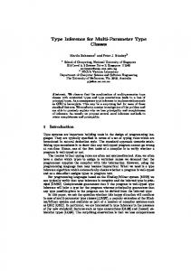
Classic W λ-Ranking let-Ranking

Pure W (Fig. 4) Wλ (Fig. 7) WL (Fig. 14)

Ref WV (Fig. 17) WλV (Fig. 19) WLV (Fig. 20)

Figure 1. Summary of Type Inference Abstract Machines cates its “position” in the type environment, where the type environment is viewed as ordered from outer to inner bindings. There are two main variants of this variable ranking approach. The one originally suggested by Damas [1] is based on depth of lambda bindings, and is used in SML/NJ. An equivalent alternative is based on depth of let bindings [13]. Although these implementation techniques have been used in compilers for a couple of decades, their formalization and proof of correctness has been largely neglected. Our goal is to begin to address that gap by proving that these ranked variable variants are equivalent to the original algorithm W. We start by considering type checkers for a pure form of microML (which we will call Pure ML), and then go on to introduce side-effects (ref) and the value restriction [18], calling this language variant Impure ML. Our approach is to formalize the various type inference algorithms that we will be studying using simple abstract machines such as those derived from small-step operational semantics for evaluation [2]. We then prove equivalences between these abstract machines, whose operation differs mainly at the point where polymorphic generalization occurs for let bindings. Since we have three variants of the type inference algorithm W (classic, lambda-ranked, and let-ranked) for two variants of the language (Pure and Impure ML), we have a total of six abstract machines, as shown in Fig. 1.

2.

An Abstract Machine for Classic Algorithm W

The abstract machines that we use here are simplified versions of the abstract machines used in an earlier paper [4], where we were viewing type checking and inference as a term-rewriting system that incrementally transformed expressions into their types. The abstract machines described below express type inference as a process of nonstandard evaluation of expressions, yielding their types. The language we will start with is the usual minimal ML, presented in Fig. 3. This language can easily be extended with constant expressions (e.g., numbers, booleans), and with additional basic type constructors (e.g., Int, Bool, List), and we will feel free to do so in examples. Later on we will introduce references, which will force us to complicate type inference by introducing the value restriction. Types (τ ∈ TYPE) are constructed over two forms of type variable. Polymorphic bound type variables (α, β, γ) will occur only in the bodies of polytypes (PTYPE) where they appear in the quantifier prefix – in other words, the types that occur during

W(Γ, x) W(Γ, λx.e) W(Γ, e e0 )

= = let in = let

in W(Γ, let x = e in e0 ) = let in

(id, I(Γ(x))) (θ, τ ) = W(Γ[x : ξ], e) ξ fresh (θ, θξ → τ ) (θ, τ ) = W(Γ, e) (θ0 , τ 0 ) = W(θΓ, e0 ) θ00 = U(θ0 τ, τ 0 → ξ) ξ fresh (θ00 θ0 θ, θ00 ξ) (θ, τ ) = W(Γ, e) (θ0 , τ 0 ) = W(θΓ[x : σ], e0 ) (θ0 θ, τ 0 ) σ = ∀α.{α/GΓ (τ )}τ

Figure 2. Algorithm W from Lee and Yi [5]

type inference will never contain free occurrences of such type variables. The other type variables (ξ, ζ, φ, ψ) are called unification variables, or univariables for short. They should be considered part of the internal machinery of type inference and should generally be eliminated from the final type produced.1 It should also be noted that although neither types nor polytypes (PTYPE) will contain free occurrences of polymorphic type variables, types and polytypes can both contain occurrences of univariables (which are necessarily free occurrences). We will use the term monotype for types τ ∈ TYPE to distinguish them from polytypes σ ∈ PTYPE, even though monotypes may contain free occurrences of univariables. For reference, Fig. 2 shows a standard version of algorithm W for Pure ML, following the modern presentation given in Lee and Yi [5]. This version differs from Milner’s original formulation [9] in that there are explicit generalization and generic instantiation steps that respectively introduce and eliminate polytypes. Note that W returns only monotypes τ as results, while both types and polytypes occur in type environments. We see that polytypes are created and then immediately entered into the type environment while processing let bindings. Sometimes, when no univariables are generalizable, these let-bound polytypes will be degenerate in the sense that the quantifier prefix is empty. New univariables are introduced at three points: (1) when entering a lambda abstraction, where we introduce a new univariable to represent the unknown type of the λ-bound variable, (2) when typing a variable, where we create a generic instance of the polytype bound to the variable in the type environment, and (3) in the application case, where we introduce a fresh univariable to represent the return type before unifying. Conversely, univariables can be eliminated (1) by being instantiated (i.e. replaced by substitution), or (2) by being generalized at a let binding. Using standard methods [14], we can transform the classic algorithm of Fig. 2 into the abstract machine in Fig. 4. The abstract machine states consist of three components, or registers. The control, the first register, can be either the next (sub)expression we are type checking or a monotype produced by completing the typing of a subexpression. The type environment, the second register, maps program variables to either monotypes (for λ bindings) or polytypes (for let bindings). The type environment context is an ordered sequence of λ and let-bindings that map expression variables to their types, with the outermost bindings first, so that the λ and let-nesting is reflected in its binding order. The distinction between let and lambda bindings is indicated 1 A top level expression like λx.x will be assigned a type ξ → ξ containing a free univariable. We can eliminate this univariable by supplying an implicit top level let declaration context for the expression, typing it as let it = λx.x where the scope is the “rest of the program”. Then the univariable can be eliminated by generalization. If the value restriction applies this will not always work (e.g., ref nil), and we may have to eliminate the univariables by dummy instantiation with arbitrary ground types, as is done in the SML/NJ type checker.

e τ σ

::= ::= ::=

x | λx.e | e1 e2 | let x = e1 in e2 α|ξ|τ →τ ∀α.τ

EXP TYPE PTYPE

Figure 3. Pure ML mini-language by whether the type in the binding is a polytype (possibly degenerate) introduced by a let, or a monotype, introduced by a lambda. The stack, the final register, represents a typing continuation that keeps track of what still needs to be done to complete the type checking. λ and let stack frames tell the machine when to pop off associated λ- and let-bindings from the type environment (i.e., when the type checker is leaving the scope of the λ or let body). ( e) and (τ ) frames save relevant context information when type checking the operator and operands of applications. Finally, let x in e frames tell the machine to generalize the control type, which must be the type of the definien, and to add the resulting polytype to the type environment when type checking the body e. As in the original algorithm W, polytypes are only introduced by [let-body], which puts them in the environment. The [var] rule looks up a variable in the type environment and immediately applies I to generically instantiate the result, eliminating the polytype and (possibly) introducing fresh univariables. Consequently, polytypes only exist in the typing context and are never found in the control. The [λ-in] rule pushes a new λ-binding onto the type environment, with a fresh univariable as the type of the bound variable. Simultaneously, a λ frame is pushed onto the stack as a reminder to pop off the associated λ binding when we have finished type checking the body. The [λ-out] rule pops off the λ-binding and constructs the function type to complete the typing of an abstraction. The [let-out] rule plays an analogous role for let expressions, popping the let-binding from the typing context and returning the body type. The remaining rules essentially serve as search rules. The [app-out] rule sets up the function-argument agreement constraint, using a fresh univariable, and solves it by unification (U defined in Fig. 5). In the process, the unification may eliminate some univariables. Unification fails (in a stuck state) if the function and argument cannot be made to agree, in which case a type error is signaled. It is straightforward to show that the Algorithm W abstract machine of Fig. 4 is equivalent to the classical algorithm of Fig. 2, in the sense that for any closed expression e, W(e, ∅) = (τ, θ) ⇔ (e, ∅, •) 7→ (τ, ∅, •)

(1)

and we therefore take the abstract machine as our reference implementation from here on.

3.

Depth Ranking Techniques

Let us make some some key observations about the effect of substitutions on the occurrence of univariables in type environments, which is the critical factor in deciding whether a univariable can be generalized. First note that for any ξ ∈ ftv(Γ) we can define the the rank of ξ relative to the environment Γ as the index (counting from 1) of the first (i.e., outermost) binding in Γ containing an occurrence of ξ. We will denote this rank by R(ξ, Γ). If ξ 6∈ ftv(Γ), we define R(ξ, Γ) = ∞. So at a let binding, a univariable is generalizable if and only if its rank relative to the current type environment is infinite: ξ ∈ GΓ (τ ) ⇔ ξ ∈ ftv(τ ) and R(ξ, Γ) = ∞ Another useful observation is that at a let binding, if we generalize relative to the current environment Γ to get a polytype σ and add the polytype binding [x : σ] to Γ, then any univariable ξ ∈ ftv(σ)

Γ f k c s

::= ::= ::= ::= ::=

∅ | Γ[x : τ ] | Γ[x : σ] λ | ( e) | (τ ) | let x in e | let • | f :: k e|τ (c, Γ, k)

Tyenv Frames Stack Control States

Initial States s0 = (e, ∅, •) (x, Γ, k) 7→ (I(Γ(x)), Γ, k) (λx.e, Γ, k) 7→ (e, Γ[x : ξ], λ :: k) ξ fresh (τ, Γ[x : τ 0 ], λ :: k) 7→ (τ 0 → τ, Γ, k) (e1 e2 , Γ, k) 7→ (e1 , Γ, ( e2 ) :: k) (τ, Γ, ( e2 ) :: k) 7→ (e2 , Γ, (τ ) :: k) (τ, Γ, (τ 0 ) :: k) 7→ (θξ, θΓ, θk) where θ = U(τ 0 , τ → ξ), ξ fresh (let x = e1 in e2 , Γ, k) 7→ (e1 , Γ, let x in e2 :: k) (τ, Γ, let x in e2 :: k) 7→ (e2 , Γ[x : σ], let :: k) where σ = ∀α.{α/GΓ (τ )}τ, α fresh (τ, Γ[x : σ], let :: k) 7→ (τ, Γ, k) GΓ (τ ) = ftv(τ ) − ftv(Γ) I(∀α.τ ) = {ξ/α}τ where ξ is fresh I(τ ) = τ

[var] [λ-in] [λ-out] [app-l] [app-r] [app-out] [let-def] [let-body] [let-out]

a univariable to an earlier binding and thus make it “less generalizable”. As we have defined it, computing the rank of a univariable relative to an environment is no less expensive than computing whether it occurs in the environment. But the main idea of the ranked variable algorithms we will present below is that we can avoid scanning the environment by making the rank an attribute of the univariable and managing that attribute incrementally so that it is always equal to the intrinsic rank defined above, relative to the current environment in the machine state. Since in the W machine for Pure ML, only the λ bindings count, our first version of univariable ranking will assign ranks based on the depth of λ nesting (i.e. counting only λ bindings). We will then look at a variant for Pure ML that counts only let definien marks (which demarcate the scopes of nested let definiens). When we introduce references and the consequent requirement for the value restriction, things become more complicated, because the invariant that univariables first occur in λ bindings will no longer be the case, and non-value let bindings will act like λ bindings.

Generalization

4. λ-Depth Ranking

Generic Instantiation

In Figs. 6 and 7, we modify the Pure ML inference machine by adding ranks to the univariables. The rank associated with a univariable is either a natural number or ∞, and if a univariable occurs in the current type environment its rank is meant to correspond to the index of the earliest λ-binding in the environment in which it occurs. A rank greater than the number of λ bindings in the current environment will indicate that the univariable is generalizable, i.e. its intrinsic rank is ∞. For convenience, we add a new register to the machine states containing the current λ nesting depth d. This register starts at 0 and counts how many λ-abstractions we have passed through to reach to the current control. Its value will always be equal to both the number of λ-bindings in the current environment and the number of λ frames in the context stack. The W machine rules are easily adapted to incorporate λ-depth ranking, and we will call this new machine Wλ . The new [λ-in] rule increments the depth, introduces a fresh univariable whose initial rank is the new λ nesting depth, and pushes a new λ binding onto the environment. The [λ-out] rule now also decrements the depth. We can categorize bindings in type environments according to whether they are introduced by the [let-body] rule, in which case the variable is bound to a polytype σ, or by the [λ-in] rule, in which case the variable is bound to a monotype τ (and this distinction is preserved under substitution). This distinction on bindings is expressed in the definition of environments in Fig. 7. As noted in the previous section, if a univariable occurs in an environment, the first binding it occurs in will always be a λ-binding, and let-bindings play a secondary role. So we can modify the notion of the occurrence index of a univariable ξ in an environment Γ, which we called the intrinsic rank R(ξ, Γ), by counting only λbindings from left to right when we calculate this index. The univariable ranks in the Wλ machine are assigned and managed so that they always correspond to the intrinsic rank determined by the location of the univariable in the current environment (if any). Note that because applying unification substitutions in [appout] can “promote” univariables to earlier λ-bindings, the first λbinding containing a univariable may not correspond to the program point where it was introduced. A substitution that promotes a univariable to an earlier binding must compensate for the change in the intrinsic rank of the univariable by adjusting the explicit rank of the univariable to reflect its new earliest occurrence in the environment. The L limit substitution defined in Fig. 8 performs this necessary adjustment to univariable ranks. When a unification substitu-

Figure 4. Algorithm W Abstract Machine U(τ, τ ) = ε

U(τ, ξ) = U(ξ, τ ) where τ is not a univariable U(ξ, τ ) = {τ /ξ} if ξ ∈ / ftv(τ ) U(τ1 → τ2 , τ3 → τ4 ) = U(θ(τ2 ), θ(τ4 )) ◦ θ where θ = U(τ1 , τ3 )

Figure 5. Unification already appeared in Γ, i.e., ξ ∈ ftv(Γ). This is because if ξ did not appear in Γ, it would have been generalized and replaced by a polymorphic bound type variable. Thus, at the point where it is added, a let binding introduces no new univariables into the environment. It also means that the first occurrence of a univariable in the environment is always at a λ binding. These properties are obviously preserved if a type substitution is applied to a type environment. So we have the invariant (for Pure ML): 1. The first occurrence of a univariable in an environment is always at a λ binding. Now let us consider the effect of a substitution on the rank of a univariable in an environment. Consider a univariable ξ, an environment Γ, and a type substitution θ. What is the relation between R(ξ, Γ) and R(ξ, θΓ)? If ξ ∈ dom(θ), then ξ is eliminated by θ (remember that all our substitutions are idempotent because of the occurrence check), so R(ξ, θΓ) = ∞. But in this case, since θ is applied uniformly to all components of the abstract machine, ξ is eliminated everywhere, and its rank is no longer relevant since we will never ask whether ξ can be generalized. Next assume that ξ 6∈ dom(θ). Then applying θ to Γ will not remove any occurrences of ξ, so the rank of ξ in Γ will not increase, but it could decrease if ξ occurs in the range of θ and new occurrences of ξ are added in θ(Γ) (including the case where ξ 6∈ ftv(Γ) but ξ ∈ ftv(θ(Γ)). Hence R(ξ, θ(Γ)) ≤ R(ξ, Γ) if ξ 6∈ dom(θ) Thus, except for the case where a univariable is eliminated by a substitution, a substitution can only decrease the rank of a univariable or leave it the same. This means that a substitution may “promote”

e τ d σ

x | λx.e | e1 e2 | let x = e1 in e2 ξd | τ → τ | α 0 | 1 | 2 | ... | ∞ ∀α.τ

::= ::= ::= ::=

EXP TYPE Ranks PTYPE

[x : . . .ξ 1 . . .]λ [. . .]let

Figure 6. λ-Ranking Language

λ-binding Index

Γ ::= ∅ | Γ[x : τ ] | Γ[x : σ] f ::= λ | ( e) | (τ ) | let x in e | let k ::= • | f :: k c ::= e | τ s ::= (c, Γ, d, k) Initial State s0 = (e, ∅, 0, •)

Tyenv Frames Stack Control States

(x, Γ, d, k) → 7 λ (I(Γ(x)), Γ, d, k) (λx.e, Γ, d, k) → 7 λ (e, Γ[x : ξ d+1 ], d + 1 λ :: k) (τ, Γ[x : τ 0 ], d, λ :: k) 7→λ (τ 0 → τ, Γ, d − 1, k) (e1 e2 , Γ, d, k) 7→λ (e1 , Γ, d, ( e2 ) :: k) (τ, Γ, d, ( e2 ) :: k) 7→λ (e2 , Γ, d, (τ ) :: k) (τ, Γ, d, (τ 0 ) :: k) 7→λ (θξ ∞ , θΓ, d, θk) θ = U(τ 0 , τ → ξ ∞ ) (let x = e1 in e2 , Γ, d, k) 7→λ (e1 , Γ, d, let x in e2 :: k) (τ, Γ, d, let x in e2 :: k) 7→λ (e2 , Γ[x : σ], d, let :: k) σ = ∀α.{α/Gd (τ )}τ where α is fresh (τ, Γ[x : σ], d, let :: k) 7→λ (τ, Γ, d, k) Gd (τ ) I(∀α.τ ) I(τ )

= = =

{ξ m ∈ ftv(τ ) | m > d} {ξ ∞ /α}τ τ

[λ-out] [app-l] [app-r] [app-out] [let-def] [let-body]

[y : . . .φ2 . . .]λ 2

U(ξ 1 , . . . φ2 . . .)

(a) If ξ (a contextual variable) instantiates to y’s type, then φ (a local variable) propagates into x’s λ-binding.

[x : . . .φ2 . . .]λ [. . .]let λ-binding Index

[var] [λ-in]

1

[y : . . .φ2 . . .]λ

1

2

(b) The rank of φ must now be limited to that of ξ because the first occurrence of φ has shifted left, thus making it contextual.

[x : . . .φ1 . . .]λ [. . .]let λ-binding Index

[y : . . .φ1 . . .]λ

1

2

(c) After Applying the Limit Substitution

Figure 9. Limit Substitution (L) Example: Subscripts on bindings indicate the kind of binding.

[let-out]

Generalizable Generic Instantiation

Figure 7. Algorithm W Machine extended with λ-depth Ranking (Wλ ) U (τ, ξ m ) = U (ξ m , τ ) where τ is not a univariable U(ξ m , τ ) = Lm (τ ) ◦ {τ /ξ m } if ξ m ∈ / ftv(τ ) U(τ1 → τ2 , τ3 → τ4 ) = U(θ(τ2 ), θ(τ4 )) ◦ θ where θ = U(τ1 , τ3 ) Ld (τ ) = {ξ d /ξ m | ξ m ∈ ftv(τ ) ∧ m > d} U(τ, τ ) = ε

[x : . . .ξ 1 . . .]λ [. . .]let λ-binding Index

1

[y : . . .φ2 . . .]λ

U(φ2 , . . . ξ 1 . . .)

2

(a) If φ instantiates to x’s type, then ξ propagates into y’s λ-binding.

[x : . . .ξ 1 . . .]λ [. . .]let λ-binding Index

[y : . . .ξ 1 . . .]λ

1

2

(b) ξ’s rank is fine because its first occurrence has not shifted. It remains contextual.

Figure 10. Example of when the limit substitution is unnecessary

Figure 8. Unification with λ-rank Maintenance tion maps a univariable ξ to a type τ , univariables occurring in τ may be introduced to λ-bindings to the left of their original first occurrences, if ξ occurs earlier in the environment. Thus, if the first occurrence of ξ was to the left of the first occurrence of some univariable φ ∈ ftv(τ ), then after unification, the first occurrence of φ is now where the first occurrence of ξ was before as shown in Fig. 9. If the first occurrence of ξ was to the right of the first occurrence of φ, then the first occurrence of φ does not move after unification as shown in Fig. 10. As a simple example of this issue, consider the expression λx.let y = λz.xz in . . .. The λ bindings for x and z produce an environment Γ = [x : ξx1 ][z : ξz2 ] for the typing of the application xz. The typing of this application involves a unification producing the substitution θ = ξx1 7→ (ξz2 → ξr∞ ). But if θ is applied to the typing environment it would produce Γ0 = [x : ξz2 → ξr∞ ][z : ξz2 ] in which the ranks of the univariables in the x binding no longer correspond to its index in the environment, which is 1. So an additional rank limiting substitution is required to adjust the ranks of ξz and ξr downward: (ξz2 7→ ξz1 , ξr∞ 7→ ξr1 ). When this is applied we get a properly ranked environment Γ0 = [x : ξz1 → ξr1 ][z : ξz1 ]. Now the adjusted rank of ξz1 will prevent the type of y, namely ξz1 → ξz1 from being generalized at the let binding.

Definition 1 (Valid Machine States (VMS)) A machine state (c, Γ, d, k) is valid if it is reachable from some valid initial machine state (e, ∅, 0, •) (i.e., (e, ∅, 0, •) 7→∗ (c, Γ, d, k) where 7→ is the machine transition relation). From this point on, a metavariable with a tilde (˜) on top denotes the corresponding instance of that construct where the ranks of any univariables that occur are erased or ignored. Definition 2 e |Γ| = the length of Γ, and similarly for |Γ|. Definition 3 e D(Γ) = # λ bindings in Γ, and similarly for D(Γ). Definition 4 eλ . Γλ denotes the list of λ-bindings in Γ, and similarly for Γ

Definition 5 (Intrinsic Univariable Rank) e ∅) R(ξ, e e R(ξ, Γ[x : τe]) e Γ[x e :σ R(ξ, e])

= = = =

Proof: By induction on the length of Γ and Lemma 3

We also make a simple observation about substitutions and environments that simplifies the proofs in Lemma 5.

∞ e Γ), e D(Γ) e + 1) if ξ ∈ ftv(e min(R(ξ, τ) ∞ otherwise e Γ) e R(ξ,

Lemma 5 (Substitution Range Preservation) If τ ∈ rng Γ, then στ ∈ rng σΓ.

This computes the index of the first λ-binding containing an occurrence of a univariable, ignoring let-bindings. If a univariable is not in the environment, it is assigned the intrinsic rank ∞, which ensures that such a univariable should be generalized because it is always greater than any let expression’s finite λ-depth. Definition 6 e Er (Γ)) R(ξ m , Γ) = R(ξ, where Er erases the ranks of univariables in Γ. By definition, type environments can be extended with more bindings. We formally define the notion of extension: Definition 7 e 0 is an extension of Γ e if and only if there exists Γ e 00 such that Γ e0 Γ e and Γ e 00 (in that order). is the concatenation of Γ Notice that if a type variable occurs in a type environment, then extension of that type environment does not change that type variable’s leftmost occurrence: e Invariant Under Γ e Extension) Lemma 1 (R e and Γ e 0 is an extension of Γ, e then R(ξ, e Γ e0 ) = If ξ ∈ ftv(Γ) e Γ). e R(ξ, e Proof: By induction on the length of Γ



e computes the first occurrence index for a univariable Because R in an environment, if a univariable does occur in the environment e will return the same index for any extension of that environment. R e counts the number of λ-bindings up to a By definition, R univariable’s first occurrence. Naturally, this number cannot exe We observe this fact in ceed the total number of λ-bindings on Γ. Lemma 2. Lemma 2 e λ ), then R(ξ, e Γ) e ≤ D(Γ). e If ξ ∈ ftv(Γ e Proof: By induction on the length of Γ



We determined by construction that the rank of a univariable that does not occur in the environment is ∞. This is formally stated in Lemma 3. Lemma 3 e λ ) then R(ξ, e Γ) e = ∞. If ξ ∈ / ftv(Γ e Proof: By induction on the structure of Γ





To formalize the notion of first occurrence of a univariable, we appeal to Lemma 4. Lemma 4 If ξ m occurs in the n-th λ-binding in Γ (counting from the left) and ξ m occurs in no λ-binding to the left of that n-th λ-binding, then R(ξ m , Γ) = n.

Proof: This follows from definition of type variable substitution on type environments.  Definition 8 (Properties for Wλ ) The following are invariant properties on any valid Wλ machine state s = (c, Γ, d, k): Prop1 ∀ξ m ∈ ftv(Γ), R(ξ m , Γ) = m Prop2 ∀ξ m ∈ ftv(c) such that m ≤ D(Γ), then ξ m ∈ ftv(Γ) Prop3 D(Γ) = # of λs on k Prop4 ∀ξ m ∈ ftv(k) such that m ≤ r where r is the number of λ frames below the frame with the occurrence of ξ m in the stack k, ξ m ∈ ftv(Γ) Prop1 asserts that a univariable’s rank corresponds to the index of the λ-binding containing the first occurrence of that univariable in the environment. This is a precursor to Corollary 1 below that provides a notion of completeness for the λ-ranking scheme. All univariables in the environment must be given a low rank. Prop2 says that all the “contextual” univariables occurring in the control are bound in the environment. Contextual refers to having a rank no greater than D(Γ). This specifically excludes univariables that would run off the end of the environment at the current scope because their ranks are too great, including univariables with rank ∞. Prop2 asserts that all low ranked univariables must be in the environment. Therefore it provides a notion of the soundness of the ranking scheme. Prop3 tells us that the number of λ-bindings in the environment corresponds to the λ-nesting depth. This simple observation is necessary for establishing Prop1 when only λ-depth information is available. Prop4 is a rather subtle property. It ensures that the a modified version of Prop2 holds for those univariables occurring on the stack in (τ ) frames. Because the type τ of the operator is in a sense “parallel” to the current operand expression that the machine is working on, it may contain some seemingly low ranked univariables (rank < current λ-depth) that are not in the current environment for the operand. These univariables are not truly low ranked because at the point when (τ ) was pushed onto the stack, τ was in the control, so by Prop2 any univariables not in the environment at that point had rank higher than the D(Γ0 ), where Γ0 was the then-current environment. But D(Γ0 ) was also equal to the number of λ frames on the stack before the (τ ) frame was pushed. Once the machine pops all the frames sitting on top of the (τ ) frame, the environment will once again have its original λdepth. For example, in (λx.x)(λy.λz.z), before the machine reaches the body of λz.z, λx.x is given the type ξ 1 → ξ 1 . When typing the body of λz.z, the λ-depth is 2. It seems that ξ 1 has a low rank. However, at the point we were just finished with λx.x and when we pop out of the operand, the λ-depth is 0. Therefore ξ 1 is actually a high ranked univariable that we do not expect to find in the environment when we get back to it. We proceed by first showing that these properties are invariant under the unification that results from [app-out].

Lemma 6 (Invariants under unification) For all Γ, if the properties from def. 8 hold for s = (τ, Γ, d, (τ 0 ) :: k) ∈ VMS and θ = U(τ 0 , τ → ψ ∞ ) (where ψ ∞ is fresh), then the properties must also hold for s0 = (θψ ∞ , θΓ, d, θk).

The rest of the cases are fairly straightforward case analyses assuming that the properties holds before each transition rule. 

Proof (sketch): This proof is by induction on sizes of τ 0 and the other type argument of U . The instantiation case is the interesting part of this proof. In that case, by definition of unification, θ = U(φn , τ ) = Ln (τ ) ◦ {τ /φn }. The interesting cases for Prop1 (s0 ) are illustrated in Figs. 10 and 9. In the first case, assume ξ m ∈ ftv(θΓ) was not limited, hence it must have a rank that is lower or equal to n. Because φn was substituted away by θ, it must occur in Γ. By, Lemma 2, n ≤ D(Γ). Thus, m ≤ D(Γ). By Prop2 (s), ξ m must occur in Γ. By Prop1 (s), R(ξ m , Γ) = m. In the case where ξ m was limited, the first occurrence of ξ m shifted left to the former first occurrence of φn . Thus, it should also receive rank n. Lem. 4 helps establish this. For Prop2 (s0 ), the unlimited case is simple. The case where ξ m was limited is somewhat tricky. If the univariable to be instantiated φn has a rank n > D(θΓ), the case is vacuous, so assume that m ≤ D(θΓ). Note that by the definition of L, m = n. We first have to show that φn must be in Γ. φn can come from τ , τ 0 , or ψ ∞ . The ψ ∞ case is vacuous because ∞ > D(Γ). The τ case is handled by Prop2 (s). The τ 0 case takes a little more work because Prop2 (s) did not say anything about τ 0 . This is the reason why we need Prop4 . Prop4 (s) gives us what we need. Assuming that φn ∈ ftv(Γ), it is straightforward to show that ξ m ∈ ftv(Γ) with the help of Lemma 5. Prop3 (s0 ) is easily to establish because substitution does not change the length of Γ or k. Prop4 is also relatively straightforward. 

Corollary 1 (Ranking is Complete) For all Γ from s = (c, Γ, d, k) ∈ VMS ξ m ∈ ftv(Γ) ⇒ m ≤ D(Γ)

The properties trivially hold for the initial states. Now we proceed to show that the properties are indeed invariant under all machine transition rules. This would establish that the properties are invariants over all valid machine states. Lemma 7 (Properties invariant over all machine transitions) If the props. in def. 8 hold for s ∈ VMS and s 7→λ s0 , then they must hold for s0 . Proof (sketch): We need Prop3 to push through Prop1 ’s [λ-in] case, thus showing that the ranks do measure λ nesting depth. This fact combined with Lemma 3 establish that the ranks correspond to the λ-binding index of the first occurrence (actually the only occurrence) of the fresh univariable representing this λ’s parameter type in the environment. For the [λ-out], [let-body], and [let-out] cases, we use Lemma 1 to show Prop1 . For [app-r], Prop4 (s0 ) simply inherits the property from Prop2 (s) because τ merely shifted from the control to the top of the stack. Prop1 and Prop2 for the [app-out] case follow from Lemma 6. For Prop1 in the [let-body] case, we use Prop2 ’s prop. that we assume holds before transitioning by [let-body] to show that any univariable ξ in ftv(Γ[x : σ]) must also occur in ftv(Γ). That is to say, first occurrences of univariables in environments are never in let-bindings. We can then conclude by assumption and Lemma 1 that R(ξ m , Γ[x : σ]) = m. For Prop2 , we note that ξ m ∈ ftv(τ 0 → τ ) in [λ-out] cannot have a first occurrence in the last binding in Γ[x : τ 0 ] because by assumption, m ≤ D(Γ). If this were not the case, then we would be seeing unbound yet non-generic univariables after [λout] transitions.

From Prop1 , we can easily obtain a completeness corollary.

Proof (sketch): By Prop1 from Lemma 7, R(ξ m , Γ) = m. Since D(Γ) = |Γλ |, m ≤ D(Γ) by definition of R and Lemma 2.  We can put together Corollary 1 and Prop2 to establish that the ranking corresponds to searching through the environment for all valid machine states. Lemma 8 For any (τ, Γ, d, k) ∈ VMS and ∀ξ m ∈ ftv(Γ), m ≤ d iff ξ m ∈ ftv(Γ). Proof: ⇒ : This direction follows from Prop2 of Lemma 7. ⇐ : This direction follows from Corollary 1. m ≤ D(Γ) = d  The generalizability criteria are equivalent. Consequently, we always generalize the same set of univariables using the classical and λ-ranking algorithms. Lemma 9 (Equivalence of Generalizability Criteria) If (τ, Γ, d, let x =  in e :: k) 7→ (e, Γ[x : σ], d, let :: k) where σ = ∀α.{α/Gd (Γ)}τ , then Gd (Γ) = GΓ (Γ). Proof: This proof falls out from the definitions of Gd and GΓ , and Lemma 8.  Finally, we put everything together. The classical algorithm W and the λ-ranking algorithms are equivalent. Theorem 1 (Equivalence to Classical Algorithm W) (e, ∅, 0, •) 7→∗ (τ, ∅, 0, •) iff (e, ∅, •) 7→∗ (τ, ∅, •). Proof: We only inspect the depth register in [let-body]. In all other cases, the λ-ranking and classical machines are identical. The depth register is only along for the ride. Because of Lemma 9, the [let-body] behaviors are also identical. 

5.

Let-Depth Ranking

The let-depth ranking scheme is similar to the λ-depth ranking except for a few significant adjustments. We can reuse the language and the same notation for ranks. The main observation that the letdepth ranking relies on is that the locality of univariables at different λ-depths is the same as long as we are in the same let definien’s scope. In contrast, λ-ranks distinguish among λ’s at different λnestings even though they may all be in the same let definien scope. We have to be careful, though, because a let expression only extended the type environment when the type checker reaches the body. At that point, generalization of the definien type would have already occurred. So we cannot use let-bindings to derive a ranking for determining generalization. We have to determine a rank before generalization occurs. So, we turn to another implicit structure of the environment, the partitioning of bindings into contiguous

λx.let a = λy1 .λy2 .let b =let c = • in . . . in . . . in . . .

Lambda Rank

λ

λ 1

Environment at •: [x : ξ 0 ][y1 : ζ 1 ][y2 : φ1 ]

Figure 11. When we reach •, we pass into three let definiens but added no let-bindings to the environment. The type of x is less generalizable than that of the y’s. The type of the y’s should be generalizable at the same point.

Let Rank

0

let d

let b

λ

d

let

λ

2

let a = λx.let b = . . . in let c = . . . in (λy.y)• in . . .

λ

λ 2

λ 2

λ 1

0

let

Figure 12. When we reach •, we are in no let definiens but added two let-bindings to the environment. The types of x and y are both generalizable at the let a.

λs.let x = λt.. . . in let y = λu. . . .

let 1

Environment at •: [x : ξ 1 ][b : σb ][c : σc ][y : ζ 1 ]

blocks according to the definien scope. We can extend the machine introduced in Wλ to make this let definien partitioning manifest. We cannot naively replace λ’s with let’s in the development from the previous section to get a working let-ranking scheme. In particular, λ’s were simple. We only traverse a λ-abstraction in one pass. First, we extend the environment with the bound λvariable. Then we traverse the body of the λ using this extended environment. Once we are done, we pop out of the λ never to revisit it. In contrast, for let’s, we have to first traverse the definien without extending the environment, pop out of the definien, extend the environment with the generalized definien type, and only then traverse the body of the let with this extended environment. We have to increment the depth when we pass into a definien, as for instance in the expression λx.let y = x in . . ., where we need to prevent the type of x from being generalized where y is bound. On the other hand, the body should have the depth that held before we entered into the definien. This permits the type of λy.y to generalize in let x = let . . . in λy.y in . . .. The complication is that there is no simple connection between the number of letbindings in the environment and the number of let definiens we have passed into (but have not finished typing). Figs. 11 and 12 give examples of this problem. In the environments for the two examples, we label the univariables with the let definien depth at the point of introduction. Although in Fig. 11 ξ has a lower let definien depth than ζ and φ, there is nothing in the environment to demarcate the two groups of bindings. In Fig.12, ξ and ζ have the same depth and yet they are separated by two let-bindings. To overcome this problem, we rank by the number of let definien letd markers in an environment instead of λ-bindings. We want to identify contiguous blocks of λ-bindings in the environment that are within the same let definien scope. Thus, every time we pass into a let definien, we mark the (rightmost) end of the environment with a letd marker. This marker tells us that any λ to left of the marker will be less generalizable than any λ that will be to the right. We extend the definition of Γ with these letd marks in Fig. 14. The letd marked versions of the environments in Figs. 11 and 12 would be [x : ξ 0 ][letd][y1 : ζ 1 ][y2 : φ1 ][letd][letd] and [letd][x : ξ 1 ][b : σb ][c : σc ][y : ζ 1 ] respectively. Fig. 13 shows both the λ and let ranking of the following program:

b

let

λ

λ 3

1

Figure 13. Comparison of λ and let ranks in expression structure in λv.

let z = λw. . . . in . . .

The left branch of each let node represents its definien (d) and the right branch its body (b). The dashed lines indicate where we increment the rank. In this example, there are no let definiens nested in another let definien, hence generalizability at a let definien is determined solely by whether a univariable is local to that let definien or outside of any let definien. Univariables at that let definien could not have been introduced in another let definien because they would have already been generalized at that earlier (to the left) let definien or we would have not reached that let definien yet. Notice that the λ ranking method increments the rank much more frequently. In fact, the distinction between ranks on the right spine of the program does not make a difference with respect to generalizability. For example, the types of s and v are in the same scope of generalization (i.e., they are both outside of all let definiens). The let ranking method only increments the rank at the let definiens where the rank distinction may make a difference with respect to generalizability. Definition 9 (Let Depth) e = # of letd markers in Γ e Dlet (Γ)

Definition 10 (Univariable Let-Rank) e let (ξ, ∅) R e e : τe]) Rlet (ξ, Γ[x

= =

e let (ξ m , Γ[x e :σ R e])

=

∞ e let (ξ, Γ), e m) min(R e if ξ ∈ ftv(e where m = Dlet (Γ) τ ), otherwise m = ∞ e let (ξ m , Γ) e R

Definition 11 e let (ξ, Er (Γ)) Rlet (ξ m , Γ) = R

Γ ::= Γ[letd] | . . . s = (c, Γ, d, k) Initial Machine State s0 = (e, ∅, 0, •)

Γ with let definien marks states

(x, Γ, d, k) → 7 L (I(Γ(x)), Γ, d, k) (λx.e, Γ, d, k) → 7 L (e, Γ[x : ξ d ], d λ :: k) (τ, Γ[x : τ 0 ], d, λ :: k) 7→L (τ 0 → τ, Γ, d, k) (e1 e2 , Γ, d, k) 7→L (e1 , Γ, d, ( e2 ) :: k) (τ, Γ, d, ( e2 ) :: k) 7→L (e2 , Γ, d, (τ ) :: k) (τ, Γ, d, (τ 0 ) :: k) 7→L (θξ, θΓ, d, θk) θ = U(τ 0 , τ → ξ ∞ ) (let x = e1 in e2 ,Γ, d, k) 7→L (e1 , Γ[letd], d + 1, let x in e2 :: k) (τ, Γ[letd], d, let x in e2 :: k)

[wl-var] [wl-λ-in] [wl-λ-out] [wl-app-l] [wl-app-r] [wl-app-out] [wl-let-def]

[wl-let-body] 7→L (e2 , Γ[x : σ], d − 1, let :: k) let σ = ∀α.{α/Gd (τ )}τ, α is fresh (τ, Γ[x : σ], d, let :: k) 7→L (τ, Γ, d, k) [wl-let-out] Gdlet (τ ) = {ξ m ∈ ftv(τ ) | m ≥ d} Generic instantiation I, language, stack register k, and frames f remain the same as in the Wλ machine in Fig. 7.

As in Wλ , we generalize univariables of rank greater than the depth at the point of generalization where we have popped out of the definien (and thus decremented the depth). Any univariables that we introduced inside the scope of the definien must have rank greater than or equal to the index of the letd mark we just popped off. R´emy’s let-ranking scheme generalizes only those univariables that have rank exactly equal to the current depth [13]. This is due to a difference between how his and our systems rank generic univariables. His system ranks generic univariables with the current depth instead of ∞. e hold for R e let . Many of the lemmas about the construction of R Lemma 10 (Rank is ∞ if not in Γ) e λ ), then R e let (ξ, Γ) e = ∞. If ξ ∈ / ftv(Γ e Proof (sketch): By straightforward induction on Γ



Lemma 11 If ξ m occurs in a λ-binding in Γ that is left bounded by the nth letd mark and ξ m occurs in no λ-binding to the left of that letd, then Rlet (ξ m , Γ) = n.

Figure 14. Algorithm W Machine with let-Ranking (WL ) Proof (sketch): By induction on Γ and lem. 10 The univariable rank no longer indicates the exact λ-binding that has the first occurrence in the environment. Instead, the rank is the index of the nearest letd marker to the left of the λ-binding with the first occurrence. We can call this the left bounding letd marker for the first occurrence. Multiple, distinct univariables can share the same left bounding letd mark. These univariables have the same generalizability. As before, generic univariables are rank ∞. Univariables that are bound outside of any let definiens are rank 0. If the environment was [x : ξ][letd1 ][y1 : φ1 ][y2 φ2 ][letd2 ][z : ζ], then ξ, φ1 , φ2 , and ζ would be ranked 0, 1, 1, and 2 respectively. The left bounding letd’s for the φ’s and ζ are letd1 and letd2 ree R e let still igspectively. Also, similar to the Wλ rank function R, nores let-bindings when computing the rank. As we have shown before, let-bindings have nothing to do with rank and generalizability. Fig. 14 gives an abstract machine for a type inference algorithm that uses let-ranking. The [wl-λ-in] and [wl-λ-out] rules do change the depth counter. This is now the responsibility of the [wl-let-def] and [wl-let-body] rules that introduce and eliminate the let x in e definien binder frame on the stack respectively. We can reuse the definition of unification from the λ-ranking system because it turns out that we can use L limit substitution with no changes except for using the let-ranks in place of the λranks. Since instantiation during unification still shifts around the first occurrence in exactly the same way it did before, the limit substitution is still necessary in those cases where a univariable of low rank is instantiated with a type with univariables of high rank. Because it is easier for univariables to share the same let-rank than to share λ-ranks, we do not expect the limit substitution to apply as often as it did with the λ-ranking. The [wl-let-body] rule decrements the let-depth, pops the let x in e2 frame off the stack and the letd frame off the environment, and pushes a let onto the stack. When type checking the body of a let-expression, that let will introduce no additional polymorphism because it already generalized the types for the definien. Thus, the [wl-let-body] pops out from the definien’s scope of generalization. This is why [wl-let-body] decrements the let depth. In contrast to Wλ , the type environment is augmented but the depth is decremented. The let frame on the stack is a reminder to pop off this new let-binding on the environment.



The properties also carry over with minimal changes. Definition 12 (Properties on WL Machine States) The following are the properties on valid WL machine states (c, Γ, d, k): Prop1 For all ξ m ∈ ftv(Γ). R(ξ m , Γ) = m Prop2 For all ξ m ∈ ftv(c) ∪ ftv(k) such that m ≤ Dlet (Γ), ξ m ∈ ftv(Γ) Prop3 Dlet (Γ) = # of let x in e’s (let definien frames) on k Prop4 For all ξ m ∈ ftv(k) such that m ≤ r where r is the number of let x in e frames up to the frame with the occurrence of ξ m on the stack k, ξ m ∈ ftv(Γ).

Lemma 12 (Properties Invariant Under Unification) If the def. 12 hold for machine state valid WL machine state (τ, Γ, d, k) and θ = U (τ 0 , τ → ζ ∞ ) and τ 0 occurs in k and ζ is fresh, then those properties hold for (θc, Γ, d, k). Proof (sketch): This proof is very similar to that of Lemma 6. As the example in Fig. 15 shows, the limited univariable case also plays out as it did for Wλ . The difference is that we look for left bounding letd marks for λ-bindings with first occurrences instead of the λ-bindings themselves.  Again, the properties hold trivially for the initial WL states, hence we only have to show that they hold under all the transition rules. Lemma 13 (Properties Are Invariant For WL ) For all valid WL machine states s, if the def. 12 properties hold for s and s 7→L s0 , then the properties must hold for s0 . Proof (sketch): This proof is similar to lem. 7. Lemma 12 provides the proof for the [wl-app-out] case. The two proofs differ in that some of the work for the [λ-out] case is shifted to the [wllet-body] since now it does the rank decrementing. The intuition is that the environment and the stack are synchronized. Furthermore, letd and let x in e (let definien frames) partition the environment

letd λ . . .λξ d . . . letd λ . . . λφm d m letd mark #

(a) Instantiating ξ d to φm

letd λ . . .λφm. . . letd λ . . . λφm d m letd mark #

φm

(b) now has a bad rank. The first occurrence of φm is left bounded by the dth let.

letd λ . . .λφd . . . letd λ . . . λφd d m letd mark #

(c) Limited rank of φ to d

Figure 15. The limit substitution for unification instantiation works similar to Wλ and stack respectively into the definien scopes that determine generalization.  Having shown that the properties are invariants under WL , we can proceed to show that the generalizability criteria are equal at the point of generalization. Lemma 14 (Equivalence of Generalizability Criteria) If (τ, Γ[letd], d, let x in e :: k) 7→L (e, Γ[x : σ], d − 1, let :: k) where σ = ∀α.{α/Gd−1 (Γ)}τ , then Gd−1 (Γ) = GΓ (Γ). Proof (sketch): This goes through similar to how the analogous Wλ lemma goes through.  We can now wrap up by showing the WL to be equivalent to the classic W machine. Theorem 2 (Equivalence of WL Machine to Classic W Machine) (e, ∅, 0, •) 7→∗L (τ, ∅, 0, •) iff (e, ∅, •) 7→∗W (τ, ∅, •) Proof (sketch): Except for the [let-body] rule and let depths that are just carried around in the rest of the machine, the WL machine is identical to the classic W machine. Lemma 14 shows that even the [wl-let-body] and [let-body] rules are equivalent. 

6.

The Value Restriction

The previous sections have considered only a pure object language. In this section, we introduce references into the object language, which complicates inference. Using Algorithm W without modification on a language with references admits the possibility of unsound generalization. The case in point is given in example 1. Although ref nil has a seemingly unconstrained type ξ list ref , ξ cannot be generalized because there is only one ref cell, which can only have one monomorphic type. Example 1 let x = ref nil in (x := cons unit nil; hd(!x) 3) To eliminate this unsoundness, we introduce the value restriction, a particularly simple solution to type checking imperative programs. The tradeoff is that some perfectly sound pure programs no

longer type check under the value restriction. In particular, this precludes returning polymorphic data structures [3]. The value restriction eliminates the need for the usually heavy type machinery necessary to prevent generalization of only the imperative univariables. An early approach, Tofte’s imperative variables [17], revealed the internal use of state in types and thus did not provide implementation abstraction. Wright showed that the value restriction did not unduly limit expressiveness in practice [18]. Since then, the revised version of the Standard ML language (SML 97) adopted the value restriction in place of the earlier, more complex mechanisms for inference with imperative type variables, and production compilers such as SML/NJ have implemented it. In Fig. 16, we introduce references and the standard imperative primitives into the language. All the notation is taken from Standard ML. We distinguish between primitive operators and types by sansserif and bold face respectively. Thus, ref is the operator and ref is the type. We also add the conventional list type, list primitives (cons and nil), and unit to the language to make it more convenient to construct examples that use two easily distinguishable types. Fig. 17 introduces an extension of the W abstract machine that directly implements the value restriction. Wright’s value restriction distinguished value let’s and non-value let’s, a distinction reminiscent of Leroy’s call-by-name and call-by-value let’s [6] albeit in a much more restrictive form. Our abstract machine also distinguishes between the two syntactic forms of let by having two sets of let-rules, one for the value let’s and the other for the non-value let’s. The abstract machine treats value let’s the same as the pure language let-ranking (WL ) machine did. To distinguish non-value let definiens, we add a new stack frame of the form letn x in e. The rules [letv-def] and [letn-def] push on a value definien frame let x in e and a non-value definien letn x in e frame respectively when entering the definien of the respective kind of let. After we get a type for the definien, we only generalize this type if we see a normal (value) let x in e frame on top of the stack as per rule [letv-body]. Otherwise, we see a letn x in e and therefore do not generalize the definien type when adding a new binding for this definien on the environment in the [letn-body] rule. In example 1, [letn-def] will push into the outer let and [letn-body] will add the appropriate binding to the environment without generalizing ξ in the type of x. Note that non-value let-bindings may contain first occurrences of univariables. In this sense, non-value let-bindings are the same as λ-bindings in the environment. In example 2, if the type of the definien x is ξ list ref , then ξ only appears in the binding introduced the non-value let in the environment. Consequently, we do not distinguish between these two kinds of bindings. Both λ’s and non-value let’s may put bindings that restrict generalization into the environment. They are for all intents and purposes, the same kind of binding. When the abstract machine reaches the inner let in example 2, the letn binding in the environment contains the univariable ξ ([x : ξ list ref ]), hence ξ would not be erroneously generalized for the type of the definien y, ξ list ref . In order to pop off the monomorphic bindings introduced by [letn-body], we use letn frames. The letn frames serve the same role as λ frames except in the service of non-value let’s. Example 2 let x = ref nil in let y = x in (y := cons unit nil)(y := [λx.x])

e τ v n

::= | ::= ::= ::=

x | λx.t | e1 e2 | let x = e1 in e2 | ref | ! e1 := e2 | cons | nil | unit α | ξ | τ → τ | τ list | τ ref | unit x | λx.e | ref | ! | unit | cons | nil e1 e2 | let x = e1 in e2 | t1 := t2

Terms Types Values Non-values

Figure 16. Reference ML

Machine Stack Frames f ::= let x in e Value let definien | letn x in e Non-value let definien | letn Non-value let body | ... Frames from classical W machine Value Restriction Let Rules (let x = v in e, Γ, k) 7→V (v, Γ, let x in e :: k) (τ, Γ, let x in e :: k) 7→V (e, Γ[x : σ], let :: k) σ = ∀α.{α/GΓ (τ )}τ where α is fresh (let x = n in e0 , Γ, k) 7→V (n, Γ, letn x in e0 :: k) (τ, Γ, letn x in e0 :: k) 7→V (e0 , Γ[x : τ ], letn :: k) (τ, Γ[x : τ 0 ], letn :: k) 7→V (τ, Γ, k) Imperative Features (ref e, Γ, k) 7→V (e, Γ, ref :: k) (τ, Γ, ref :: k) 7→V (τ ref, Γ, k) (!e, Γ, k) 7→V (e, Γ, ! :: k) (τ, Γ, ! :: k) 7→V (θξ, θΓ, θk) ξ is fresh θ = U(τ, ξ ref) (x := e, Γ, k) 7→V (e, Γ, x :=  :: k) (τ, Γ, x :=  :: k) 7→V (unit, θΓ, θk) θ = U(Γ(x), τ ref)

[letv-def] [letv-body] [letn-def] [letn-body] [letn-out] [ref-in] [ref-out] [deref-in] [deref-out] [set-in] [set-out]

List Rules (nil, Γ, k) 7→V (ξ list, Γ, k) (cons, Γ, k) 7→V

[nil] ξ is fresh (ξ list → ξ → ξ list, Γ, k) [cons] ξ is fresh

All the rules other than [let-def] and [let-body] carry over from the classical W machine (Fig. 4).

Figure 17. Classical W with References and Value Restriction e τ v n

::= | ::= ::= ::=

x | λx.e | e1 e2 | let x = e1 in e2 | ref | ! e1 := e2 | cons | nil | unit α | ξ d | τ → τ | τ list | τ ref | unit x | λx.e | ref | ! | unit | cons | nil e1 e2 | let x = e1 in e2 | e1 := e2

Terms Types Values Non-values

Figure 18. Reference ML with Ranked Univariables

7.

Value Restriction with λ-Ranking

We can also adapt the efficient ranking schemes to work with the value restriction. Because both λ and non-value let-introduced bindings may restrict generalization, our notion of nesting depth must count them both. Fortunately, because we can introduce monomorphic bindings into the environment for non-value let’s, we can count them as λ-bindings and therefore reuse D and R from the Wλ machine. The basic idea is to treat non-value let bodies as we do λ binding bodies in the foregoing machines and to distinguish non-value let definiens so that we do not confuse them with value let definiens whose types do generalize. However, there is one last complication in that non-value let definiens may leak out univariables that might be unsoundly generalized in the body. We deal with this situation by limiting the ranks of non-value definien types.

Value Restriction Let Rules (let x = v in e, Γ, d, k) 7→λV (v, Γ, d, let x in e :: k) [λv-letv-def] (τ, Γ, d, let x in e :: k) 7→λV (e, Γ[x : σ], d, let :: k) [λv-letv-body] σ = ∀α.{α/Gd (τ )}τ where α is fresh (let x = n in e0 , Γ, d, k) 7→λV (n, Γ, d, letn x in e0 :: k) [λv-letn-def] (τ, Γ, d, letn x in e :: k) 7→λV (e, Γ0 [x : τ 0 ], d0 , letn :: k0 ) [λv-letn-body] d0 = d + 1 θ = Ld (τ ) Γ0 = θ(Γ) τ 0 = θ(τ ) k0 = θk (τ, Γ[x : τ 0 ], d, letn :: k) 7→λV (τ, Γ, d − 1, k) [λv-letn-out] Imperative Features (ref e, Γ, d, k) 7→λV (e, Γ, d, ref :: k) [λv-ref-in] (τ, Γ, d, ref :: k) 7→λV (τ ref, Γ, d, k) [λv-ref-out] (!e, Γ, d, k) 7→λV (e, Γ, d, ! :: k) [λv-deref-in] (τ, Γ, d, ! :: k) 7→λV (θξ ∞ , θΓ, d, θk) [λv-deref-out] ∞ ∞ ξ is fresh θ = U(τ, ξ ref) (x := e, Γ, d, k) 7→λV (e, Γ, d, x :=  :: k) [λv-set-in] (τ, Γ, d, x :=  :: k) 7→λV (unit, θΓ, d, θk) [λv-set-out] θ = U(Γ(x), τ ref) List Rules (nil, Γ, d, k) 7→λV (ξ ∞ list, Γ, d, k) [λv-nil] ξ ∞ is fresh (cons, Γ,d, k) [λv-cons] 7→λV (ξ ∞ list → ξ ∞ → ξ ∞ list, Γ, d, k) ξ ∞ is fresh All the other rules, machine state, initial state, registers, Gd , and I carry over from Wλ .

Figure 19. λ-Ranking W with References and Value Restriction (WλV )

λ-ranking does nothing special with value let’s. The rules look the same as in the classical W with value restriction except now they carry around the λ depth. In contrast, there is a slight complication for non-value let’s. If we leave high ranked univariables in the non-value let definien alone, we admit the possibility that such contextual univariables may be generalized at a later point. In example 2, although the we did not generalize the type of x, ξ list ref , at the outer let, a non-value let, it may erroneously generalize at the inner let, a value let. The [λv-letn-body] avoids this unsound generalization by limiting the ranks in the non-value definien types. This measure ensures that no high rank univariable would be generalized in the body of the non-value let. For example 2, the [λv-letn-body] rule would limit the rank of ξ to 0 where the type of x is ξ 1 list ref , even though [λv-letn-def] previously incremented the λ-depth to 1 . When the machine reaches the inner let, the rank of ξ is too low to generalize. Using the intuition that non-value let x = e1 in e2 act like expressions of the form (λx.e2 )e1 , [λv-let-body] increments the depth when entering the body (and extending the environment with a monomorphic (λ-) binding). The [λv-let-out] decrements the depth because it pops off that monomorphic binding from the environment when popping out from the body. In the remaining rules, we simply add the depth register to the analogous classical W with value restriction rules. In [λv-derefout] and [λv-nil], we introduce fresh generic univariables that should therefore be ranked ∞. To account for the non-value let-introduced bindings in the environment, Prop3 and Prop4 must count both λ and letn frames on the stack because nesting depth now includes both. Def. 13 shows the Prop3 and Prop4 updated to reflect this. This is another reason why we need [λv-letn-body] to introduce letn frames as distinct from regular let frames.

Definition 13 (Properties for Value Restriction Machines) Prop1 ∀ξ m ∈ ftv(Γ), R(ξ m , Γ) = m Prop2 ∀ξ m ∈ ftv(c) such that m ≤ D(Γ), ξ m ∈ ftv(Γ) Prop3 D(Γ) =# of λ’s and letn ’s on k Prop4 ∀ξ m ∈ ftv(k) such that m ≤ r where r is the number of λ and letn frames up to the frame with the occurrence of ξ m on the stack k, ξ m ∈ ftv(Γ). We now have three cases where we use unification ([λv-derefout], [λv-set-out], and the app-out rule), hence the properties must be invariant under all of them. Lemma 15 (Invariants under unification) If the properties hold for s = (τ, Γ, d, (τ 0 ) :: k), s = (τ, Γ, d, ! :: k), or s = (τ, Γ, d, x :=  :: k) ∈ VMS and θ = U(τ 0 , τ → ψ ∞ ), U (τ, ψ ∞ ), or U (Γ(x), τ ref ) respectively, then they must also hold for s0 = (θψ ∞ , θΓ, d, θk) for the first two cases or s0 = (unit, θΓ, d, θk). Proof (sketch): The definition of U has not changed at all. The other cases for s and θ are simple adaptations of the proof for lem. 6. They are actually simpler than the general [app-out] case.  Next, we need to show that the properties are invariant under the new rules, especially the non-value let rules. Lemma 16 (Properties invariant over all WλV rules) If the properties hold for WλV state s ∈ VMS and s 7→λV s0 , then they hold for s0 . Proof (sketch): Again, the [app-out] case is handled by lem. 15. All rules that were present in Wλ are handled in the same way.  At this point, we have everything we need to prove the analogs of Corollary 1, lemmas 8, and 9. The proofs are identical to those in Wλ . We are now ready to connect WλV to WV . Theorem 3 (Equivalence of WλV and WV ) (t, ∅, 0, •) 7→∗λV (τ, ∅, 0, •) iff (t, ∅, •) 7→∗V (τ, ∅, •) Proof (sketch): This proof proceeds in the same way as thm. 1. WλV and WV are identical except for the generalization criteria and innocuous carrying around of ranks. 

8.

Value Restriction with Let-Ranking

We can carry over much of the WL machine, so Fig. 20 only lists the new or changed rules in the W with value restriction and letranking machine, WLV . The rules for let expressions are now also responsible for letd marking. However, it turns out that only the rules for value let’s do the letd marking just as they did in WL and the rules for non-value let’s are responsible for the definien type limitation as they were in WλV . Thus, for value let’s, the let depth is incremented only while inside the definien ([lv-letvdef]) and it is decremented once we start the body ([lv-letv-body]) just as it is in WL . Non-value let’s, however, do not increment the let-depth because non-value let definiens introduce no scope of generalization. A non-value let x = n in e is treated in the same way as would (λx.e)n. The [lv-letn-def] rule enters the definien after pushes on a letn x in e frame onto the stack. Once we get a type for the definien, the [lv-letn-body] pops off the letn x in e in order to start the body under the environment extended with the limited but monomorphic definien type. We still need to limit the definien type ranks for the same reasons as in the previous section.

(let x = v in e, Γ, d, k) 7→LV (v, Γ[letd], d + 1, let x in e :: k) [lv-letv-def] (τ, Γ[letd], d, let x in e :: k) 7→LV (e, Γ[x : σ], d − 1, let :: k) [lv-letv-body] σ = ∀α.{α/Gd−1 (τ )}τ where α is fresh (let x = n in e, Γ, d, k) 7→LV (n, Γ, d, letn x in e :: k) [lv-letn-def] (τ, Γ, d, letn x in e :: k) 7→LV (e, (θΓ)[x : θ(τ )], d, letn :: θk) [lv-letn-body] θ = Ld (τ ) (τ, Γ[x : τ 0 ], d, letn :: k) 7→LV (τ, Γ, d, k) [lv-letn-out] All imperative features, list rules, and generic instantiation I carry over from the WλV , Fig. 19. All the remaining rules, machine state, and initial state carry over from WL , Fig. 14.

Figure 20. Let-Ranking W with References and Value Restriction (WLV ) Non-value let’s also do not add letd definien marks to the environment. Everything in the non-value let definien is no more generalizable than anything outside of that non-value let. Thus, the depth ranking here refers to the value let nesting depth only. Nonvalue let’s are ignored just as λ’s are with respect to determining the depth. So, unlike in WλV , [lv-letn-body] and [lv-letn-out] do not change the current depth. The [lv-letn-out] is relegated to the small role of popping off the monomorphic definien binding once we are done with the body. Because non-value let’s do not affect the let-ranking scheme, we can reuse the properties in def. 12 (WL ) and consequently all the lemmas for the WL machine. The new cases to the proofs are straightforward because everything, including the non-value let’s can be encoded in terms of the WL language. Theorem 4 (Equivalence of WLV and WV ) (e, ∅, 0, •) 7→∗LV (τ, ∅, 0, •) iff (e, ∅, •) 7→∗V (τ, ∅, •). Proof (sketch): This proof follows the form of the proof for WL . The new cases are straightforward. 

9.

Related Work

Most of the literature on Algorithm W and the value restriction fall into two categories. The first category focuses on general frameworks for understanding W and the value restriction. R´emy [13] formalizes a ranked variable system using ranks based on let-depth. Pottier and R´emy [12] offer a model implementation using the letranking technique. As mentioned earlier, R´emy’s let-ranking differs somewhat from ours when it instantiates generic univariables to the current let-depth rather than rank ∞. He also proves a principal typing result. The work relies on a complex theory based on unificands, thus providing a very general framework that can be extended to other equational theories. It does not address the value restriction. It is not clear whether this development is equivalent to our WL abstract machine, but we conjecture that they are similar. In contrast to R´emy’s work, this paper is concerned primarily about the engineering of inference algorithms using ranked type variables. This is reflected by the presentations of the machines that more closely follow implementations. Pottier [11] and Skalka and Pottier [15] describe a variant of the Hindley-Milner type system (HM(X)) with the value restriction. They prove its soundness. Wright provides empirical evidence that the value restriction is practical [18]. His work relies on the pure Algorithm W for inference after translating non-value let’s away. Thus, implicitly, soundness for the value restriction is obtained by treating non-value let’s as equivalent to corresponding beta-

redexes, where the bindings become λ bindings (e.g., let x = n1 in e2 translates to (λx.e2 )n1 ). Pottier, Skalka and Pottier, and Wright do not address efficient algorithms for inference. The second category focuses on expanding the set of well-typed programs by either refining the value restriction or by developing a type discipline for imperative type variables, neither of which are considered in this paper. Garrigue uses a subtyping relation to relax the value restriction and thereby expand the set of safe, well-typed programs while simultaneously preserving the implementation abstraction property of the value restriction [3]. His technique types some programs involving the handling of polymorphic data that would not type check under the ordinary value restriction. Tofte provides a soundness proof for the imperative type system of SML 90 [17]. The soundness of the value restriction is the limiting case of Tofte’s proof where all type variables are imperative type variables. There are also a number of other contributions that offer more powerful and complex alternatives to the value restriction [6, 7, 16]. These treatments do not address using type variable ranks to make generalization more efficient.

10.

Future Work

Both the WλV and WLV machines use a rank-limiting coercion on the univariables of the let-definien type to prevent unsound generalization of definien univariables in the body. However, for efficiency, we can avoid computing and applying this limit substitution if we introduced generic univariables with more precise initial ranks. We believe that there is an alternative to this rank coercion approach. Another version of the value restriction machines can initialize generic type variables to the current depth rather than infinity. This setup would essentially pre-limit the ranks of generic univariables in a non-value let definien. In particular, we observe that the only requirement on the rank given to a generic univariable is that the rank must be greater than or equal to Dlet (Γ). In fact, Dlet (Γ) is a perfectly sensible rank for generic univariables. The [var] rule can use a modified generic instantiation that assigns the current let depth as the rank for the new generic univariables. Similarly, the [nil] rule introduces a univariable ranked at the current depth. This technique may be related to R´emy’s variant of the letranking scheme. We plan to investigate these alternative machines and their connection to R´emy’s technique. The abstract machine approach to formalizing inference can also be extended to other type systems and inference approaches. Local type inference offers partial inference for a variant of System F≤ [10]. One alternative approach to inference for the HindleyMilner type system is Lee and Yi’s formalization of the folklore top-down alternative to W, algorithm M [5]. The abstract machine approach may offer some further insight into these inference algorithms.

11.

Conclusion

We provide a direct and accessible approach to formalizing the various versions of type inference with ranked variables. This particular formalism is also very close to implementation. Using WLV as a reference, we implemented a let-ranked machine for type checking programs under value restriction semantics. This implementation can be easily adapted to follow the other machines. This formalism also exposes some interesting properties of the type environment that we rely upon for use with the various ranking techniques. Using this abstract machine type inference formalism, we have proved these systems correct with respect to the original Algorithm W (for a pure version of ML), and with respect to a version with the value restriction for the more realistic impure ML. From this experience, we believe that the formulation of type inference

algorithms as abstract machines is an effective basis for reasoning about such systems and relating them to each other.

References [1] Lu´ıs Damas. unpublished note, 1984. [2] Matthias Felleisen and Robert Hieb. A revised report on the syntactic theories of sequential control and state. Theoretical Computer Science, 103(2):235–271, 1992. [3] Jacques Garrigue. Relaxing the value restriction. Functional and Logic Programming, 2004. [4] George Kuan, David MacQueen, and Robert Bruce Findler. A rewriting semantics for type inference. In Rocco De Nicola, editor, Programming Languages and Systems, 16th European Symposium on Programming, ESOP 2007, volume 4421, March 2007. [5] Oukseh Lee and Kwangkeun Yi. Proofs about a folklore letpolymorphic type inference algorithm. ACM Transactions on Programming Languages and Systems, 20(4):707–723, July 1998. [6] Xavier Leroy. Polymorphism by name for references and continuations. In POPL ’93: Proceedings of the 20th ACM SIGPLAN-SIGACT symposium on Principles of programming languages, pages 220–231, New York, NY, USA, 1993. ACM Press. [7] Xavier Leroy and Pierre Weis. Polymorphic type inference and assignment. In POPL ’91: Proceedings of the 18th ACM SIGPLANSIGACT symposium on Principles of programming languages, pages 291–302, New York, NY, USA, 1991. ACM Press. [8] Harry G. Mairson. Deciding ml typability is complete for deterministic exponential time. In POPL, pages 382–401, 1990. [9] Robin Milner. A theory of type polymorphism in programming. JCSS, 17:348–375, 1978. [10] Benjamin C. Pierce and David N. Turner. Local type inference. In POPL ’98: Proceedings of the 25th ACM SIGPLAN-SIGACT symposium on Principles of programming languages, pages 252–265, New York, NY, USA, 1998. ACM Press. [11] Franc¸ois Pottier. A semi-syntactic soundness proof for HM(X). Technical Report RR-4150, INRIA, 2001. [12] Franc¸ois Pottier and Didier R´emy. The essence of ML type inference. In Benjamin C. Pierce, editor, Advanced Topics in Types and Programming Languages, chapter 10, pages 389–489. MIT Press, 2005. [13] Didier R´emy. Extending ML type system with a sorted equational theory. Research Report 1766, Institut National de Recherche en Informatique et Automatisme, Rocquencourt, BP 105, 78 153 Le Chesnay Cedex, France, 1992. [14] John C. Reynolds. Definitional interpreters for higher-order programming languages. In ACM ’72: Proceedings of the ACM annual conference, pages 717–740, New York, NY, USA, 1972. ACM Press. [15] Christian Skalka and Franc¸ois Pottier. Syntactic type soundness for HM(X). In Proceedings of the Workshop on Types in Programming (TIP’02), volume 75 of Electronic Notes in Theoretical Computer Science, Dagstuhl, Germany, July 2002. [16] Geoffrey Smith and Dennis Volpano. Polymorphic typing of variables and references. ACM Trans. Program. Lang. Syst., 18(3):254–267, 1996. [17] Mads Tofte. Type inference for polymorphic references. Inf. Comput., 89(1):1–34, 1990. [18] Andrew K. Wright. Simple imperative polymorphism. Lisp Symb. Comput., 8(4):343–355, 1995.