Hindawi Publishing Corporation Mathematical Problems in Engineering Volume 2013, Article ID 712437, 12 pages http://dx.doi.org/10.1155/2013/712437
Research Article Efficient Model Selection for Sparse Least-Square SVMs Xiao-Lei Xia,1 Suxiang Qian,1 Xueqin Liu,2 and Huanlai Xing3 1
School of Mechanical and Electrical Engineering, Jiaxing University, Jiaxing 314001, China School of Electronics, Electrical Engineering and Computer Science, Queen’s University of Belfast, Belfast BT9 5AH, UK 3 School of Computer Science and IT, University of Nottingham, Nottingham NG8 1BB, UK 2
Correspondence should be addressed to Xiao-Lei Xia;
[email protected] Received 11 April 2013; Revised 13 June 2013; Accepted 19 June 2013 Academic Editor: Ker-Wei Yu Copyright © 2013 Xiao-Lei Xia et al. This is an open access article distributed under the Creative Commons Attribution License, which permits unrestricted use, distribution, and reproduction in any medium, provided the original work is properly cited. The Forward Least-Squares Approximation (FLSA) SVM is a newly-emerged Least-Square SVM (LS-SVM) whose solution is extremely sparse. The algorithm uses the number of support vectors as the regularization parameter and ensures the linear independency of the support vectors which span the solution. This paper proposed a variant of the FLSA-SVM, namely, Reduced FLSA-SVM which is of reduced computational complexity and memory requirements. The strategy of “contexts inheritance” is introduced to improve the efficiency of tuning the regularization parameter for both the FLSA-SVM and the RFLSA-SVM algorithms. Experimental results on benchmark datasets showed that, compared to the SVM and a number of its variants, the RFLSA-SVM solutions contain a reduced number of support vectors, while maintaining competitive generalization abilities. With respect to the time cost for tuning of the regularize parameter, the RFLSA-SVM algorithm was empirically demonstrated fastest compared to FLSA-SVM, the LS-SVM, and the SVM algorithms.
1. Introduction As with the standard Support Vector Machine (SVM), the Least Squares Support Vector Machine (LS-SVM) optimizes the tradeoff between the model complexity and the squared error loss functional [1, 2]. The optimization problem, in the dual form, can be solved by the sequential minimal optimization (SMO) algorithm [3]. Bo et al. proposed a novel strategy for working-set selection which improved the efficiency of the SMO implementation [4]. Meanwhile, the optimization problem, which is subject to equality constraints, can be transformed into a set of linear equations for which the conjugate gradient (CG) method can be applied [5]. Chu et al. further reduced the time complexity of training the LS-SVM using the CG method [6]. However, the solution of the LSSVM is parameterized by a majority of the training samples, which is known as the nonsparseness problem of the LSSVM. As the classification of test samples involves primarily the kernel evaluation between the test sample and the training samples contained in the solution, a nonsparse solution can cause a slow classification procedure.
A range of algorithms, aiming at easing the nonsparseness of LS-SVM solutions, have been available. Suykens et al. proposed to prune training samples with the minimal Lagrangian multiplier [7]. De Kruif and De Vries, on the other hand, proposed to remove samples that introduced the least approximation error for the next iteration [8]. Zeng and Chen presented a pruning algorithm based on the SMO implementation which causes the least change to the dual objective function [9]. Another class of sparse LS-SVM algorithms views each column of the kernel matrix as the output of a specific “basis function” on the training samples. The “basis function” is selected iteratively into the solution. Among them is the kernel matching pursuit algorithm which adopts a squared error loss function [10], and the algorithm was extended to address large-scale problem [11]. Jiao et al. proposed to select, at each iteration, the basis function which minimizes the change in the Wolfe dual objective function of the LS-SVM. Also among this class is the Forward Least-Squares Approximation SVMs (FLSA-SVMs) algorithm which uses the number of support vectors as the regularization parameter. The FLSA-SVM
2
Mathematical Problems in Engineering
avoids the explicit formulation of training cost, by applying a function approximation technique of squared error loss [12]. The algorithm can also detect the linear dependencies among column vectors of the input Gramian matrix, ensuring that the set of the training samples which span the solution are linearly independent. Unfortunately, the exhaustive search for the optimal basis function at each iteration in the FLSA-SVM is computationally expensive. To tackle this problem, the Reduced FLSASVM (RFLSA-SVM) is proposed in which a random selection of the basis functions is adopted. The RFLSA-SVM also has a lower memory requirement since the input Gramian matrix for training is now rectangular, in contrast to the square one of the FLSA-SVM. Compared to the FLSASVM, the RFLSA-SVM risks increasing number of support vectors. Nevertheless, the paper empirically proves that the FLSA-SVM and the RFLSA-SVM variant both provide sparse solutions, in comparison to the conventional LS-SVM and the standard SVM, as well as the other sparse SVM algorithms developed upon the idea of “basis functions.” Further, the technique of “contexts inheritance” is proposed which is another effort to reduce the time complexity for training the proposed RFLSA-SVM and the FLSA-SVM. Taking the RFLSA-SVM algorithm, for example, “contexts inheritance” takes advantages of the connection between any two RFLSA-SVMs whose kernel functions are identical, but value settings on the regularization parameter are different. The intermediate variables, the by-products of training the RFLSA-SVM with a smaller regularization parameter, can be inherited to be the starting point for training the RFLSASVM with a greater one. This property, referred to as “contexts inheritance”, can be further utilized in the tuning of the regularization parameter for both the RFLSA-SVM and the FLSA-SVM. The paper is organized as follows. Section 2 briefly reviews sparse LS-SVM algorithm, namely, the Forward Least-Squares Approximation SVM (FLSA-SVM), followed by a description of the Reduced FLSA-SVM (RFLSA-SVM) variant in Section 3. In Section 4, the attribute of “contexts inheritance”, which makes these two algorithms more computationally attractive, is described. Experimental results are given in Section 5 and concluding remarks in Section 6.
2. The Forward Least-Squares Approximation SVM [12] Given a set of ℓ samples (x𝑖 , 𝑦𝑖 ), 𝑖 = 1, . . . , ℓ where x𝑖 ∈ R𝑁 is the 𝑖th training pattern and 𝑦 ∈ {−1, +1} the class label, the Forward Least-Squares Approximation SVM (FLSA-SVM) seeks a classifier which is the solution to the following optimization problem:
min w,𝑏
1 ⊤ (w w + 𝑏2 ) , 2
s.t. w⊤ 𝜙 (x𝑖 ) + 𝑏 = 𝑦𝑖 |Γ| = 𝑚,
𝑖 = 1, . . . , ℓ,
where 𝜙(⋅) is the function mapping an input pattern into the feature space. The vector Γ = (𝛾1 , . . . , 𝛾𝑚 ) is composed of the indices of the support vectors and |Γ| is the cardinality of the set. Introducing ℓ Lagrange multipliers 𝛼𝑖 (𝑖 = 1, . . . , ℓ) for the equality constraints of (2), it results in a linear system of: (K + 1)⃗ 𝛼 = D𝛼 = y,
(4)
where K ∈ Rℓ×ℓ and K𝑖𝑗 = 𝐾(x𝑖 , x𝑗 ), y = [𝑦1 , . . . , 𝑦ℓ ]⊤ , 𝛼 = [𝛼1 , . . . , 𝛼ℓ ]⊤ , 1⃗ is a ℓ-by-ℓ matrix of ones and D ∈ Rℓ×ℓ where D𝑖𝑗 = K𝑖𝑗 +1. The 𝑖th column of D can be viewed as the output on the ℓ training samples of the function d(x𝑖 , ⋅) = 𝐾(x𝑖 , ⋅) + 1 which is parameterized by the training sample of x𝑖 . d(x𝑖 , ⋅) is often referred to as a “basis function” and D a dictionary of basis functions. The constraints of (3) demands that only 𝑚 Lagrange multipliers 𝛼𝑖 end up non-zero in the solution to (4). The resultant decision function of the FLSA-SVM classifier on a test sample z is: 𝑚
𝑓 (z) = ∑𝛼𝑖 d (x𝛾𝑖 , z) ,
(5)
𝑖=1
where 𝛾𝑖 (𝑖 = 1, . . . , 𝑚) is the column index of the 𝑖th basis function whose weight 𝛼𝑖 is non-zero. Each associated training sample of x𝛾𝑖 is known as the “support vector” which makes actual contribution to the establishment of the decision function. Equation (5) suggests that, the training of the FLSA-SVM is mathematically composed of two major procedures which are the selection of each d𝛾𝑖 and then the computation of the 𝑚-dimensional weight vector of 𝛼. The algorithm selects one basis function iteratively to span the solution. The following describes how the algorithm selects a basis function at each iteration. 2.1. The Selection of a Basis Function. At the end of the 𝑖th iteration for the algorithm, 𝑖 basis functions whose indices in the dictionary matrix is (𝛾1 , . . . , 𝛾𝑖 ) have been selected. They form a matrix Ω𝑖 = (d𝛾1 , . . . , d𝛾𝑖 ) ∈ Rℓ×𝑖 where d𝛾𝑖 = d(x𝛾𝑖 , ⋅) for simplicity of notations. The objective of the (𝑖 + 1)-th iteration is to select the (𝑖 + 1)-th basis function d𝛾𝑖+1 from the dictionary. d𝛾𝑖+1 is identified by solving the optimization problem of 𝛾𝑖+1 = argmax𝛿𝐿 𝑖 (d𝑗 ) , 𝑗=1,...,ℓ
(6)
where 𝛿𝐿 𝑖 (d𝑗 ) is the perturbation in the loss function as a result of an additional basis function d𝑗 to the matrix Ω𝑖 . For the calculation of 𝛿𝐿 𝑖 (d𝑗 ), the algorithm defines a “residue matrix” R𝑖 ∈ Rℓ×ℓ : −1
(1)
R𝑖 = I − Ω𝑖 (Ω⊤𝑖 Ω𝑖 ) Ω⊤𝑖 ,
(2)
where I is a unity matrix. The squared error loss 𝐿 𝑖 , after 𝑖 iterations, can be shown to be
(3)
𝐿 𝑖 = 𝑦⊤ R𝑖 𝑦.
(7)
(8)
Mathematical Problems in Engineering
3
The decrease of the local approximation error 𝐿 𝑖 = 𝑦⊤ R𝑖 𝑦 due to the addition of d𝑗 has been proven to be 𝛿𝐿 𝑖 (d𝑗 ) =
y⊤ R𝑖 d𝑗 d⊤𝑗 R𝑗⊤ y d⊤𝑗 R𝑖 d𝑗
⊤
=
2
[(R𝑖 d𝑗 ) (R𝑖 y)] ⊤
(R𝑖 d𝑗 ) (R𝑖 d𝑗 )
.
(9)
d𝛾𝑖+1 is eventually identified as the one which leads to the maximum of 𝛿𝐿 𝑖 (d𝑗 ). With introduction of the residue matrices (R1 , . . . , R𝑖 ), starting with R0 = I, any d𝑗 that can be expressed as a linear combination of the previously selected basis functions (d𝛾1 , . . . , d𝛾𝑖 ) can be detected and pruned from the pool of the candidate basis functions. This fact also contributes to the sparseness of the FLSA-SVM solution. After the identification of all the 𝑚 basis functions, the vector of (𝛼1 , . . . , 𝛼𝑚 ), where 𝛼𝑖 is the weight for d𝛾𝑖 , is then computed. 2.2. The Computation of the Weight Vector 𝛼. Other than selecting an extra basis function d𝛾𝑖+1 to span the solution, the (𝑖 + 1)-th iteration, in fact, establishes the following linear system whose solutions are the last 𝑚 − 𝑖 elements of 𝛼
(𝑖) (𝑖) [𝜙𝑖+1 𝜙𝑖+2
𝛼𝑖+1 [𝛼𝑖+2 ] ] (𝑖) [ ] [ .. ] = y(𝑖) , ⋅ ⋅ ⋅ 𝜙𝑚 [ . ] [ 𝛼𝑚 ]
(10)
(𝑖) where the vector 𝜙𝑖+1 = R𝑖 d𝛾𝑖+1 ∈ Rℓ×1 and the vector y(𝑖) = R𝑖 y ∈ Rℓ×1 . After 𝑚 iterations, a set of linear equations, represented by (11), is constructed. The weight vector 𝛼 can be computed by performing a back substitution procedure that is used by a typical Gaussian elimination process. ⊤
[ [ [ [ [ [ [
⊤
(𝜙1(0) ) 𝜙1(0) (𝜙1(0) ) 𝜙2(0) ⋅ ⋅ ⋅ 0 .. . 0
⊤
(0) (𝜙1(0) ) 𝜙𝑚
⊤ ⊤ (1) ] ] (𝜙2(1) ) 𝜙2(1) ⋅ ⋅ ⋅ (𝜙2(1) ) 𝜙𝑚 ] ] .. .. ] . d . ] (𝑚−1) ⊤ (𝑚−1) 0 ⋅ ⋅ ⋅ (𝜙𝑚 ) 𝜙𝑚 ] ⊤
(𝜙1(0) ) y(0)
(11)
𝛼1 ] [ [ 𝛼2 ] [ (𝜙(1) )⊤ y(1) ] 2 ] [ ] [ × [ .. ] = [ ]. .. ] [ . ] [ . ] [ ⊤ 𝛼 (𝑚−1) (𝑚−1) [ 𝑚] ] [(𝜙𝑚 ) y
3. The Reduced FLSA-SVM At each iteration of the FLSA algorithm, it costs a major share of the computational efforts to solve the optimization problem formulated by (6). Meanwhile, it is noted that, in the FLSA algorithm, the sequence of local approximation errors {y⊤ R𝑖 y, 𝑖 = 1, . . . , rank(D)} form a sequence decreasing monotonously, where rank(D) is the rank of the matrix D. Thus the following
Table 1: Benchmark information. #Training
#Test
#Feature
Banana
400
4900
2
Splice
1000
2175
60
Image
1300
1010
18
Ringnorm
3000
4400
20
proposition can be applied to the monotonously increasing sequence {y⊤ y − y⊤ R𝑖 y, 𝑖 = 1, . . . , rank(D)} Proposition 1 (see [11]). Assuming a uniform distribution of z, the maximum of a sample {𝑧1 , . . . , 𝑧𝑠 } has a quantile of at least 𝜀1/𝑠 with probability 1 − 𝜀. The proposition suggests that the probability of reaching a value that has a quantile of 𝑞 is 1 − 𝜀 if 𝑠 = ⌈log 𝜀/ log 𝑞⌉ basis functions are randomly chosen from the dictionary matrix. Consequently, given a training set of 10000 samples, in order to obtain the best 1% values for the approximation with a probability of 0.98, the maximum number of training samples required is ⌈log 0.01/ log 0.98⌉ = 228. It is thus proposed to select basis functions randomly from D without evaluating (9), which results in the Reduced FLSA-SVM (RFLSA-SVM) whose pseudocode is given in Algorithm 1. With a value setting of 𝑚 on the regularization parameter, a random selection of 𝑚 basis functions, denoted as D𝑚 which is a submatrix from the matrix Dℓ built on the entire training set, are used as the dictionary. The RFLSA-SVM also differs from the FLSA-SVM with respect to the interpretation of the value of the regularization parameter. For the FLSA-SVM, the value of the parameter, provided it does not exceed the column rank of D, is the actual number of support vectors. For the RFLSA-SVM whose dictionary D𝑚 exhibits linear dependencies between column vectors, the number of basis functions available is lower than 𝑚. From the perspective of the input kernel matrix, the RFLSA-SVM is analogous to the Reduced SVM [13] although the latter is subject to inequality constraints. The RFLSA-SVM also bears resemblance to the PFSALSSVM algorithm [14]. Both are in the framework of LeastSquares SVMs and iteratively select basis functions into the solution. Nonetheless, rather than converting the optimization problem to a set of linear system, the PFSALS-SVM algorithm addresses the dual form of the objective function. In terms of a single round of training, the time complexity of RFLSA-SVM is 𝑂(𝑚2 ℓ) while that of FLSA-SVM is 𝑂(𝑚ℓ2 ). The memory requirement for FLSA-SVM in order to store the dictionary matrix is 𝑂(ℓ2 ), while with RFLSA-SVM, it is reduced to 𝑂(𝑚ℓ). Thus the RFLSA-SVM method is more computationally attractive, requiring less storage space and less computational time. Encouragingly, the computational cost of the FLSA-SVM can be further reduced by employing the technique of “contexts inheritance” which is discussed in detail in the folowing.
4
Mathematical Problems in Engineering
INPUT: (i) The data set {(x1 , 𝑦1 ), . . . , (xℓ , 𝑦ℓ )} (ii) 𝑚 which is the number of support vectors desired in the expansion of the solution and 1 ≤ 𝑚 ≤ ℓ (iii) A dictionary of 𝑚 basis functions D0 = {d1 , . . . , d𝑚 } INITIALIZATION: (i) Generate a permutation of integers between 1 and ℓ. The first 𝑚 elements form a vector Γ = {𝛾1 , . . . , 𝛾𝑚 } which are the indices of randomly-sampled columns from the dictionary matrix D0 . (ii) Current residue vector y, current dictionary D which is initially a matrix of evaluations of ℓ candidate basis functions on training data: 𝑑𝛾1 (x1 ) . . . 𝑑𝛾𝑚 (x1 ) 𝑦1 .. ) y ← ( ... ) and D ← ( ... d . 𝑦ℓ 𝑑𝛾1 (xℓ ) . . . 𝑑𝛾𝑚 (xℓ ) (iii) The matrix A and the vector b both starts as empty A is appended a row and b grows by one extra element at each iteration, which in the end forms a linear system. (iv) A variable 𝑝 which is the pointer to the current investigated basis functions and also a count of selected basis functions. At the start, 𝑝 = 0. FOR 𝑖 = 1, . . . , 𝑚 AND 𝛾𝑖 ≠ − 1 𝑝←𝑝+1
𝑇
D(., 𝛾𝑖 ) y 𝑏𝑝 ← D (., 𝛾𝑖 )2 (v) The residue vector is reduced by 𝑏𝑝 d𝛾𝑖 as the target values for the next linear system of size 𝑙: y ← y − 𝑏𝑝 D(., 𝛾𝑖 ) (vi) Update the dictionary matrix and prune the candidate basis functions which can be represented as a linear combinations of the previously selected ones: FOR 𝑗 = 𝑖 + 1, . . . , 𝑚 AND 𝛾𝑗 ≠ − 1 𝑇 D(., 𝛾𝑖 ) D (., 𝛾𝑗 ) 𝛽𝛾𝑗 ← 2 D (., 𝛾𝑖 ) D (., 𝛾𝑖 ) ← D (., 𝛾𝑗 ) − 𝛽𝑗 D (., 𝛾𝑖 ) IF D (., 𝛾𝑗 ) = 0 𝛽𝛾𝑖 ← 1
𝛾𝑖 ← −1
D (., 𝛾𝑗 ) ← 0 A ← (
𝛽1 , . . . , 𝛽𝑚 ) A
𝑏 b ← ( 𝑝 ) b BACK SUBSTITUTION: The 𝑝 positive elements of Γ, which is represented by Λ = {𝜆 1 , . . . , 𝜆 𝑝 } in ascending order, are the indices of the 𝑝 selected basis functions. 𝑝 columns of matrix A whose indices are Λ and b forms a linear system, on which the process of back substitution is performed for the solution: 𝛼𝑝 ← 𝑏𝑝 FOR 𝑖 = 𝑝 − 1, . . . , 1 𝑝
𝛼𝑖 ← 𝑏𝑖 − ∑ 𝛼𝑗 A(𝑖, 𝜆 𝑗 ) 𝑗=𝑖+1
OUTPUT: 𝑝 The solution is defined by 𝑓(x) = ∑𝑖=1 𝛼𝑖 d𝜆𝑖 (x) Algorithm 1: The Reduced Forward Least-Squares Approximation SVM.
Mathematical Problems in Engineering
5
6
4. The Technique of Contexts Inheritance
4 2 0 −2 −4 −6 −8
−6
−4
−2
0
2
4
6
8
Assuming an RFLSA-SVM whose solution contains 𝑚 basis functions (d𝛾1 , . . . , d𝛾𝑚 ) has been trained. For simplicity of notations, define d𝛾𝑖 = q𝑖 , 𝑖 = 1, . . . , 𝑚. The weight vector 𝛼𝑚 for the selected basis functions (p1 , . . . , p𝑚 ) is obtained by solving the linear system of (11). Denoting its upper triangle coefficient matrix as A ∈ R𝑚×𝑚 and the target vector as b ∈ R𝑚×1 (11) can be written as A𝑚 𝛼𝑚 = b𝑚 . Now consider the training for the RLFSA-SVM whose solution is parameterized by 𝑛(> 𝑚) support vectors. An extra of (𝑛 − 𝑚) basis functions are required to be randomly selected and they are denoted as (q𝑚+1 , . . . , q𝑛 ). Defining the linear system required to be built as A𝑛 𝛼𝑛 = b𝑛 , it can be derived that the upper triangular coefficient matrix A𝑛 is in the form of
Figure 1: Two-spiral dataset.
⊤
[ [ [ [ [ [ A𝑛 = [ [ [ [ [ [
⊤
⊤
0 .. . 0
[
⋅⋅⋅ d ⋅⋅⋅
⊤
(𝑚) (𝑚) (𝜙𝑚+1 ) 𝜙𝑚+1 .. . 0
0 .. . 0
(𝑗)
𝜙𝑖 = R𝑗 q𝑖 , where 𝑖 = 1, . . . , 𝑛, 𝑗 = 0, . . . , 𝑛 − 1, and 𝑖 > 𝑗. It can be seen that the upper triangular submatrix on the upper left corner is in fact A𝑚 . Denoting the upper right 𝑚 × (𝑛 − 𝑚) submatrix as B and the bottom right (𝑛 − 𝑚) × (𝑛 − 𝑚) submatrix as C, the matrix A𝑛 is simplified into. A𝑛 = [
⊤
(0) (0) (𝜙1(0) ) 𝜙𝑚 (𝜙1(0) ) 𝜙𝑚+1 ⋅⋅⋅ (𝜙1(0) ) 𝜙𝑛(0) (𝜙1(0) ) 𝜙1(0) ⋅ ⋅ ⋅ .. .. .. .. . d . . d . (𝑚−1) ⊤ (𝑚−1) (𝑚−1) ⊤ (𝑚−1) (𝑚−1) ⊤ (𝑚−1) (𝜙𝑚 ) 𝜙𝑚+1 ⋅ ⋅ ⋅ (𝜙𝑚 ) 𝜙𝑛 0 ⋅ ⋅ ⋅ (𝜙𝑚 ) 𝜙𝑚
A𝑚 B ] 0 C
(13)
It is noted that the submatrix C is also an upper triangular matrix. And for the target vectors, it follows that b⊤𝑛 = (𝑚) ⊤ (𝑚) ) y , . . . , (𝜙𝑛(𝑛−1) )⊤ y(𝑛−1) ]. [b⊤𝑚 , (𝜙𝑚+1 Hence, in order to construct the linear system of A𝑛 𝛼𝑛 = b𝑛 , the following intermediate variables, produced from training the FLSA-SVM with 𝑚 basis functions, can be simply inherited: (a) the coefficient matrix A𝑚 , (b) the residue matrices for the first 𝑚 matrices R𝑗 , 𝑗 = 1, . . . , 𝑚, (c) the target vector b𝑚 . The residue matrix R𝑗 , 𝑗 = 1, . . . , 𝑚 makes the determination of the matrix B fast. Thus the determination of the matrix A𝑛 is primarily reduced to the determination of the upper triangular matrix C. It is rather clear that the FLSA-SVM can also benefit from the technique of “contexts inheritance.” The technique of
⊤
] ] ] ] ] ] ], ] ] ] ] ]
(12)
(𝑚) (𝜙𝑚+1 ) 𝜙𝑛(𝑚) .. d . (𝑛−1) ⊤ (𝑛−1) ⋅ ⋅ ⋅ (𝜙𝑛 ) 𝜙𝑛 ]
⋅⋅⋅
“contexts inheritance” makes the tuning of the regularization parameter 𝑚 much faster for the RFLSA-SVM and the FLSASVM, which was demonstrated by the experimental results in Section 5.
5. Experimental Results A set of experiments were performed to evaluate the performance of the proposed RFLSA-SVM algorithm. It was first applied to the two-spiral benchmark [15] to illustrate its generalization ability. The following Gaussian kernel function was used throughout: 2
𝐾 (X𝑖 , X𝑗 ) = 𝑒−𝜆‖X𝑖 −X𝑗 ‖ .
(14)
The standard SVMs were implemented using LIBSVM [16]. The conjugate gradient implementation for the LS-SVM was conducted using the toolbox of LS-SVMlab [17] and its sequential minimal optimization implementation using the software package of [4]. The FLSA-SVM and the RFLSASVM are implemented in our own C source code. All experiments were run on a Pentium 4 3.2 GHz processor under Windows XP with 2 GB of RAM. 5.1. Generalization Performance on the Two-Spiral Dataset. The 2D “two-spiral” benchmark is known to be difficult for pattern recognition algorithms and poses great challenges for
6
Mathematical Problems in Engineering 6
6
4
4
2
2
0
0
−2
−2
−4
−4
−6
−6
−4
−2
0
2
4
−6
6
−6
−4
−2
(a)
0
2
6
4
(b)
Figure 2: (a) the two-spiral pattern recognized by the RFLSA-SVM using 180 support vectors with 𝜆 = 1 in (14); (b) the two-spiral pattern recognized by the RFLSA-SVM using 193 support vectors with 𝜆 = 0.5.
Table 2: Test correctness (%).
Banana Splice
RFLSA-SVM (𝑚, 𝜆)
FLSA-SVM (𝐶, 𝜆)
SVM (𝛾, 𝜆)
LS-SVM (𝛾, 𝜆)
FSALS-SVM (𝛾, 𝜆)
PFSALS-SVM (𝛾, 𝜆)
D-OFR
89.29 (24, 1)
89.33 (20, 1)
89.33 (25 , 2−1 )
88.92 (23 , 0.6369)
89.14 (25 , 2−1 )
89.12 (23 , 2−1 )
89.10 (40, 2−2 )
89.75 (23 , 2−7 )
89.84 (23 , 0.0135)
89.93 (23 , 2−6 )
89.93 (28 , 2−6 )
89.33 (380, 2−6 )
89.98 (680, 2−6 ) 89.98 (220, 2−6 ) 97.82 (20, 2−4 )
97.92 (180, 2−5 )
97.82 (27 , 2−3 )
97.92 (27 , 0.0135)
98.32 (24 , 2−2 )
98.02 (25 , 2−2 )
97.92 (480, 2−3 )
Ringnorm 98.70 (20, 2−5 )
98.66 (27, 2−5 )
98.68 (2−6 , 2−5 )
97.07 (29 , 0.1192)
98.70 (2−4 , 2−5 )
98.70 (2−5 , 2−5 )
98.59 (47, 2−5 )
Image
Table 3: Number of support vectors (best in bold). RFLSA-SVM
FLSA-SVM
SVM
LS-SVM
FSALS-SVM
PFSALS- SVM
D-OFR
Banana
24
20
94
400
145
141
40
Splice
680
220
595
1000
507
539
380
Image
380
180
221
1300
272
278
480
Ringnorm
25
27
1624
3000
556
575
47
neural networks [18]. The training set consisted of 194 points of the 𝑋-𝑌 plane, half of which had a target output of +1 and half −1. These training points were sampled from two intertwining spirals that go around the origin, as illustrated in Figure 1, where the two categories are marked, respectively, by “x” and “o.”
Figure 2(b) depicts the performance of the RFLSA-SVM with the parameter settings of 𝑚 = 193, 𝜆 = 0.5 which achieved a LOOCV accuracy of 96.91%. It can be seen that the two-spiral pattern has been recognized smoothly. Meanwhile, Figure 2(a) shows the performance of the RFLSA-SVM using 180 support vectors. Although the decision boundaries are
Mathematical Problems in Engineering
7
Table 4: The value of 𝑚 versus test correctness (%) for FLSA-SVMs and RFLSA-SVMs on image and splice datasets. Image 𝑚
Splice
Best accuracy: 98.32
Best accuracy: 89.98
FLSAs 𝜆 = 2−5
RFLSAs 𝜆 = 2−4
FLSAs 𝜆 = 2−6
RFLSAs 𝜆 = 2−6
100
96.93
95.84
89.20
87.03
120
96.93
96.63
89.52
87.08
140
97.23
96.93
89.70
87.63
160
97.62
96.73
89.33
87.77
180
97.92
96.73
89.75
88.51
200
97.72
96.83
89.84
88.64
220
97.13
96.53
89.98
88.83
240
97.43
96.73
89.70
89.15
260
97.62
97.13
89.70
89.20
280
97.23
97.33
89.79
89.10
300
97.03
97.03
89.75
89.20
320
97.13
97.23
89.38
89.10
340
97.03
97.52
89.56
89.29
360
96.93
97.62
89.61
89.20
380
96.63
97.82
89.84
89.38
400
97.23
97.72
89.52
89.10
comparatively more wavy, the pattern has been still recognized successfully. In conclusion, on the small but challenging “two-spiral” problem, the RFLSA-SVM achieved the outstanding generalization performance when the number of support vectors is large enough. Given a smaller set of support vectors, in an effort to ease the nonsparseness of its solution, the RFLSASVM still managed acceptable generalization performance. Thus the RFLSA-SVM offers more flexibility in choosing the number of support vectors. 5.2. Generalization Performance on More Benchmark Problems. The FLSA-SVM algorithm was applied to 4 binary problems: the Ringnorm dataset and Banana, Image, Splice and Ringnorm which are all accessible at http://theoval.cmp.uea.ac.uk/matlab/#benchmarks/. The detailed information of the datasets was given in Table 1. Among all the realizations for each benchmark, the first one of them was used. FLSA-SVMs were compared with SVMs, LS-SVMs, the fast sparse approximation scheme for LS-SVM (FSALS-SVM) and its variant called PFSALS-SVM, both of which were proposed by Jiao et al. [14]. The parameter 𝜖 of FSALS-SVMs and PFSALS-SVMs was uniformly set to be 0.5 which was empirically proved to work well with
most datasets [14]. Comparisons were also made against D-optimality orthogonal forward regression (D-OFR) [19] which is a technique for nonlinear function estimation, promised to yield sparse solutions. The parameters, which were the penalty constant and 𝜆 in (14), were tuned by tenfold cross-validation (CV). The regularization parameter and the 𝜆 in (14) were also tuned by tenfold CV. Tables 2 and 3, respectively, present the best test correctness and the number of support vectors for different SVM algorithms, with the best results highlighted in bold. It can be seen that the FLSA-SVM and the RFLSA-SVM achieved comparable classification accuracy to the standard SVM and the LS-SVM. The number of support vectors required for the RFLSA-SVM was much less compared to the LS-SVM, the SVM, the FSALS-SVM, and PFSALS-SVM on the Banana and the Ringnorm benchmarks. The test correctness for the RFLSA-SVM, as well as the FLSA-SVM with the number of support vectors ranging from 100 to 400 on the Splice and the Image datasets was further reported in Table 4. It can be seen that the RFLSASVM parameterized by 240 support vectors already achieved an accuracy of 89.15% which is over 99% of the obtainable best accuracy of 89.98% which requires 680 support vectors. Similarly, on the Image dataset, the RFLSA-SVM parameterized by 200 support vectors already achieved an accuracy of 96.83% which is over 98% of the obtainable best accuracy of 98.32% which requires 380 support vectors. These statistics showed that, allowing slight degradation of the classification accuracy, the sparseness of the RFLSASVM’s solutions can be further enhanced. 5.3. Merits of the Contexts Inheritance Technique. To demonstrate the merits of the “contexts inheritance” technique, the RFLSA-SVM was compared with the SVM, the LS-SVM, and the FLSA-SVM, in terms of the time cost of tuning the regularization parameter denoted as 𝑚. For each dataset, the kernel parameter 𝜆 was fixed at the value which produced the best tenfold cross-validation accuracy and the regularization parameter was varied. For the SVM and the LS-SVM, the regularization term 𝐶 was set as 2𝑖 where 𝑖 ∈ [−10, −10], providing 21 values to be examined. For the FLSA-SVM and the RFLSA-SVM, the regularization term 𝑚 was initially 1. The remaining 20 integer values of 𝑚 in training order formed an arithmetic sequence, with both the first term and the common difference being ℓ/20. The last term of the sequence is equal to ℓ where ℓ is the number of training samples. The technique of “contexts inheritance” was applied to the consecutive training of both the FLSA-SVM and the RFLSASVM. Table 5 reports the time cost of the different algorithms on the Banana datasets. For the SVMs and the LS-SVM, each row entry in Table 5 gives the time cost for training the SVM with different value settings for the regularization parameter 𝐶. For the RFLSA-SVM and the FLSA, each row entry indicates the time cost for the regularization parameter, denoted by 𝑚, to reach the current value setting from the previous one. Since 𝑚 also indicates the number of support vectors, each row entry is the time cost for a specific growth in the number of support vectors. For example, in the case of the FLSA-SVM,
8
Mathematical Problems in Engineering
Table 5: Training time (in CPU seconds) of the FLSA-SVM, the RFLSA-SVM, the SVM, and the LS-SVM on the banana dataset. FLSA-SVMs
RFLSA-SVMs
𝜆=1
𝜆=1
1
0.0630
0.0000
20
0.1880
40
𝑚
log2 (𝐶)
LS-SVMs 𝜆 = 0.6369
SVMs 𝜆 = 0.5
SMO
CG
−10
0.0620
3.0930
0.0888
0.0150
−9
0.0630
1.6880
0.0948
0.1880
0.0160
−8
0.0620
0.9840
0.1067
60
0.1870
0.0160
−7
0.0630
0.5940
0.1247
80
0.1720
0.0310
−6
0.0620
0.3280
0.1418
100
0.1720
0.0320
−5
0.0780
0.2190
0.1625
120
0.1560
0.0310
−4
0.0630
0.1400
0.1901
140
0.1560
0.0470
−3
0.0620
0.0780
0.2279
160
0.1400
0.0470
−2
0.0460
0.0620
0.2621
180
0.1250
0.0470
−1
0.0460
0.0470
0.3100
200
0.1410
0.0620
0
0.0310
0.0470
0.3929
220
0.1250
0.0620
1
0.0310
0.0470
0.4734
240
0.1090
0.0790
2
0.0460
0.0310
0.5691
260
0.1090
0.0780
3
0.0460
0.0320
0.6891
280
0.1100
0.0930
4
0.0310
0.0310
0.8653
300
0.1100
0.0940
5
0.0460
0.0310
1.0743
320
0.0940
0.0930
6
0.0460
0.0310
1.2615
340
0.0780
0.1090
7
0.0620
0.0320
1.6641
360
0.0780
0.1250
8
0.0620
0.0310
2.0141
380
0.0780
0.1250
9
0.0780
0.0310
2.4151
400
0.0630
0.1410
10
0.1250
0.0310
3.0980
𝑚 = 60
0.6260
0.0470
NA
NA
NA
𝑚 = 240
1.9220
0.4850
NA
NA
NA
𝑚 = 400
2.6420
1.3430
1.2110
7.6080
16.2263
the time cost for the number of support vectors to grow from 1 to 20 was 0.1880 seconds, suggested by the entry at the second row and the second column. This indicates that, if a FLSASVM with 20 support vectors is to be trained from scratch, the time cost in all was 0.2510(= 0.1880 + 0.0630) seconds, that is, the sum of the first two rows in the second column. If the FLSA-SVM with 20 support vectors is trained upon the FLSA-SVM with 1 support vector, applying the technique of “contexts inheritance,” the time cost is reduced to 0.1880 seconds.
For the RFLSA-SVM algorithm, the row entry starting with 𝑚 = 60 is the training time required for an input dictionary matrix composed of randomly selected 60 basis functions. The row entry of 𝑚 = 60 corresponds to the setting of (𝜀 = 0.05, 𝑝 = 0.95) for Proposition 1, which is the number of randomly samples required to obtain the top 5% function approximation values with a probability of 0.95. It resulted in a time cost of 0.0470 = (0.000 + 0.015 + 0.016 + 0.016) seconds, which was the sum of the first 4 rows in the third column. Similarly, the row entry of 𝑚 = 240 is the training
Mathematical Problems in Engineering
9
Table 6: Training time (in CPU seconds) of the FLSA-SVM, the RFLSA-SVM, the SVMs, and the LS-SVM on the splice dataset. 𝑚
FLSA-SVMs −6
RFLSA-SVMs −6
𝜆=2
𝜆=2
1
1.1400
0.0000
50
3.6100
100
log2 (𝐶)
LS-SVMs 𝜆 = 0.0135
SVMs −7
𝜆=2
SMO
CG
−10
1.0470
0.5000
0.8369
0.0940
−9
1.0320
0.5310
0.8666
3.5780
0.2500
−8
1.0310
0.5150
0.9016
150
3.5150
0.2820
−7
1.0310
0.5160
0.9350
200
3.4530
0.3910
−6
1.0320
0.5000
1.0185
250
3.3750
0.5160
−5
1.0310
0.5000
1.1168
300
3.2820
0.6090
−4
1.0470
0.4690
1.2397
350
3.1560
0.7350
−3
0.9690
0.4530
1.4596
400
3.0160
0.8440
−2
0.8600
0.4380
1.7516
450
2.8750
2.2340
−1
0.7660
0.4060
2.1006
500
2.7040
1.1090
0
0.7500
0.3750
2.6293
550
2.5150
1.2500
1
0.7820
0.3750
3.3424
600
2.3120
1.3910
2
0.8280
0.3590
4.3024
650
2.0930
1.5940
3
0.9380
0.3280
5.5413
700
1.8440
1.7040
4
0.9380
0.2970
6.9829
750
1.5940
1.8280
5
0.9380
0.2970
8.7769
800
1.3120
1.9690
6
0.9530
0.2970
10.4062
850
1.0310
2.1250
7
0.9530
0.2970
11.8561
900
0.7040
2.2660
8
0.9380
0.3120
12.3971
950
0.4060
2.4220
9
0.9370
0.3120
13.4612
1000
0.0310
2.5940
10
0.9530
0.3120
13.7259
𝑚 = 100
8.3280
0.3440
NA
NA
NA
𝑚 = 250
18.6710
1.5330
NA
NA
NA
𝑚 = 1000
47.5460
26.2070
19.7540
8.3890
105.6486
time required for a dictionary matrix composed of randomly selected 240 basis functions, which corresponds to the setting of (𝜀 = 0.01, 𝑝 = 0.98) for Proposition 1. In contrast to the RFLSA-SVM, the FLSA-SVM selects support vectors into the solution by solving an optimization problem rather than random sampling of the training set. Thus for the FLSA-SVM, these two rows correspond to the time cost for selecting 60 and 240 support vectors, respectively, to span the solution. The last row of Table 5 shows the training time cost for using the full dictionary matrix, which also applies to the SVM and the LS-SVM.
It can be seen that the time cost of tuning the regularization parameter, given a dictionary matrix of 60 columns, was only 0.047 seconds by the RFLSA-SVM and 0.626 seconds by the FLSA-SVM. These was much less than the 1.211 seconds required by the SVM, the 7.608 seconds implemented by the CG method and the 12.2263 seconds by the SMO for the LSSVM. Using the full dictionary matrix of 240 columns, it took 0.480 seconds for the RFLSA-SVMs which is still much less time cost in comparison to the LS-SVM and the SVM. Tables 6, 7, and 8 further report time cost of the different algorithms on the datasets of Splice, Image and Ringnorm.
10
Mathematical Problems in Engineering
Table 7: Training time (in CPU seconds) of the FLSA-SVM, the RFLSA-SVM, the SVMs, and the LS-SVM on the image benchmark. 𝑚
FLSA-SVMs −5
RFLSA-SVMs −4
𝜆=2
𝜆=2
1
1.0940
0.0000
65
10.2810
130
log2 (𝐶)
LS-SVMs 𝜆 = 0.0135
SVMs −3
𝜆=2
SMO
CG
−10
0.9060
9.8130
1.2326
0.1400
−9
0.9060
5.9070
1.2312
10.2340
0.3750
−8
0.9060
3.7820
1.3601
195
10.0160
0.6560
−7
0.9220
2.5630
1.5557
260
9.7500
0.8750
−6
0.8910
1.8440
1.8066
325
9.4540
1.3280
−5
0.7970
1.2970
2.0622
390
9.0780
1.4220
−4
0.6720
0.9840
2.3108
455
8.7040
1.6720
−3
0.5780
0.7810
2.9718
520
8.3750
2.0470
−2
0.4840
0.6090
3.2617
585
7.9210
2.3280
−1
0.4530
0.5310
3.9884
650
7.4070
2.6880
0
0.4220
0.4680
4.7408
715
6.8290
2.9220
1
0.4060
0.4530
5.8988
780
6.2350
3.0620
2
0.4530
0.4370
7.9950
845
5.5940
3.4690
3
0.4530
0.4540
10.4827
910
4.8910
3.8280
4
0.4220
0.4530
14.0951
975
4.0930
4.1720
5
0.4530
0.4370
18.2100
1040
3.3750
4.3590
6
0.4690
0.3910
24.0141
1105
2.5470
4.7970
7
0.5160
0.4070
32.1312
1170
1.7350
4.8900
8
0.5940
0.4220
39.7957
1235
0.5620
5.2340
9
0.5470
0.4220
54.6313
1300
0.0000
0.0000
10
0.6720
0.4220
76.5178
𝑚 = 65
11.3750
0.1400
NA
NA
NA
𝑚 = 260
41.3750
2.0460
NA
NA
NA
𝑚 = 1300
47.5460
26.2070
19.7540
8.3890
105.6486
RFLSA-SVMs also achieved the least time complexity on the Splice, Image and Ringnorm datasets, which respectively required 0.344, 0.140, and 2.140 seconds for the setting of (𝜀 = 0.05, 𝑝 = 0.95). For the setting of (𝜀 = 0.01, 𝑝 = 0.98), it took the RFLSA only 1.533, 2.046, and 18.703 seconds respectively on the three datasets, which makes it the fastest algorithm of all the four algorithms. For the FLSA-SVM algorithm, given a dictionary matrix of 60 columns, the training cost is 8.3280 seconds on the
Splice dataset, making it the second fastest. On the Image dataset, the time cost of the FLSA-SVM using a dictionary matrix of 60 columns is 11.3750 seconds which is faster than the LS-SVMs implemented by CG and the SVM. In Table 7, at the row of 𝑚 = 1300, the entries for the FLSA-SVM and the RFLSA-SVM are both 0.000. This is due to the fact that the column rank of the dictionary matrix built on the full training set is less than 1235. At each iteration for both the FLSA-SVM and the RFLSA-SVM, the basis
Mathematical Problems in Engineering
11
Table 8: Training time (in CPU seconds) of FLSA-SVMS, RFLSA-SVMS, SVMs, and LS-SVMs on ringnorm benchmark. 𝑚
FLSA-SVMs −5
RFLSA-SVMs −5
𝜆=2
𝜆=2
7.0310
0.0150
150
235.1560
300
log2 (𝐶)
SVMs −5
LS-SVMs 𝜆 = 0.1192
𝜆=2
SMO
CG
−10
5.9840
2.5620
8.1861
2.1250
−9
6.0000
2.5470
8.4898
228.1410
16.5630
−8
5.9840
2.5630
9.1043
450
219.4060
13.5160
−7
5.9690
2.5620
9.7888
600
210.4220
36.3430
−6
5.9840
2.5620
10.5138
750
199.8600
23.6100
−5
5.9690
2.5160
11.8843
900
189.3440
29.1720
−4
6.3280
2.5310
13.8879
1050
179.0150
67.1560
−3
5.8590
2.4690
16.5239
1200
167.9220
41.3430
−2
5.2190
2.4060
20.5536
1350
156.5000
62.6090
−1
5.1100
2.3590
25.7184
1500
143.8430
63.1100
0
5.0150
2.4070
32.0827
1650
131.2180
83.4070
1
5.0160
2.3600
38.5026
1800
119.0470
82.5930
2
5.0160
2.3290
48.0788
1950
105.7820
85.5470
3
5.0000
2.3910
62.9366
2100
92.4840
136.6720
4
5.0160
2.3430
77.4289
2250
78.6570
107.9530
5
5.0310
1.9530
92.2615
2400
65.0000
105.4850
6
5.0310
1.8130
111.8921
2550
50.7500
133.1870
7
5.0310
1.7970
124.1563
2700
36.6560
142.8280
8
5.0150
1.8120
131.0737
2850
22.2180
149.6720
9
5.0310
1.7970
135.9099
3000
7.7030
170.1560
10
5.0150
1.8290
138.8800
𝑚 = 150
242.1870
2.1400
NA
NA
NA
𝑚 = 300
470.3280
18.7030
NA
NA
NA
𝑚 = 3000
2646.1550
1553.0620
113.6230
47.9080
1127.8540
1
functions that can be expressed as the linear combination of the previously selected ones can be identified and then pruned. As a result, no candidate basis function is in fact, available any more for any setting of 𝑚 > 1235.
6. Conclusion While maintaining competitive generalization performance to the SVM and the Least-Square SVM (LS-SVM), the proposed Reduced Forward Least-Squares Approximation (RFLSA) SVM uses only a random sampling of, rather than all, the training samples as the candidates for support vectors during the training procedure. This strategy of random selection was shown to be statistically justified. Meanwhile, when an RFLSA-SVM is trained whose solution is spanned by 𝑚 support vectors, the training of a second RFLSA-SVM with 𝑛 support vectors where 𝑛 > 𝑚 requires primarily the computation associated with the additional (𝑛 −
𝑚) support vectors, by inheriting the intermediate variables from training the RFLSA-SVM with 𝑚 support vectors. This technique, referred to as “contexts inheritance,” reduces the time cost of tuning the regularization parameter and makes RFLSA-SVMs more computationally attractive. The technique can also be applied to the FLSA-SVM algorithm. The experiments confirmed that, for the RFLSA-SVM and the FLSA-SVM algorithms, the technique of contexts inheritance made the procedure of the tuning of the regularization parameter much faster than the SVM and the LS-SVM.
Acknowledgments This work was supported by Grants from Project LQ13F030011 of Zhejiang Natural Science Foundation and Project 2012AY1022 of Jiaxing Science and Technology Bureau, China.
12
References [1] J. A. K. Suykens, T. Van Gestel, J. Vandewalle, and B. De Moor, “A support vector machine formulation to PCA analysis and its kernel version,” IEEE Transactions on Neural Networks, vol. 14, no. 2, pp. 447–450, 2003. [2] J. A. K. Suykens and J. Vandewalle, “Least squares support vector machine classifiers,” Neural Processing Letters, vol. 9, no. 3, pp. 293–300, 1999. [3] S. S. Keerthi, S. K. Shevade, C. Bhattacharyya, and K. R. K. Murthy, “Improvements to Platt’s SMO algorithm for SVM classifier design,” Neural Computation, vol. 13, no. 3, pp. 637– 649, 2001. [4] L. Bo, L. Jiao, and L. Wang, “Working set selection using functional gain for LS-SVM,” IEEE Transactions on Neural Networks, vol. 18, no. 5, pp. 1541–1544, 2007. [5] J. A. K. Suykens, L. Lukas, P. V. Dooren, B. D. Moor, and J. Vandewalle, “Least squares support vector machine classifiers: a large scale algorithm,” in Proceedings of the European Conference on Circuit Theory and Design (ECCTD ’99), pp. 839–842, Stresa, Italy, 1999. [6] W. Chu, C. J. Ong, and S. S. Keerthi, “An improved conjugate gradient scheme to the solution of least squares SVM,” IEEE Transactions on Neural Networks, vol. 16, no. 2, pp. 498–501, 2005. [7] J. A. K. Suykens, J. De Brabanter, L. Lukas, and J. Vandewalle, “Weighted least squares support vector machines: robustness and sparce approximation,” Neurocomputing, vol. 48, pp. 85– 105, 2002. [8] B. J. De Kruif and T. J. A. De Vries, “Pruning error minimization in least squares support vector machines,” IEEE Transactions on Neural Networks, vol. 14, no. 3, pp. 696–702, 2003. [9] X. Zeng and X.-W. Chen, “SMO-based pruning methods for sparse least squares support vector machines,” IEEE Transactions on Neural Networks, vol. 16, no. 6, pp. 1541–1546, 2005. [10] P. Vincent and Y. Bengio, “Kernel matching pursuit,” Machine Learning, vol. 48, no. 1–3, pp. 165–187, 2002. [11] V. Popovici, S. Bengio, and J.-P. Thiran, “Kernel matching pursuit for large datasets,” Pattern Recognition, vol. 38, no. 12, pp. 2385–2390, 2005. [12] X.-L. Xia, K. Li, and G. Irwin, “A novel sparse least squares support vector machine,” Mathematical Problems in Engineering, vol. 2013, Article ID 602341, 10 pages, 2013. [13] Y. Lee and O. Mangasarian, “RSVM: reduced support vector machines,” Tech. Rep., Data Mining Institute, Computer Sciences Department, University of Wisconsin, Madison, Wis, USA, 2000. [14] L. Jiao, L. Bo, and L. Wang, “Fast sparse approximation for least squares support vector machine,” IEEE Transactions on Neural Networks, vol. 18, no. 3, pp. 685–697, 2007. [15] S. Fahlman and C. Lebiere, “The cascade-correlation learning architecture,” in Advances In Neural Information ProcessIng Systems 2, D. S. Touretzky, Ed., 1990. [16] C. Chang and C. Lin, “LIBSVM: a library for support vector machines,” SofTware, vol. 80, pp. 604–611, 2001. [17] K. Pelckmans, J. Suykens, T. Van Gestel et al., LS-SVMlAb: A Matlab/c Toolbox for Least Squares Support Vector Machines, KULeuven-ESAT, Leuven, Belgium, 2002. [18] J. Garcke, M. Griebel, and M. Thess, “Data mining with sparse grids,” Computing, vol. 67, no. 3, pp. 225–253, 2001.
Mathematical Problems in Engineering [19] S. Chen, X. Hong, and C. J. Harris, “Regression based Doptimality experimental design for sparse kernel density estimation,” Neurocomputing, vol. 73, no. 4–6, pp. 727–739, 2010.
Advances in
Operations Research Hindawi Publishing Corporation http://www.hindawi.com
Volume 2014
Advances in
Decision Sciences Hindawi Publishing Corporation http://www.hindawi.com
Volume 2014
Journal of
Applied Mathematics
Algebra
Hindawi Publishing Corporation http://www.hindawi.com
Hindawi Publishing Corporation http://www.hindawi.com
Volume 2014
Journal of
Probability and Statistics Volume 2014
The Scientific World Journal Hindawi Publishing Corporation http://www.hindawi.com
Hindawi Publishing Corporation http://www.hindawi.com
Volume 2014
International Journal of
Differential Equations Hindawi Publishing Corporation http://www.hindawi.com
Volume 2014
Volume 2014
Submit your manuscripts at http://www.hindawi.com International Journal of
Advances in
Combinatorics Hindawi Publishing Corporation http://www.hindawi.com
Mathematical Physics Hindawi Publishing Corporation http://www.hindawi.com
Volume 2014
Journal of
Complex Analysis Hindawi Publishing Corporation http://www.hindawi.com
Volume 2014
International Journal of Mathematics and Mathematical Sciences
Mathematical Problems in Engineering
Journal of
Mathematics Hindawi Publishing Corporation http://www.hindawi.com
Volume 2014
Hindawi Publishing Corporation http://www.hindawi.com
Volume 2014
Volume 2014
Hindawi Publishing Corporation http://www.hindawi.com
Volume 2014
Discrete Mathematics
Journal of
Volume 2014
Hindawi Publishing Corporation http://www.hindawi.com
Discrete Dynamics in Nature and Society
Journal of
Function Spaces Hindawi Publishing Corporation http://www.hindawi.com
Abstract and Applied Analysis
Volume 2014
Hindawi Publishing Corporation http://www.hindawi.com
Volume 2014
Hindawi Publishing Corporation http://www.hindawi.com
Volume 2014
International Journal of
Journal of
Stochastic Analysis
Optimization
Hindawi Publishing Corporation http://www.hindawi.com
Hindawi Publishing Corporation http://www.hindawi.com
Volume 2014
Volume 2014