common string modeling approaches â finite difference modeling, digital waveguides and .... Bridge forces [N]. (a) ... Eqs. (6) and (7) with Cl = 0.25 and Ct = 10.
Efficient Modeling Strategies for the Geometric Nonlinearities of Musical Instrument Strings Balázs Bank and László Sujbert Budapest University of Technology and Economics, Department of Measurement and Information Systems H-1117 Budapest, Magyar tudósok krt. 2., {bank,sujbert}@mit.bme.hu
Sound synthesis algorithms modeling the linear behavior of strings are well developed. However, some musical instruments require the modeling of such nonlinear phenomena as the appearance of longitudinal string modes, phantom partials, or mode coupling and pitch glide due to tension variation. Accordingly, the effects of geometric nonlinearities in strings are gaining more and more interest in the sound synthesis community. These effects can be grouped into four different regimes, depending on the transverse slope and on the ratio of longitudinal and transverse fundamental frequencies. In some cases only the coupling from the transverse to the longitudinal polarization is significant, while in others both directions of coupling are important. Another question is whether the inertial effects of longitudinal modes have to be modeled or not. The four cases arising from the combinations of these factors are outlined in the paper. The most common string modeling approaches – finite difference modeling, digital waveguides and modal models – are investigated with respect to their ability to model the different effects of geometric nonlinearities. The paper proposes the combined use of different modeling approaches to reduce the computational cost required for modeling the aforementioned phenomena.
1
Introduction
Modeling of the nonlinear behavior of musical instrument strings has become a vivid research direction in the recent years, mostly because these complex models have become realizable in real time due to the increasing computational power. The purpose of this paper is to give a guideline about the different domains of geometric nonlinearity, together with the possible modeling methods. The paper first outlines the basic string equations for the transverse and longitudinal polarizations, and estimates the relative significance of nonlinear terms by a simple model. This model is used to appoint the different parameter values where the string behavior changes qualitatively. Then, the most important properties of the five domains of string behavior are described, followed by outlining the modeling methods given in the literature. Finally, an efficient method is proposed for modeling the bidirectional coupling of the transverse and longitudinal polarizations.
2
The significance of nonlinearity
This section investigates the factors on which the significance of nonlinear behavior depends on. The goal is to find out whether the longitudinal modes and the longitudinal to transverse coupling have to be modeled for a given parameter set of the string.
2.1
String equations
For simplicity, it is assumed in this paper that the string is vibrating in one plane, i.e., one transverse and one longitudinal polarization are present. Losses and dispersion are also neglected here, while they will be included in the simulations. The derivations of the nonlinear motion of the string can be found in the literature, e.g., in the textbook of Morse and Ingard [1]. Here only the results are presented, although with different notations. The equation for the longitudinal displacement ξ(x, t) is 2
µ
2
∂ ξ ∂ ξ 1 = ES 2 + ES ∂t2 ∂x 2
∂
�
∂y ∂x
∂x
�2
,
(1)
where E is the Young’s modulus and S is the crosssection area of the string, t stands for the time and x is the position along the string. Equation (1) is a standard one-dimensional wave equation with an additional force term nonlinearly depending on the transverse vibration y(x, t). The wave equation for the transverse motion can be written as � � � �2 �� ∂y ∂ξ 1 ∂y ∂ + ∂x ∂x 2 ∂x ∂2y ∂2y µ 2 = T0 2 + ES , (2) ∂t ∂x ∂x which is again a one-dimensional wave equation with an additional force term depending on the product of the transverse slope and the tension variation. The constant T0 refers to tension of the string in equilibrium.
Forum Acusticum 2005 Budapest
The bridge force in the longitudinal direction can be approximated by the tension variation at the termination of the string (x = L) as Fl (t) = −[T (L, t) − T0 ] = " � �2 # ∂ξ 1 ∂y + , (3) − ES ∂x x=L 2 ∂x x=L
showing that the force Fl (t) depends not only on the longitudinal motion but on the transverse vibration as well. Note that T0 has been subtracted from T (L, t) because it only acts as a constant strain on the instrument body, which does not appear in the radiated sound. The transverse force Ft at the bridge is the product of the string slope ∂y/∂x and the tension T (x, t): ∂y ∂y = −T0 − Ft (t) = −T (L, t) ∂x x=L ∂x x=L " � �3 # ∂ξ ∂y 1 ∂y − ES + , (4) ∂x x=L ∂x x=L 2 ∂x x=L
order function of the string slope: 2 ∂y ||Fl || ≈ Cl ES , ∂x
Similarly, from Eqs. (2) and (4) it follows that the magnitude of the nonlinear transverse component can be approximated as a third order function of transverse slope: 3 ∂y (7) ||Ft,nonlin || ≈ Ct ES , ∂x where Ct is a constant in the order of unity. 10
Parameter dependence
It can be seen from Eqs. (1)–(4) that the character of string vibration depends not only on the physical properties, but also on the amplitude of vibration. As musical instrument strings are generally excited in the transverse polarization, we will concentrate on the effect coming from the variation of the transverse slope ∂y/∂x. The Euclidean norm (root mean square value) of the transverse slope at the termination (x = L) will be referred as ||∂y/∂x||. From Eq. (4) it follows that the linear transverse component (that component which would arise if the string was ideal) of the bridge force Ft,lin has the magnitude ∂y ||Ft,lin || = T0 . (5) ∂x Equations (1) and (3) show that the magnitude of longitudinal force at the bridge ||Fl || is approximately a second
10
4
2
0
−2
(a) 10
−4 −5
10 10
Bridge forces [N]
2.2
10
10
again showing that the transverse force at the bridge depends on both the transverse and longitudinal string motion. However, for small vibration amplitudes (linear behavior) only the first term is significant.
Note that Eqs. (1)–(4) become more complicated in the case of rubber-like strings, where the assumption ES ≫ T0 does not hold [2].
(6)
where Cl is a constant in the order of unity, which depends on the type of string excitation.
Bridge forces [N]
The radiated sound is approximated as the linear combination of the longitudinal and transverse forces at the string termination. Here we assume that the instrument body is a linear system, and that the string termination cannot exchange energy between the two polarizations.
Bank, Sujbert
10
10
10
10
−4
−3
10 ||∂y/∂x||
10
−2
10
−1
4
2
0
−2
(b) 10
−4 −5
10
10
−4
−3
10 ||∂y/∂x||
10
−2
10
−1
Figure 1: Euclidean norm of simulated bridge forces as a function of the Euclidean norm of the transverse slope ||∂y/∂x|| at the bridge: linear transverse force ||Ft,lin || (thick solid line), longitudinal force ||Fl || (dashed line), and nonlinear transverse force ||Ft,nonlin || (thin solid line). The approximate values computed by Eqs. (6) and (7) are displayed by dotted lines. Fig. 1 (a) has the parameters of a G1 piano string, while Fig. 1 (b) has a 100 times higher E value. Figure 1 shows the Euclidean norm of bridge forces for the first 100 ms of simulated struck piano strings, computed by the nonlinear string model of Sec. 3.5. Figure 1
Forum Acusticum 2005 Budapest
Figure 1 (b) shows a simulation with the same parameters, except that the Young’s modulus was increased by a factor of 100, corresponding to a loosely stretched string. It can be seen that now the magnitude of the longitudinal component and that of the nonlinear transverse component reach the level of the transverse component at a much lower transverse slope compared to Fig. 1 (a). Figure 1 (a) and (b) demonstrate that the approximate curves follow the simulated ones until the nonlinear transverse component reaches the level of the linear transverse component. The reason for this is that the generation of the longitudinal motion draws energy from the transverse vibration (which is not included in Eqs. (6) and (7)), and this energy leakage from the transverse motion starts to be significant only above a certain level.
2.3
Classification
Let us assume that the longitudinal force Fl is significant, if its Euclidean norm ||Fl || reaches the 10% (–20 dB) of the transverse linear component ||Fl || = 0.1||Ft,lin || in Eqs. (5) and (6), giving !2 r ∂y 0.1 ES . = (8) ∂x Cl T0
Similarly, the parameter values where the nonlinear transverse component is –20 dB lower than the linear one are on the line !2 r ∂y 2 0.1 ES . = (9) ∂x Ct T0
In Eqs. (8) and p(9) the parameter p dependence is written as a function of ES/T0 , as ES/T0 equals to the ratio of the longitudinal and transverse fundamental frequencies r f0′ ES = , (10) f0 T0
where f0 is the transverse and f0′ is the longitudinal fundamental frequency. The change of f0′ may change the string behavior significantly, as discussed in Sec. 2.4.
0
10
−1
Bidirectional coupling
10
Tension mod.
−2
||∂y/∂x||
(a) displays a string with the physical parameters µ, T0 , E, S, and L corresponding to a G1 piano string. Losses and dispersion are also included in the simulation. The dotted lines show the approximate curves computed by Eqs. (6) and (7) with Cl = 0.25 and Ct = 10. These Cl and Ct values have been found to be also acceptable approximations for other kind of excitations, such as plucking. The thick solid line shows the Euclidean norm of the linear transverse bridge force. The magnitude of nonlinear transverse component (thin solid line) is computed by subtracting the output of a linear string model from the output of the nonlinear model. Finally, the dashed line displays the Euclidean norm of the longitudinal bridge force.
Bank, Sujbert
10
Long. modes
−3
10
−4
Even phantoms
Linear motion
10
−5
10
0
10
1
10 f0’/f0
2
10
Figure 2: Classification of the nonlinear string behavior. At parameter values above the solid line the nonlinearly generated longitudinal component becomes significant compared to the linear transverse one. Above the dashed line the nonlinear transverse component starts to appear. On the right-hand side of the dotted line, the tension can be considered spatially uniform along the string (assuming 20 significant transverse partials). The curve of Eq. (8) is plotted by a solid line in Fig. 2 and the function of Eq. (9) by a dashed line. Above these lines the longitudinal and nonlinear transverse components are considered significant. Note that as the perceptual significance of the nonlinear components vary from instrument to instrument, the lines of Fig. 2 may shift to some extent. Moreover, the inharmonicity coefficient B of the string is a second orp der function of ES/T0 . As the nonlinear terms can be found at the sum or difference of the transverse modal frequencies, these nonlinear peaks will depart from the transverse ones more and more at increasing B values, leading to a more audible effect [3]. p For musical instruments, f0′ /f0 = ES/T0 values around 3–5 are typical for nylon strings, while p this value is around 10–20 for metal strings. Note that ES/T0 values in the order of 100 correspond to loosely stretched strings, which are often used in experimental setups, as in this case the nonlinearity is larger, i.e., more easily observable. As for the slope, the value ||∂y/∂x|| = 10−2 corresponds to a fortissimo hammer strike (5 m/s hammer velocity) in the case of a piano string.
2.4
Spectral content of the excitation
Another important factor that influences the nature of nonlinear vibration is the spectral content of the transverse vibration. If all the longitudinal modes are excited under their resonant frequency, the tension can be considered uniform along the string [4, 5].
Forum Acusticum 2005 Budapest
Bank, Sujbert
This is indicated in Fig. 2 as a dotted line for a transverse vibration containing the first 20 partials as an example. The bandwidth of the force exciting the longitudinal modes is the double of that p of the transverse motion. Accordingly, for f0′ /f0 = ES/T0 values higher than 40 the string tension can be considered uniform. Naturally, this dashed line should be shifted to the right or to the left depending on whether there are more or less significant partials in the transverse vibration. p It is interesting to note that while increasing ES/T0 complicates the string motion by increasing the effect of the nonlinear terms, it also changes the nature of string behavior by raising the longitudinal modal frequencies. Above a certain value the tension becomes spatially uniform along the string, leading to a motion which can be explained by simpler equations.
3
Modeling strategies
As it can be seen from Fig. 2, there are five different domains in which the string behavior can be classified, four of them comprising nonlinear motion. Note that the lines separating the fields are not sharp, as the string behavior changes gradually as a function of the string and excitation parameters.
3.1
Many techniques have been presented for modeling the linear behavior of the string, the digital waveguide modeling [6] being the most efficient one. These techniques are well known, thus, not discussed here.
Even phantom partials
In this case the string tension varies with time but spatially uniform along the string (see Sec. 2.4). The longitudinal force component will include terms having double the frequency of transverse modes [7, 5]. These are called even phantoms in the notation of Conklin [3]. The tension variation is negligible compared to the initial tension T0 , so it cannot excite any “nonlinear” transverse modes. For modeling, a linear string model is applied for the transverse polarization, and the tension is computed from the elongation of the string 1 T (x, t) = T (t) = T0 + ES 2L
The perceptual effect of even phantoms might be simulated by adding a simple second-order nonlinearity to the output, as it was done for the kantele [8].
3.3
Z
L
x=0
�
∂y ∂x
�2
dx. (11)
Note that the longitudinal motion ξ(x, t) does not need to
Tension modulation
This case is similar to that of Sec. 3.2 in a way that the tension is spatially uniform along the string, but now the temporal variation of the tension is no longer negligible in comparison with T0 . This leads to the nonlinear excitation of transverse modes, giving appearance to new components, nonplanar motion, and pitch glide. This regime of string motion is well studied both theoretically and experimentally, see, e.g., [4, 7, 9]. For modeling, the tension has to be computed by the discretization of Eq. (11), and it has to be fed back to the string by varying the string tension. This is relatively easy in the case of finite-difference models, nevertheless, energy conservation still needs consideration [10]. The digital waveguide is also well suited for this kind of string behavior, as the effect of tension variation can be taken into account by varying the delay line length, which is done by variable allpass filters [11].
3.4
Linear motion
p When ES/T0 and ∂y/∂x are small, the string obeys the standard linear wave equation. In this case the transverse and longitudinal polarizations are independent.
3.2
be computed, since the longitudinal bridge force is simply obtained as Fl (t) = −[T (L, t) − T0] = −[T (t) − T0 ].
Modeling of longitudinal modes
In this case the frequencies of the excitation terms in Eq. (1) are around or above the longitudinal modal frequencies. As a result, the tension varies with both time and space along the string. This leads to the appearance of both odd and even phantom partials and the free motion of longitudinal modes [5]. As the tension variation is small compared to T0 , the longitudinal motion does not influence the transverse vibration. For modeling, the largest difference from the cases of Secs. 3.2 and 3.3 is that now the motion of longitudinal modes also have to be computed. Efficient models for the longitudinal components in piano strings have been presented in [12, 13], although these models had a loose connection to physical reality. Two physics-based models are outlined in [5], both of them model phantom partials and longitudinal free modes jointly. In these models second-order resonators are nonlinearly excited according to the transverse string shape computed by either a finite difference model or a modal formulation. The output of these resonators represent the instantaneous amplitudes ξk (t) of the longitudinal modes, from which the longitudinal displacement is computed as � � ∞ X kπx ξ(x, t) = ξk (t) sin . (12) L k=1
Forum Acusticum 2005 Budapest
The instantaneous amplitude ξk (t) of the longitudinal mode k is obtained as ξk (t)
=
Ft→l,k (t)
=
ξδ,k (t)
=
Ft→l,k (t) ∗ ξδ,k (t), (13) � � Z L kπx dx, (14) Ft→l (x, t) sin L 0 − t 1 e τk′ sin (2πfk′ t) , (15) πLµ fk′
where the ∗ sign denotes time-domain convolution. The time-domain impulse response of longitudinal mode k is denoted by ξδ,k (t), where fk′ and τk′ stand for the frequency and decay time of the longitudinal mode k. The excitation force acting on the longitudinal mode k is referred by Ft→l,k (t) and is computed as the scalar product of the modal shape of mode k and the excitation force density Ft→l (x, t). The latter is the rightmost term of Eq. (1), calculated as h i2 ∂y(x,t) ∂ ∂x 1 Ft→l (x, t) = ES . (16) 2 ∂x The most heavy part of computing the longitudinal response is the scalar product of Eq. (14), as it should be done for all the resonators separately. Therefore, large computational savings can be achieved by using the same excitation signal for all the modes [5]. The models using this simplification produce convincing piano sound. Note that a similar approach could be used to extend digital-waveguide based transverse string models. However, for inharmonic strings the allpass filters have to be distributed between the delay elements, as a lumped dispersion filter would unnaturally alter the modal shapes.
3.5
Bank, Sujbert
and feeding ξ(x, t) back to a finite difference model implementing Eq. (2). Unfortunately, if N transverse modes are present on the string, K = 2N longitudinal modes have to be computed, leading to large computational complexity. Here we propose an efficient method, which is based on the idea that first the string tension is computed as if it would be uniform along the string (like in Secs. 3.2 and 3.3), then this tension is corrected by the contribution of the longitudinal modes. The new method can be considered as the combination of the tension modulation models of Sec. 3.3 and the modal model of Sec. 3.4. The transfer function of longitudinal mode k is the Laplace transform of Eq. (15): L{ξδ,k (t)} =
2 Lµ s2 +
1 2 τk′ s
+
1 τk′2
+ 4π 2 fk′2
,
(17)
from which the low frequency response ξˆδ,k (t) of the resonator can be approximated as a constant gain by assuming s → 0 and 1/τk′ ≪ fk′ : ξˆδ,k (t) = −
2 δ(t). Lµ4π 2 fk′2
(18)
If Eq. (18) holds for all the longitudinal modes, the tension computed by the modal model equals with the tension computed from the elongation of the string by Eq. (11), as proven in the Appendix of [5]. Equation (18) holds for most of the longitudinal modes. Nevertheless, it does not hold for the lowest ones, which are excited around or above their resonant frequency. For these modes a correction is made by subtracting their false dc response (which is already included in the tension computed by Eq. (11)) and adding their real, frequency dependent response:
Bidirectional coupling
Here neither the tension is uniform along the string, nor its variation is negligible in comparison with T0 . This is the most complex situation, since odd and even phantom partials and the longitudinal free modes also appear and they influence the transverse motion by generating new transverse components. Although some papers discuss the phenomenon for rubber-like strings (see, e.g., [2]), a detailed analysis which would be applicable to musical instrument strings has not appeared yet. A straightforward approach for modeling the bidirectional coupling is finite-difference modeling, i.e., the discretization of Eqs. (1) and (2). However, because of the higher propagation speed in the longitudinal direction, 10 or 100 times higher sampling rates are required compared to the standard audio sampling rates, which increases the computational load dramatically. Another option is computing the longitudinal string displacement ξ(x, t) by the modal model of Eqs. (12)–(16)
T (x, t) = T (t) + ES
K � X kπ k=1
L
cos
�
kπx L
�
×
h io × Ft→l,k (t) ∗ (ξδ,k (t) − ξˆδ,k (t)) . (19)
As this correction has to be done only for the first longitudinal modes (5–20 depending on the number of transverse modes and the f0′ /f0 ratio), this method provides significant computational savings compared to computing K = 2N (ca. 100–200) longitudinal modes. In this case, the tension T (x, t) is fed back to a finite difference string model for computing the transverse vibration y(x, t), but similar ideas could be applied for extending digital waveguide string models. The model output for a G1 piano string is displayed in Fig. 3, solid line. The dotted line is the output computed by a full finite difference model running at 10 times higher sampling rate (441 kHz). The difference between the two models is almost invisible (and inaudible),
Forum Acusticum 2005 Budapest
Bank, Sujbert
while the novel approach requires 10–20% computational power compared to the full finite difference model. Transverse bridge force [N]
40
(a)
[3] Harold A. Conklin, “Generation of partials due to nonlinear mixing in a stringed instrument,” J. Acoust. Soc. Am., vol. 105, no. 1, pp. 536–545, January 1999.
20 0
[4] G. V. Anand, “Large-amplitude damped free vibration of a stretched string,” J. Acoust. Soc. Am., vol. 45, no. 5, pp. 1089–1096, 1969.
−20 −40
Longitudinal bridge force [N]
0
5
10
15
20
25
30
35
40
40
[5] Balázs Bank and László Sujbert, “Generation of longitudinal vibrations in piano strings: From physics to sound synthesis,” J. Acoust. Soc. Am., vol. 117, no. 4, pp. 2268–2278, April 2005.
(b)
20 0
[6] Julius O. Smith, “Physical modeling using digital waveguides,” Computer Music J., vol. 16, no. 4, pp. 74–91, Winter 1992.
−20 −40 0
5
10
15
20 25 Time [ms]
30
35
40
Figure 3: Transverse (a) and longitudinal (b) bridge forces computed by the new bidirectional string model for the first 40 ms of a G1 piano string. The dotted line (almost invisible under the solid one) is computed by a full finite difference model and shown as a reference.
4
[2] E. V. Kurmyshev, “Transverse and longitudinal mode coupling in a free vibrating soft string,” Phys. Lett. A, vol. 310, no. 2–3, pp. 148–160, April 2003.
Conclusion
In this paper we have provided a classification of the geometric nonlinearity of strings. This can be used as a guideline whether a specific phenomenon for a given parameter set of the string has to be modeled or not. The most important properties of the four cases of nonlinear string have been described, followed by outlining the possible modeling methods. Finally, an efficient method has been proposed for modeling the bidirectional coupling of the transverse and longitudinal polarizations, which combines tension modulation modeling with the modal model of longitudinal vibration.
Acknowledgement This work has been supported by the Hungarian National Scientific Research Fund OTKA TS 049743.
References [1] Philip M. Morse and K. Uno Ingard, Theoretical Acoustics, chapter 14.3, pp. 856–863, McGrawHill, 1968.
[7] K. A. Legge and N. H. Fletcher, “Nonlinear generation of missing modes on a vibrating string,” J. Acoust. Soc. Am., vol. 76, no. 1, pp. 5–12, July 1984. [8] Matti Karjalainen, Juha Backman, and J. Pölkki, “Analysis, modeling, and real-time sound synthesis of the kantele, a traditional finnish string instrument,” in Proc. IEEE Int. Conf. Acoust., Speech, and Sign. Proc., Minneapolis, , MN, USA, April 1993, vol. 1, pp. 229–232. [9] Alexandre Watzky, “Non-linear three-dimensional large-amplitude damped free vibration of a stiff elastic stretched string,” J. Sound and Vib., vol. 153, no. 1, pp. 125–142, 1992. [10] Stefan Bilbao, “Energy-conserving finite difference schemes for tension-modulated strings,” in Proc. IEEE Int. Conf. Acoust., Speech, and Sign. Proc., Montreal, Canada, May 2004, pp. 285–288. [11] Tero Tolonen and Vesa Välimäki, “Modeling of tension modulation nonlinearity in plucked strings,” IEEE Trans. Speech Audio Proc., vol. 8, no. 3, pp. 300–310, May 2000. [12] Balázs Bank and László Sujbert, “Modeling the longitudinal vibration of piano strings,” in Proc. Stockholm Music Acoust. Conf., Stockholm, Sweden, August 2003, pp. 143–146. [13] Julien Bensa and Laurent Daudet, “Efficient modeling of "phantom" partials in piano tones,” in Int. Symp. on Musical Acoust., Nara, Japan, March 2004, pp. 207–210.