constraint network is modeled as a graph in which, the capacity is associated with a node, ..... 2) If there is no secondary mesh and the departed node s not of the ...
1
Efficient Multimedia Distribution in Source Constraint Networks Thinh Nguyen, Member, IEEE, Krishnan Kolazhi, Member, IEEE, Rohit Kamath, Member, IEEE, Sen-ching Cheung, Senior Member, IEEE and Duc Tran, Member, IEEE
Abstract— In recent years, the number of Peer-to-Peer (P2P) applications has increased significantly. One important problem in many P2P applications is how to efficiently disseminate data from a single source to multiple receivers on the Internet. A successful model used for analyzing this problem is a graph consisting of nodes and edges, with a capacity assigned to each edge. In some situations however, it is inconvenient to use this model. To that end, we propose to study the problem of efficient data dissemination in a source constraint network. A source constraint network is modeled as a graph in which, the capacity is associated with a node, rather than an edge. The contributions of this paper include (a) a quantitative data dissemination in any source constraint network, (b) a set of topologies suitable for data dissemination in P2P networks, and (c) an architecture and implementation of a P2P system based on the proposed optimal topologies. We will present the experimental results of our P2P system deployed on PlanetLab nodes demonstrating that our approach achieves near optimal throughput while providing scalability, low delay and bandwidth fairness among peers.
I. Introduction Many Internet applications such as video distribution [1][2] rely on IP multicast [3] for efficient data dissemination from a single source to a large number of destinations. The primary motivations of IP multicast are (a) to avoid wasted bandwidth incurred in point-to-point data transfer and (b) to scale with the number of receivers. IP multicast, however is not widely deployed due to the incompatibility issues among the autonomous systems (AS) in the Internet. This has led to a number of overlay multicast systems [4] where end hosts themselves form a multicast tree for delivering data. The advantage of overlay multicast is that routers do not need to support complex multicast operations. Instead, packet routing and forwarding are logically done at the application layer, which leads to easy deployment across different AS(es). However, one drawback of an overlay multicast system is that a leaf peer does not contribute its bandwidth since by definition, it does not forward data to any other peer. That said, good topologies are ones that enable all the peers to contribute their bandwidth. Most of the P2P networks such as Gnutella [5], KaZaA [6], Swarmcast[7], and BitTorrents [8] allow a peer to contribute its bandwidth to the system. However, these P2P topologies are formed almost randomly as each peer can decide to join at an arbitrary place in the T. Nguyen, K. Kolazhi, and R. Kamath are with the Oregon State University. S. Cheung is with the University of Kentucky. D. Tran is with the University of Massachusetts at Boston. This work is supported under the NSF grants: Cyber Trust 0524831 and CNS-0615055
network. As a result, data dissemination in these overlay networks are often suboptimal in terms of throughput. Our work aims to build a structured P2P network organized in such a way to enable all the peers to contribute their bandwidth to the system, resulting in larger overall throughput. An integral factor to our work is the model of the underlying network. Traditionally, a network is typically modeled as a graph whose edges are associated with capacities. Therefore, the time required to disseminate the data from a source to a specified set of destinations depends on the routes that the data flow on. In his classic paper, Edmonds et al. [9] formulated and solved the well-known min-cut max-flow problem that established the flow capacity between two nodes in a network. While this traditional model has been successfully applied to many practical problems, it does not reflect many networks, e.g., overlay networks of DSL subscribers. In a lightly loaded P2P network consisting of DSL subscribers, the bandwidth constraint on a peer is its upload physical bandwidth, e.g., 250 Kbps. A peer may choose to send data at different rates to different peers, but its total transmission rate can never be larger than its physical bandwidth. Thus, in this case, it is more appropriate to model the network of DSL peers as a source constraint network whose the constraints are placed on the node’s capacities rather than the edges. A direct implication of the source constraint network is that the constraint is placed on the sender not the receiver, i.e., if the sender is able to send data at X M bps, the receiver should be able to receive data at X M bps, assuming no loss. Unlike the traditional model in which a graph is given, in the source constraint model, our goal is to generate the edges to connect these nodes in such a way to optimize the data dissemination process. That said, we would like to construct a P2P system that achieves the followings: 1) Bandwidth usage of all the nodes is optimal in the sense of average useful throughput, a quantity to be defined in Section II. 2) End-to-end delay from the source to any node is small in order to support real-time applications. 3) Nodes can join and leave without causing much disruption to other nodes. This can be directly translated to the out-degree of a node, i.e., the number of neighbors of each node. If a node connects to many neighbors, its leaving will affect many nodes. 4) Bandwidth is fairly distributed among nodes, i.e., the total receiving and sending rates of a node are equal to each other. Our paper is organized as follows. In Sections II we will
2
present the notion of throughput efficiency, which is used to design our topologies. In Section III, we present a number of topologies that maximize the throughput efficiency while maintaining a reasonable trade-off between delay and node management. Section IV is devoted to the design of a practical P2P system based on the proposed topologies. In Section V, we show the experimental results from (a) our proposed P2P system deployed over Planetlab nodes and (b) large scale simulations. Finally, we list a few representative related work in Section VI, and summarize our contributions in Section VII. II. Throughput Efficiency We first consider the problem of how to quickly disseminate data from a source to N destinations whose sending capacities C are identical. One possible way is to construct the complete graph in which every node is connected to all other nodes. The data dissemination is as follows. The source divides the data into N distinct partitions and sends each partition to N destination nodes at an equal rate of C/N kbps. Each destination node then broadcasts the data it receives to N − 1 other destination nodes at the equal rate of C/N kbps. One can show that using this scheme, every node will receive the complete file in the shortest time. On the other hand, if the source does not employ data partition, i.e., it sends identical packets at the rate of C/N kbps per node to all the destination nodes in a round-robin fashion, then clearly, the destination nodes have will identical data at every round. Therefore, there is no use to exchange the data among the destination nodes. This results in a reduction of overall useful throughput. We now define the notion of useful sending rate of a node. Definition 2.1: The useful sending rate Si is the total rate that a node i sends the data to all its neighboring nodes, provided that this data is disjoint with other data sent from any other node to these neighboring nodes. In the previous example, the useful sending rate of a destination node equals to (N −1)C/N when using the data partition and equals to 0 when not using the data partition. In general, the useful sending rate Si is dictated by the topology, the rate, and data partition algorithms at each node. We now define the notion of throughput efficiency to measure different data dissemination schemes in source constraint networks: Definition 2.2: Throughput efficiency is defined as Pi=N ∆ i=0 Si (1) E= Pi=N min( i=0 Ci , N C0 ) where i = 0 denotes the source node, i = 1...N denote N destination nodes. Si and Ci denote the useful sending rate and the sending capacity of node i, respectively. The numerator in the Definition 1 is the total useful sending rate of all the nodes, while the denominator is the minimum of two quantities: (a) the total maximum sending capacity of all the nodes and (b) the maximum receiving rate. Let us consider a four node chain topology shown in Figure 1. Their sending capacities Ci = 3, 1, 3, and 3 M bps respectively. To disseminate data to all the nodes, node 1 sends data at its capacity of 3 M bps. Node 2 receives data from node 1 and relays the data to node 3; however it can only send data
3 Mbps C=3 1
Fig. 1.
1 Mbps
3 Mbps
C=1
C=3
2
3
C=3 4
Chain topology with throughput efficiency of 0.55.
at its capacity of 1 M bps. As a result, node 3 sends data at 1 M bps since it receives data at only 1 M bps from node 2, even though the node 3’s capacity is 3 M bps. The throughput ≈ 0.55. Note efficiency in this scenario, is therefore 3+1+1 3∗3 that a node can allocate different sending rates to different neighbors as long as the total sending rate is less than its capacity. Now, if node 2 is moved to the last position in the chain, it is obvious that the throughput efficiency is now 3+3+3 = 1. Clearly, to minimize the time to disseminate 3∗3 data, the topology that results in higher efficiency is preferred. The following proposition helps us determine the performance bound for any topology and data partition algorithm. Proposition 2.3: The throughput efficiency E ≤ 1 for any topology and data dissemination algorithm. Pi=N Proof: Case 1: Assume min( i=0 PCi , N C0 ) = i=N Pi=N i=0 Si Pi=N ≤ 1. i=0 Ci , then since Ci ≥ Si , we have E = i=0 Ci Pi=N Case 2: Assume min( i=0 Ci , N C0 ) = N C0 , then E = Pi=N i=0 Si N C0 . Now, we observe the following. A destination node cannot receive the information at a rate faster than the information rate being injected into the network. Since the source node injects the maximum data rate of C0 into the topology, the maximum total receiving rate of useful data for all N destination Pi=Nnodes is N C0 kbps. Since the total sending rate E = i=0 Si and the total receiving rate must be equal (we assume no packet loss), it is less than or equal to the maximum Pi=N total receiving rate of all the nodes N C0 . Hence, i=0 Si E= N ≤ 1. C0 An efficiency E = 1 implies that all nodes are able to send data at their capacities or the injected source rate, thus resulting in the highest throughput. Note that since the receiving rate is dictated by the injected data rate by the source, the min term in the denominator of the Definition 2.2 ensures that efficiency is not reduced for a network topology with large capacity but having a small injected data rate. III. Optimal Topologies In general, finding a scheme that results in throughput efficiency E = 1 for a set of nodes of arbitrary capacities is a NP-hard problem [10]. However, to stream a video of C kbps from a source to multiple destinations, one can consider each peer having identical capacity C. This is used to reflect the bandwidth fairness in which all peers should send data at the same rate. Hence, for simplicity, our problem becomes: Given a set of all the nodes having identical capacities, what is the optimal scheme (include both data partition and topology) to achieve E = 1. One can show that the throughput efficiency of a complete graph using the data partition scheme in Section II is indeed 1. Thus, it is optimal. However, this topology cannot be used to construct a practical P2P network since the number of
3
connections per node (out-degree of a node) grows linearly with the number of peers. When a peer leaves, all other peers are affected. Another extreme case is to have all the peers form chain. One can show that this topology is also optimal in terms of throughput efficiency, however, it results in long delay. We now show a few simple topologies that achieve optimal throughput while maintain a reasonable tradeoff between delay and node’s out-degree.
0
1
2
3
4
5
6
Source A
B
7
8
9
11
10
12
14
13
0 1
2
A
A
3
B
4
5
B
15
6
16 A
A B A
B
B B
A
B
A
A
B
18 7
8
9
10
11
17
B A
12
13
19
20
21
14
22
(a)
A. Balanced Mesh In this section, we seek a topology that simultaneously optimizes both delay and out-degree. We call this topology a balanced mesh [11][12]. In particular, we place a constraint on the out-degree of each node and optimize the topology for throughput and delay. We assume that all nodes have identical capacities C kbps. A balanced mesh is first constructed as a balanced tree with the source at the root. The leaf nodes of the tree are then connected together, and also connected up to their ancestors in a systematic manner to result in an efficiency data dissemination mesh. Figure 2(a) shows an example of a balanced mesh with the out-degree of 2. In this example, the source partitions the data into two distinct groups and sends them down the left and right branches of the tree at the rate of C/2 kbps per branch. Each internal node then broadcasts the data it receives, to its children at the rate of C/2 kbps per branch. Thus, all the nodes under the same branch receive identical data at the rate of C/2 kbps. In order for the leaf nodes to receive the complete data, each leaf node is to connect to one other leaf node in the other group. Figure 2(a) shows the pairs of nodes 7 and 11, 8 and 12, 9 and 13, 10 and 14 forwarding data to each other. As a result, all the leaf nodes now receive the complete data at the rate of C kbps. As constructed so far, the internal nodes, e.g. nodes 3 and 4 have not received the data from the right branch. However, one note that each leaf node currently sends data at only C/2 kbps since it only forwards data to only one other leaf node. To fully utilize the bandwidth, the leaf node forwards the data from the other groups to its ancestors. For example, node 7 forwards data from the right group to its parent (node 3). Since node 3 already receives that data from node 7, node 8 forwards its data from the right group to its grandparent (node 1). Node 9 forwards the data to its parent (node 4) while node 10 does not forward any data to its ancestor since there is no node in need of data in its group. Similar actions are taken by nodes in the right branch of the tree. This process results in all the nodes receiving complete data. We now present an algorithm for constructing a b-balanced mesh with depth levels. To describe the algorithm, we first label the nodes as shown in Figure 2(a). In particular, nodes are labeled from low to high in a breadth-first manner. Within a level, the node labels increase from left to right. We denote each of the b subtrees of the balanced mesh as a group, and the leftmost group as group 0 and the rightmost as group b−1. Algorithm mesh:
for
constructing
a
balanced
(b)
Fig. 2. (a) Illustration of balanced mesh construction; (b) A cascaded 2-balanced mesh.
1:
2: 3: 4: 5: 6: 7: 8: 9: 10: 11: 12: 13:
14:
Construct a balanced tree with source as the root and each internal node with the out-degree of b. {Constructing the cross-group links at the leaf nodes.} for i = 0 to i ≤ b − 2 do for each leaf node j in group i do for m = i + 1 to m ≤ b − 1 do k ← j + bdepth−1 m § Connect node j with node k. Connect node k to node j. end for end for end for for i = 0 to i ≤ b − 1 do Connect leftmost b − 1 of group i leaf nodes back to its parent. Connect the rightmost leaf node of each branch to its closet ancestor that does not already have b incoming connections. end for
Given a balanced mesh, the source partitions the data into b distinct groups and sends them down b branches of the mesh at the rate of C/b kbps per branch. Each internal node in turn broadcasts the data down to its children also at the rate of C/b kbps per branch. Each leaf node forwards its data to b − 1 other leaf nodes in other groups. Therefore, all the leaf nodes receive the complete data (one partition from its parent and b − 1 partitions from different leaf nodes). All the internal nodes also receive the complete data forwarded to it by its descendants as described in previous example. Proposition 3.1: For a balanced mesh of out-degree b with N destination nodes, the following properties hold. (a) E = 1. (b) The maximum delay D = logb ((b − 1)N + b) + 1. Proof: (a) By construction, within a group, there is exactly one rightmost leaf node which does not forward its data to any of its ancestors. This rightmost leaf node forwards its data to b − 1 leaf nodes at a total rate of C(b − 1)/b, i.e C/b per link. Other nodes within each group is fully active, and each forwards data at a total rate of C kbps to b other nodes. Since there are b groups in a b-balanced mesh, the total sending rate of the entire mesh equals the sum of the sending rates of the source node, N − b “fully active” nodes, and b
4
rightmost leaf nodes, or: i=N X
Si
=
C + (N − b)C + b(b − 1)C/b
=
NC
end if N ← N − (bi+1 − 1)/(b − 1) end while Since the construction of the cascaded balanced mesh is based on that of a balanced mesh, the properties of the cascaded balanced mesh are similar. We have the following proposition. Proposition 3.2: For a b-cascaded balanced mesh, the following properties hold. (a) E = 1. (b) The delay is O((logb N )2 ). 5: 6: 7:
i=0
(2)
The denominator of E equals to min((N + 1)C, N C) = N C. Hence, the throughput efficiency is N C/N C = 1. (b) Using geometric sum, the total number of nodes N + 1 = (b(i+1) − 1)/(b − 1) where i is the number of levels in the mesh. Thus, there are i = log((b − 1)N + b) − 1 hops from the source node to a leaf node. Next, by construction, there is exactly one hop from a leaf node to another leaf node in a different group. There is also one hop from the leaf node to an internal node. Therefore, the maximum delay for any node is log((b − 1)N + b) + 1. Note that in a balanced mesh, all the nodes have out-degree of b, except the b rightmost leaf nodes from each group which have out-degree of b − 1. B. Cascaded Balanced Mesh In a balanced mesh, the total number of nodes must be of the form (bi − 1)/(b − 1) where i, b ∈ 0, 1, .... We now describe an algorithm for constructing a mesh with an arbitrary number of nodes that still preserves high throughput efficiency, low delay, and small out-degree. The main idea of the algorithm is to cascade a series of balanced meshes in order to accommodate an arbitrary number of nodes. The crucial observation is that the rightmost leaf node of each group has only b − 1 out-connections, which results in a total of C kbps unused capacity. Thus, we can construct a new balanced mesh with the new root connected to all the b rightmost leaf nodes of the existing balanced mesh. The data is then sent from these nodes to the new root at the rate of C/b kbps each, or a total rate of C kbps. The new root then disseminates data to all the destination nodes in the same manner as that of the previous balanced mesh. To accommodate arbitrary sized networks, we can cascade a number of balanced meshes of different sizes. Figure 2(b) shows an example of cascaded 2-balanced mesh consisting of 23 nodes. Notice that the two nodes 10 and 14 of the top balanced mesh have spare capacity to send their data to the root node of the middle balanced mesh. Similarly, the nodes 19 and 21 of the middle mesh send the data to the last node 22. It is implied that the rest of the nodes in group 2 behave in a similar manner to the nodes of group 1 with regards to delivering data. Algorithm for constructing a cascaded b-balanced mesh 1: while N 0 do 2: Construct a b-balanced mesh of depth i = blog((b − 1)N + b)c − 1. {The above statement will create the deepest b balanced mesh without exceeding N } 3: if there exists a previous b-balanced mesh then 4: Connect the b rightmost nodes to the root of the newly created balanced mesh
Proof: (a) This holds true since each cascaded mesh is a b-balanced mesh where the root receives data at a rate of C kbps. We proved this property for balanced meshes earlier. (b) At each iteration of the algorithm, we construct the deepest b-balanced mesh without exceeding the number of nodes. Therefore, the remaining number of nodes after constructing a b-balanced mesh of maximum depth i cannot be greater than bi+1 . Otherwise, we can construct a b-balanced mesh of depth i + 1 which contradicts the maximum possible i. Next, since the number of nodes in a b-balanced mesh of depth i is (bi+1 − 1)/(b − 1), the maximum number of meshes of depth i that can cover the remaining nodes without exceeding the number of possible nodes is bi+1 (b − 1)/(bi+1 − 1) ≤ b. Therefore, we can construct at most b meshes of depth i before moving to the meshes of depth j < i. Hence, after the algorithm terminates, we have at most bi meshes with i being the depth of the first mesh. Since each mesh has depth of O(i), the total delay is therefore O(i2 ), or equivalently O((logb N )2 ). C. b-Unbalanced Mesh There are two drawbacks with the cascaded balanced mesh. First, the delay is rather large, i.e., on the order of (log b N )2 . Second, if nodes enter and leave incrementally, a large portion of the mesh may have to be rebuilt. In this section, we introduce a new construction that reduces the delay and enables nodes to join and leave incrementally with a minimal effect on the mesh. The new algorithm is based on the cascaded balanced mesh algorithm. For convenience, we denote the mesh containing the source node as the primary mesh and the other meshes connected to the primary mesh as the secondary meshes. The idea to achieve low delay is to keep only a small number of secondary meshes by limiting the total number of nodes in the secondary meshes to a small number b2 − 1. This node limitation allows quick reconstruction of the secondary meshes to accommodate nodes joining and leaving the topology. When the number of nodes in the secondary meshes equals to b2 , they are destroyed and the secondary mesh nodes are then attached to the primary mesh at appropriate places to achieve high throughput efficiency and low delay. The reason for destroying the secondary meshes when the number of nodes reaches b2 is that this is the smallest number of nodes that can be attached to the right places in the primary mesh as such to maintain the throughput efficiency of 1.
5
0
1
3
4
5
7
7
8
9
12
11
10
2
3
6
4
8
9
5
6
12
11
10
14
13
14
13
15
15
16
(a)
7
8
(b)
0
1
4
9
5
10
6
11
0
1
2
3
12
2
3
13
14
7
15
4
8
9
16
5
10
17
6
11
12
13
14
18
15 16
17
(c)
return end if if sec mesh node count < b2 − 1 then 8: Add the node to the secondary mesh using the bbalanced mesh alg. 9: sec mesh node count ← sec mesh node count + 1 10: return 11: end if {The following steps are executed if adding the new node results in b2 nodes in the secondary mesh, and the secondary meshes are destroyed.} 12: for i = 0 to i ≤ b − 1 do 13: Connect b nodes of secondary mesh to the leftmost node in group i. 14: end for 15: for each leftmost node P of a group do 16: Disconnect P s connection to b − 1 nodes of the other b − 1 groups. 17: Disconnect P s connection back to its parent. 18: end for 19: for each group of newly attached b nodes do 20: Establish their cross links with other groups. 21: Connect all nodes but the rightmost node to their parent P. 22: Connect the rightmost node to the highest ancestor without b incoming connections. 23: end for 24: sec mesh node count ← 0 25: return 26: End Function Construct b unbalanced mesh Similarly, if the departing node belongs to the primary mesh, perform one of following steps 5: 6: 7:
0
1
2
(d)
Fig. 3. (a) The topologies after one node joins; (b) 2 nodes join; (c)
3 nodes joins; (d) 4 node joins, resulting in the secondary mesh is destroyed, and its nodes are attached to the primary mesh.
We first begin with a simple example on how to construct a 2-unbalanced mesh. Without loss of generalities, assume initially the network is a balanced mesh consisting of 15 nodes. When the first node joins, the secondary mesh is formed, and it consists of only the one node as shown in Figure 3(a). When the second node joins, another secondary mesh with only one node is created. These two secondary meshes form a chain as shown in Figure 3(b). Figure 3(c) shows the network topology after three new nodes join. These three configurations are the direct results from applying the cascaded balanced mesh algorithm on the secondary meshes as described in Section III-B. When the fourth node joins, the number of nodes in the secondary meshes equals to b2 (4), hence these meshes are destroyed, and their nodes are attached to the leaf nodes in the primary mesh as shown in Figure 3(d). In particular, nodes 15 and 16 are attached to node 7, nodes 17 and 18 to node 11. Nodes 15, 16, 17, and 18 form the new leaf nodes in the primary mesh, and they are connected as described in Section refsubsec:cascaded balanced mesh. Now, to accommodate the new connections at nodes 15 and 17, these nodes must disconnect their old connections. In particular, nodes 7 and 11 will be disconnected from each other, and also from their ancestors. In order for these two nodes and their ancestors (nodes 3 and 5) to receive the complete data, node 15 forwards data to node 7, node 16 forwards data to node 3. Similarly, node 17 forwards data to node 11, and node 18 forwards data to node 5. Thus, all the nodes receive complete data. This process repeats until no more leaf nodes in the primary mesh can be attached to. In this case, the primary mesh becomes a balanced mesh with the depth increased by 1. Alg. for rebuilding a b-unbalanced mesh when a node joins 1: Function Construct b unbalanced mesh 2: if sec mesh node count == 0 then 3: Set it as the root of the secondary mesh. 4: sec mesh node count ← sec mesh node count + 1
1) If there exists a secondary mesh, pick a node from the secondary mesh to replace the departed node. This step maintains the same structure for the primary mesh. Next, rebuild the secondary mesh(es). 2) If there is no secondary mesh and the departed node s not of the largest depth, pick a leaf node in the primary mesh with the largest depth to replace the departed node. Next, construct a secondary mesh consisting of the b2 − 1 nodes. These b2 − 1 nodes are the the siblings of the chosen replacement node, i.e., the nodes in other groups that connect directly to the chosen node, and their siblings. If the departed node is of the largest depth, node replacement is not necessary and a secondary mesh consisting b2 − 1 nodes associated with the departed node is constructed. 3) If the departing node belongs to a secondary mesh, rebuild the secondary mesh. The figures for node depature can be viewed as 3 in reverse order with the node swapping at the beginning. The following algorithm can be used to rebuild the topology. Alg. for rebuilding the mesh when a node leaves 1: if node is in primary mesh then 2: if secondary mesh exists then
6
Swap leaving node with node in the secondary mesh. Reconstruct the secondary mesh. else 6: if node is internal node then 7: Swap the node with a leaf node in the primary tree. 8: Construct a secondary mesh with b2 − 1 nodes. {These b2 − 1 nodes are the siblings of the node chosen for replacement.} 9: else 10: Construct a secondary mesh with the remaining b2 − 1 nodes. 11: end if 12: end if {node is in secondary mesh} 13: else 14: Reconstruct the secondary mesh with one fewer node. 15: end if Proposition 3.3: For a b-unbalanced mesh having N destination nodes, the following properties hold. (a) E = 1. (b) The delay D is at most blogb (N + 1)c + 3b − 4. (c) Node insertion and deletion can affect at most b2 + 2b and b2 + 4b + 2 nodes, respectively. 3: 4: 5:
Proof: (a) The proof is based on three separate cases: Case 1: When the primary mesh is balanced, E = 1 as proved in Proposition 3.1. Case 2: When there exists a secondary mesh, its construction is based on the algorithm for the cascaded balanced mesh, thus E = 1 as proved in Proposition 3.2. Case 3: When the number of nodes in the secondary mesh equals to b2 , the secondary meshes are destroyed, and these nodes are connected to the primary mesh. By construction, when the primary mesh is not yet balanced, each of these nodes have b − 1 out-connections to other b − 1 leaf nodes, and one connection to its ancestor. Therefore, these nodes are fully active. In addition, the b rightmost nodes in each group in the primary mesh are untouched by the addition and deletion of nodes, and therefore, they still send data to b − 1 leaf nodes as before. As a result, there is exactly a total of C kbps of unused bandwidth in the system. Thus E = 1. (b) The delay from the source to the root node in the first secondary mesh is blogb (N + 1)c + 1. This is because the root node of the first secondary mesh receives b different partitions from each of the b rightmost leaf nodes in the primary mesh. These partitions take blogb (N + 1)c hops to arrive at the rightmost leaf nodes from the source node, and one more hop to the secondary mesh’s root node. Now, the secondary meshes consist of many balanced meshes cascaded together. Each of these balanced meshes has at most one level since a balanced mesh with two levels would result in the number of nodes being equal to (b3 − 1)/(b − 1) > b2 − 1, which is not possible by design. The largest delay then occurs when the number of nodes in the secondary meshes is b2 − 2 since, in that case, the secondary meshes must consist of b − 2 balanced meshes, each mesh with b + 1 nodes, followed by a chain of b nodes. Since there are two hops from the root of one balanced mesh to the other and b − 1 hops connecting the chain of b nodes,
the largest delay equals 2(b − 2) + b − 1 = 3b − 5 hops. The proof is obtained by summing this delay and the delay of the root of the first secondary mesh. (c) The largest number of nodes are affected for a node insertion when there is a destruction of secondary meshes. In this case, at most b2 nodes belonging to the secondary meshes are affected. In addition, there are b nodes in the primary mesh that these b2 nodes are attached after the destruction of the secondary meshes. Furthermore, there are also b ancestors, one from each branch that need to receive data from the new b nodes (e.g. node 3 in Figure 3(b)). Thus, the number of affected nodes is b2 + 2b. Similarly, for a node deletion, an additional 2(b + 1) nodes are affected due to the swapping of an internal node to the leaf node before the destruction of the secondary meshes. Thus, a maximum of b2 + 4b + 2 nodes are affected for a node deletion. IV. Hybrid P2P System Architecture In this section, we describe a hybrid P2P system architecture that implements the proposed b-unbalanced mesh topology for actual multimedia delivery over the Internet. Although the proposed b-unbalanced mesh can be built as a pure P2P system, we believe that a hybrid P2P architecture offers both scalable data dissemination among the nodes and security due to its centralized management. We now briefly discuss our hybrid system architecture. In our proposed hybrid P2P network, a node is classified either as a Supernode or a Peer. A supernode is the controller of the system. It is a special node which handles all requests from other nodes for joining or leaving a session. Its task is to maintain an accurate global view of a session topology. A supernode can handle multiple sessions, i.e., multiple topologies. It sends out messages to other peers to instruct them with appropriate actions. A peer is a node that is part of a session hosted by a supernode. A peer is connected to other peers to form the topology. A peer gets information about its neighbors from a supernode when it joins a session hosted by that supernode. The supernode is responsible for updating the neighbors about the addition or deletion of new nodes by sending out the control messages. It is important to note that when a peer joins or leaves the system, all the peers will continue to receive data from the current topology until it successfully connects to the new peers. This process is similar to the soft hand-over in the wireless cellular network to reduce the number of possible interruptions. The soft hand-over is possible when the leaving peer collaborates. Since a peer may leave the network without informing the supernode, our system implements a heartbeat feature. All the participating peers in a session periodically send out heartbeats to their neighbors. If a peer does not receive a heartbeat from its neighbor for a stipulated period of time, it sends out a node fail message to the supernode which invokes a new topology. A node failure might cause an insignificant amount of data loss as the detection is done very early. So far, we made an assumption that the upload desired capacities of all participating peers are identical in order to be fair. In many settings, some peers may want to contribute more bandwidth, thus we have implemented an optimized
7
version of our system for this purpose. An optimal version of our system classifies the peers based on their upload desired capacities. Peers are swapped dynamically so that the small capacity/unreliable peers are placed near the bottom of the topology in order to minimize the number of peers that can be affected by these unreliable peers. There are a number of advantages associated with having a hybrid P2P system design. The first advantage is security. Authentication and authorization would be easier to implement in a centralized manner by the supernode. The second advantage is the flexibility in terms of management and upgrades. Suppose that we wish to upgrade the algorithms, to change the network topology or to add more security/controlling features, we just need to change the algorithms at the supernode. The rest of the system can remain almost the same. This is because (a) the supernode communicates with the peers via standard messages and (b) the peers simply follow the instructions contained in the standard messages. One drawback of the hybrid architecture is that the supernode can be a centralized point of failure for the system. However, by ensuring that we have multiple supernodes and that the session information is replicated appropriately, this bottleneck can be overcome. V. Performance Evaluation A. Performance Comparison Before presenting the details of our findings, we would like to point out that it is very hard to make a meaningful quantitative comparison between our system and the existing systems due to the fundamental differences in the assumptions of how each system works. First, most existing systems [13][14][15] do not model the underlying network as a source constraint network. Second, the topologies in many of these systems are not incorporated into the designs. As a result, the throughput efficiencies of these systems are lower than our approach due to the lack of bandwidth contributions from some of the leaf nodes. However, the approaches in [13] and [14] are more scalable as a node partitions and sends packets randomly to its neighbors, thus no state information is kept at each node. Other related work is SplitStream [16] which uses multiple Scribe based multicast trees with the property that an internal node in one tree is a leaf node in others. This property enables a leaf node to contribute its bandwidth to the system. Also, the SplitStream topology can be constructed in a distributed manner. On other hand, our proposed meshes are designed for somewhat synchronous transmission with centralized topology construction, however unlike SplitStream, can be proved theoretically optimal. Because of the different assumptions and goals of these systems, instead of showing their quantitative performance, we present a qualitative summary of a few representative systems. Furthermore, we will show that our system achieves near optimal throughput efficiency, thus any comparable system to ours in terms of throughput efficiency, must achieve this bound. Table V-A shows the properties of three systems: Informed Content Delivery Across Adaptive Overlay Networks by Byers et al. [13], SplitStream by Castro et al. [16], and the proposed system.
Properties Fixed topology Streaming Asynchronous download Bandwidth fairness Optimal bandwidth Delay Heterogeneous capacity Management method Transmission method
Byers et al. No No Yes No No * High Distributed P2P
SplitStream Yes Yes No No No O(logN ) High Distributed P2P
Proposed Yes Yes No Yes Yes O(logN ) Medium Centralized P2P
TABLE I Q UALITATIVE COMPARISONS FOR DIFFERENT SYSTEMS
Remarks on the qualitative comparison. Our system is designed for bandwidth fairness, meaning that each node sends and receives at the same bit rate, much like Bittorrent tit-for-tat scheme. Although a peer can have much higher transmission rate, it can use its bandwidth for some other applications. If a peer wants to share additional bandwidth, it has the option to do so as described in the optimized version of our system in Section IV. On the other hand, SplitStream is designed to maximize the bandwidth so the higher bandwidth peer may send data at a higher rate. This also results in bandwidth unfairness for some peers. We also note that the algorithm to construct the SplitStream topology does not guarantee a success, although the chance of the failure is unlikely when there is enough sparse capacity. On the other hand, our topology can always be constructed with provable bandwidth optimality. We now provide the quantitative performance results for our system. B. Small Scale Deployment over PlanetLab We have performed extensive evaluation of our hybrid P2P system on PlanetLab [17] - an overlay network of computers available as a testbed for computer networking and distributed systems research. 1) System Throughput Evaluation: In the first set of experiments, we compared the performance between vanilla multicast and our proposed system. In order to get as fair a result as possible, we ensured that the runs were conducted on the same set of machines with the peers occupying the same logical position in our mesh as well as in the multicast tree. Our system supports both UDP and TCP protocol, but all the experiments are done using TCP. Also, in all the PlanetLab experiments, 34 peers including the sources are used. To simulate the DSL upload bandwidth bottleneck, upload bandwidth of each peer was artificially limited to 30 KBps. We calculated the average upload and download speeds after recording those values for all the peers. Figure 4 shows the performance comparison between the vanilla multicast and our system for three different outdegrees: b = 2, 3 and 4. As shown in Figure 4(a), our system outperforms the vanilla multicast in each of the runs in terms of the average downspeed. As b increases, our system’s performance is consistent while the performance of the vanilla multicast degrades significantly. This consistency can be attributed to the upload contribution of the leaf peers in our system which is not present in a multicast tree. The
8
15 10
25
Average Join Time
20
2
20 15 10
2
2.5
3 Out−degree
3.5
4
5 1.5
4.5
2.5
3 Out−degree
3.5
4
4.5
Fig. 4. (a) Average download speed for different values of out-degree;
(b) Average upload speed for different values of out-degree.
average upload speed is shown in Figure 4(b). Regardless of out-degree, our system achieves an efficiency close to 1 as expected. 2) Packet Delay and Jitter Evaluation: We measure the average time taken by a peer to receive all the disparate data partitions from other groups. Figure 5(a) shows that the 0.45 0.4 Average number of pauses
Packet Delay (sec)
0.2
0.15
0.1
0.05
0.35 0.3 0.25 0.2 0.15 0.1 0.05
0
2
3 Out−degree
(a)
4
0 100
1.5
1
b=2 b=3 b=4
Minimum data flow for a single join request Average data flow for a single join request Maximum data flow for a single join request
6 5 4 3 2 1
2
(b)
Minimum Delay Average Delay Maximum Delay
7
0.5
(a)
0.25
8
Legend for X axis: 1 −−−− Node is chained to previous node 2 −−−− Chain broken to form a span 3 −−−− Node becomes secondaryroot 4 −−−− Secondary Meshbreaks
Data overhead in Kbytes
Vanilla Multicast Hybrid P2P Mesh
30
25
5 1.5
2.5
35
Vanilla Multicast Hybrid P2P Mesh
30
Average Upspeeds (Kbps)
Average Downspeeds (Kbps)
35
200
300 400 500 Length of the video
600
700
(b)
(a) Average packet delay for different values of out-degree; (b) Number of pauses as a function of video length.
Fig. 5.
minimum, average, and maximum packet delay as a function of out-degree b. As seen, the average packet delay decreases as b increases. This can be attributed to the fact that, as b increases, the average depth of a mesh decreases for a given number of nodes. As shown theoretically, the delay for our proposed topology increases only as O(logb (N )) where N and b are the number of nodes and the out-degree, respectively. For a 1000 node topology, the round trip delay is only 1 second, assuming that the average round trip time between any two nodes is 100 msec, and b = 2 is used. This delay is still acceptable for video p2p broadcasting. Next, Figure 5(b) shows the number of pauses per node as a function of the video length for out-degree b = 2. Again, we artificially limit the outgoing bandwidth of a node to 300 kbps and use TCP for streaming. The initial size of the streaming buffer is set to 2 seconds. A pause occurs when there is no data in the stream buffer at a time of its playback. When this happens, a node waits an additional of 1 second worth of data before attempting to playback. However, it relays the packets immediately to its neighbors upon receiving any packet. The average number of pauses for each value of video length is calculated as the sum of all the pauses for all the nodes divided by the number of nodes. These average number of pauses are further averaged over 10 runs for each of the video length. As seen, one can stream a video for 10 minutes with minimal number of pauses. 3) Peer Join Evaluation: Next, we compare the join times and the mesh management overhead. The join time is largely
0 0.5
1
1.5 2 2.5 3 3.5 Logical Points in the Algorithm
(a)
4
4.5
0
2
3 Out−degree
4
(b)
Fig. 6. (a) Average join times at different points in the algorithm; (b) Mesh management overhead for join requests for different values of out-degree.
determined by the state of the network which falls into one of the following four categories. 1) Peer is chained: In this case, the incoming peer is connected to only the last peer in the mesh. The number of affected nodes is equal to 1. 2) Chain is broken to form span: In this case, the incoming peer makes the peer count b + 1 in the secondary mesh, which results in the change from a chain to a span topology. Hence, b + 1 nodes are affected. 3) Peer becomes secondary mesh root: In this case, there is a balanced primary/secondary mesh and the new peer becomes the secondary mesh root. Hence, b + 1 nodes are affected. 4) Secondary meshes break: In this case, the incoming peer results in b2 peers in the secondary mesh and the secondary mesh breaks resulting in b2 + 2b nodes being affected. Figure 6(a) shows the join time for peers at different logical points in the algorithm. It can be seen that the join time at point 4 is greater than for 1, 2 or 3 due to the larger number of affected nodes. The values for points 2 and 3 are similar while that for point 1 is much smaller as only 1 node is affected. Also, as b increases, the number of nodes affected increases and hence join time at points 2, 3 and 4 increases. The average join time depends on the number of nodes joining at various logical positions. For b = 4 several nodes are chained, thus the average join time is low until the last node joins. When this happens, the secondary meshes are broken and thus causes a spike. We emphasize that the join time does not depends on the number of nodes, but only on the outdegree b. Next, we define mesh management overhead as the amount of data flowing in the network in the form of control messages. Figure 6(b) shows the mesh management overhead at the supernode in response to join requests. As seen, the overhead increases with out-degree b as b is proportional to the number of affected peers for a join. The minimum and maximum overhead is incurred when a peer is chained and when the secondary meshes are broken, respectively. Since this experiment was run for small number of peers, for b = 3 and b = 4, the secondary mesh was broken only once. Hence, the maximum overhead contributes significantly to the total data flow for b = 3 and b = 4. However, the system will scale up well in the presence of more peers as maximum data flow
9
8
Data overhead in Kbytes
Average Leave Time (sec)
7
2.5 2 1.5 1 0.5 0
30
Minimum data flow for a single leave request Average data flow for a single leave request Maximum data flow for a single leave request
6 5 4 3 2 1
2
3 Out−degree
(a)
4
0
30
28
28
Non−optimized Mesh Optimized Mesh
26
Average Upspeeds (Kbps)
Minimum Leave Time Average Leave Time Maximum Leave Time
3
Average Downspeeds (Kbps)
3.5
24 22 20 18 16
3 Out−degree
12 1.5
4
2
2.5
(b)
(a) Average time to repair a node for different values of out-degree; (b) Mesh management overhead at supernode for leave requests for different values of out-degree. Fig. 7.
3 Out−degree
3.5
4
22 20 18 16
12 1.5
4.5
2
2.5
(a)
3 Out−degree
3.5
4
4.5
(b)
Fig. 8. (a) Average download speed for different values of out-degree; (b) Average upload speed for different values of out-degree. 16 14
0.9
Non optimized mesh
0.8
Optimized mesh
Join time in sec
10 8 6 4
0.6 0.5 0.4 0.3 0.2
2 0
Non optimized mesh Optimized mesh
0.7
12
Data flow in kB
remains constant due to the constant number of affected peers. 4) Peer Leave Evaluation: In this experiment, we measure the average time it takes to repair the network when a peer leaves. Figure 7(a) shows that, on average, it takes 1 to 2.5 seconds to repair the network. This repair time does not depend on the number of destination nodes N but on the outdegree b. Also, the average and maximum repair time increases as b increases due to the decreasing height of the mesh. On the other hand, the minimum repair time remains relatively the same. This is due to the fact that removal of a single node in chain affects only one other node, leading to fewer messages processed and sent out by the supernode. Figure 7(b) shows the mesh management overhead at the supernode when a peer leaves the mesh. Similar to the join overhead, the average overhead increases with an increase in b. Again, the minimum overhead is incurred when a chained peer leaves. When a chained peer leaves, only its parent is affected and hence the overhead is constant for different values of b. The maximum overhead occurs when an internal (non leaf) peer leaves a perfectly balanced mesh. In that case, first a leaf peer is swapped with the internal node and, then, a secondary mesh is formed with the remaining lowermost b2 − 1 peers. As a result, more messages are generated by the supernode. On average, when a peer leaves, the number of peers affected increases with b, and hence, the average overhead in response to leave requests increases with b. 5) Performance Evaluation of an Optimized Mesh: We have implemented an optimized version of the system as described in Section IV. In this experiment, we assume that peers join incrementally. The first three peers in the mesh have low upload capacities (DSL) while subsequent peers have higher capacities (T1). As a result, low capacity peers end up in the top part of the mesh. Thus, the large capacity peers below the low capacity peers will not be able to send data at their full capacities, resulting in a lower throughput efficiency. In an optimized system, the supernode generates messages to swap the lower capacity peers with the higher capacity peers so that the former are moved to the bottom part of the mesh. Figure 8 shows the improvement of an optimized system over a nonoptimized system. An optimized system does incur additional overhead when a peer joins or leaves due to the peer swapping. Figure 9(a) shows the overhead generated at the supernode to implement the swapping when a peer joins. Figure 9(b) shows an increase in the average join time of peers. However, the management
Non−optimized Mesh Optimized Mesh
24
14
14
2
26
0.1
2
3
Out−degree b
4
0
2
3
Out−degree b
(a)
4
(b)
Fig. 9. (a) Mesh management overhead as a function of out-degree;
(b) Average join time as a function of out-degree.
overhead and increased join time are small enough to warrant the use of an optimized version of the system. C. Large Scale Simulation We now present the large scale simulation results for our proposed P2P system. 1) Throughput Efficiency: In this simulation, we use 3000 nodes with the capacities uniformly generated between C(1 + v) and C(1 − v) where C is the mean capacity. Figure 10(a) shows the throughput efficiency for our unbalanced mesh vs. the maximum variation on capacity v. As seen, the efficiency reduces as the capacity variation increases since an internal node may have small capacity which creates a bandwidth bottleneck for all its children. However, even when v = 0.25, the throughput efficiency is still 0.8%. Similar results are obtained when node capacity is normally distributed. Figure 10(b) shows the throughput efficiency vs. the outdegree for three different schemes: a traditional multicast tree, an unoptimized mesh, and an optimized mesh. We observe a throughput efficiency of 98% for optimized mesh and of 92% for a non-optimized one. For the multicast tree, the throughput efficiency is small and decreases as the out-degree increases since the number of inactive nodes (leaf nodes) increases in this topology. D. Failure Evaluation The following simulations aims to quantify the effect of node failure on the proposed hybrid system. All simulations were done using NS [18]. We used BRITE [19] to generate an Albert-Barabasi topology consisting of 1500 routers. Next, we randomly generate an additional 1000 overlay nodes and connect them to the existing 1500 routers. Thus all the nodes were logically connected through agents and physically
1
1
0.9
0.8 Throughput Efficiency
Throughput Efficiency
10
0.8 0.7 0.6 0.5 0
0.6
optimized mesh un−optimized mesh vanilla multicast
0.4
0.2
0.05
0.1 0.15 Max−variation
0
0.2
2
3
(a)
4 Out−degree
5
6
(b)
(a) Efficiency vs. capacity variation; (b) Efficiency vs. outdegree for different topologies.
Fig. 10.
connected through the BRITE nodes. These overlay nodes form a unbalanced mesh. There are two important factors that determine how failure of a node affects others in the topology. The first factor is the position of a failed node. If a node is near the source, then its failure will affect a large number of other nodes. On the other hand, if a node is near the bottom, e.g. leaf node, its failure will affect a smaller number of nodes. The second factor is the out-degree b. The out-degree determines how many nodes a particular node is connected and hence provides data to. Hence, the larger it is, the more nodes are affected for a given failed node. Suppose FEC or multiple description coding technique is used to disseminate the data [15][20], and as such a node does not need to receive the complete data. Thus, a node is considered a failed node if it fails to receive more than a certain number of partitions K. Figure 11 shows the percentage of failed nodes as a function of percentage of simultaneous failed nodes for different K with b = 4. As expected, the number of affected nodes decreases as more packet loss is allowed. The reduction in percentage of affected nodes is significant. This is because the data received at a node is coming from different parts of the topology and so it will require more failed nodes to completely deprive a node of any data. It is important to emphasize that these failures are only temporary as the topology can heal itself as described in Section III-C. Figure 11(a) depicts the system performance as
% of nodes affected
50
Failure model for different allowable failures
1
1 failure allowed 2 failures allowed 3 failures allowed
Percentage of uptime for any node
60
40
30
20
10
0 1
0.95
0.9 1 failure or less 2 simultaneous failures or less 3 simultaneous failures or less
0.85
0.8
0.75
0.7
0.65
1.5
2
2.5
% of nodes failed
(a)
3
3.5
4
0
5
10
15
20
25
30
35
40
Average interval between node failures in seconds
45
50
(b)
Fig. 11. (a) Percentage of affected nodes as a function of node failure’s percentage; (b)Uptime percentage as a function of the failure interval.
a function of the percentages of nodes failing simultaneously. In practice, nodes failing simultaneously implies that during the time that the topology is repaired due to a failure (leaving), one or more other nodes fail. Furthermore, it would be more detrimental to the video quality if two simultaneous failed nodes belong to two different branches of the mesh rather
than the same one. If MDC-based video is used, in the former case, none of the description of a video frame would be received, while in the latter case, one description is received, assuming that the each video description is sent on a different branch. Thus, higher number of simultaneous failed nodes belonging different branches results in lower video quality. Clearly, this number depends on the failure rate and the time to repair a failed node. To study the performance, we model the interarrival time as a Poisson process. Figure 11(b) shows the uptime-K performance of our proposed system as a function of interarrival times between failures for b = 4. Uptime-K is defined as the percentage of time that a node not receiving K distinct partitions or less. As seen in Figure 11(b), uptime1 is almost 100% when the average failure interval is larger than 5 seconds. In other words, using b = 4, if the video is channel coded with RS(4, 3) (3 data packets and 1 redundant packet) and each of the 4 packets is sent on a distinct branch, then the video will be play back smoothly since most of the time, the node only loses one partition, and can recover this partition using FEC. Also, note that the uptime-3 is only 63% for average failure interval of 2 seconds. This is due to the fact that the average repair time for our system is approximately equal to the average failure interval of 2 seconds, which results in many more simultaneous failed nodes. VI. Related Work Our proposed topology is most similar to the file swarming system FOX proposed by Levin et al. [21] 1 . In fact, the FOX topology is identical with our proposed balanced mesh, a special case in which, the number of nodes fills a perfect k-ary tree. On the other hand, our cascaded and unbalanced mesh topologies can handle arbitrary number of nodes. In addition, FOX is designed and analyzed in the context of incentives for peers to exchange data fairly, while the focus of our proposed topology is on bandwidth efficiency, delay, and the dynamic of node joining and leaving. Other similar approach is that of Byers et al. [13] in which, the authors propose to partition data and make use of peers to increase the throughput of the system. In this approach, each node randomly sends different partitions on different links. Data reconciliation techniques [22] are then used to reduce data redundancy sent between nodes. To address the transient and asynchrony issues of nodes joining and leaving the network, the paper advocates a Forward Error Correction (FEC) approach in which a node can successfully recover the entire file using a fraction of the received packets. Similar work has also been done by Kostic et al. [14] where the goal is to distribute data to a set of nodes in an overlay multicast tree in such a way that it results in approximately disjoint data sets at these nodes. These individual nodes can then establish concurrent connections to other nodes in order to increase the download speed. Data reconciliation techniques similar to [13] are used to reduce overlapped data. Both the aforementioned contributions focus on protocols and techniques for dynamically exchanging information between 1 Levin et al. independently proposed the same balanced mesh topology six months after our first publication [11]
11
the nodes. On the other hand, our work focuses on constructing a topology with the emphasis on achieving high throughput, reducing node delay, minimizing disruption due to joining and leaving of nodes and bandwidth fairness. In addition, unlike the randomized data partition approaches in [13] and [14], our data partition algorithm is simple, deterministic and uses only a small number of partitions. Therefore, no data reconciliation is needed. Padmanabhan et al. [15] use multiple overlay multicast trees to stream multiple descriptions of the video to the clients . Each multicast tree contains a description of the video. When a large number of descriptions are received, higher video quality can be achieved. Unlike our paper this focuses on video data dissemination. Most similar to our work is SplitStream [16]. In [16], Castro et al. propose to construct multiple multicast trees with the property that an internal node of one tree has to be a leaf node in the others to improve reliability. Data is then partitioned and sent on to different multicast trees. Unlike our work, SplitStream relies on Scribe [23] and Pastry [24] infrastructure for tree construction without considering the constraints on the out-degree and constraints in sending rate of each node. Recently, Li et al. proposed MutualCast [25] which focuses on throughput improvement for data dissemination in P2P network. Similar to our work, MutualCast employs partitioning techniques and a fully connected topology to ensure that the upload bandwidth of all the nodes is fully utilized. This can be achieved only if there is no constraint on the out-degree of a node and therefore, a MutualCast network is basically a fully connected graph. Thus, affected nodes during joining and leaving of a node is the total number of nodes in the MutualCast network. On the other hand, our P2P system puts a constraint on the out-degree of a node in order to reduce the number of affected nodes due to a node joining or leaving. Thus, the process of repairing the topology is fast, regardless of the number of nodes in the network. Other similar works include the system in [26] which proposes a protocol for cooperative bulk data transfer. Many other related works also propose to off-load a server’s bandwidth to peers when the number of destination nodes is large, resulting in a highly bandwidth scalable network. For example, the scheme in [27] makes use of P2P overlay networks formed by the clients themselves to alleviate the traffic burden on the content servers. The capacity modeling of P2P file sharing systems have also been studied in [28][29]. VII. Conclusion In this paper, we have presented a P2P system designed for real time and non-real time data dissemination from a single source node to multiple receivers in a source constraint network. The contributions of this paper include (a) a quantitative measure of throughput efficiency of any data dissemination in any source constraint network, (b) a set of topologies suitable for data dissemination in P2P networks, and (c) an architecture and implementation of a P2P system based on the proposed optimal topologies. We have presented the experimental results of our P2P system consisting of PlanetLab nodes which demonstrate that our approach outperforms a traditional overlay multicast tree, and achieves near-
optimal throughput while providing scalability, low delay, and bandwidth fairness. R EFERENCES [1] P. Chou, A. Mohr, A. Wang, and S. Mehrota, “Error control for receiverdriven layered multicast of audio and video,” IEEE Transactions on Multimedia, vol. 3, pp. 108–22, March 2001. [2] W. Tan and A. Zakhor, “Error control for video multicast using hierarchical fec,” in Proceedings of the 6th International Conference on Image Processing, vol. 1, October 1999, pp. 401–405. [3] S. Deering et al., “The pim architecture for wide-area multicast routing,” IEEE/ACM Transactions on Networking, vol. 4, pp. 153–162, April 1996. [4] S. Banerjee, C. Kommareddy, K. Kar, B. Bhattacharjee, and S. Khuller, “Construction of an efficient overlay multicast infrastructure for realtime applications,” in IEEE INFOCOM, 2003. [5] Gnutella, http://www.gnutella.com. [6] Kazaa, http://www.kazaa.com. [7] Swarmcast, http://www.opencola.org/projects/swarmcast. [8] BitTorrents. [9] J. Edmonds and R. Karp, “Theoretical improvements in algorithmic efficiency for network flow problems,” Journal of the ACM, vol. 19, pp. 248–264, April 1972. [10] T. Nguyen, “Source constraint networks,” in Technical Report, Oregon State University, September 2005. [11] T. Nguyen, S. Cheung, and D. Tran, “Efficient p2p data dissemination in a homogeneous capacity network using structured mesh,” in IEEE International conference on multimedia access networks, 2005. [12] T. Nguyen, K. Kolazhi, R. Kamath, and S. Cheung, “Efficient video dissemination in structured hybrid p2p networks,” in IEEE International Conference of Multimedia and Exp, 2006. [13] J. Byers, J. Considine, M. Mitzenmacher, and S. Rost, “Informed content delivery across adaptive overlay networks,” IEEE/ACM Transactions on Networking, vol. 12, no. 5, October 2004. [14] D. Kostic, A. Rodriguez, J. Albrecht, and A. Vahdat, “Bullet: High bandwidth data dissemination using an overlay mesh,” in SOSP, October 2003. [15] V. Padmanabhan, H. Wang, P. Chou, and K. Sripanidkulchai, “Distributed streaming media content using cooperative networking,” in ACM NOSSDAV, Miami, FL, May 2002. [16] M. Castro, P. Druschel, A. Kermarrec, A. Nandi, A. Rowstron, and A. Singh, “Splitstream: High-bandwidth multicast in a cooperative environment,” in SOSP, October 2003. [17] PlanetLab, PlanetLab, http://www.planet-lab.org. [18] Network simulator, Information Sciences Institute, http://www.isi.edu/nsnam/ns. [19] Internet topology generator, http://www.cs.bu.edu/brite. [20] T. Nguyen and A. Zakhor, “Multiple sender distributed video streaming,” IEEE Transactions on Multimedia and Networking, vol. 6, no. 2, pp. 315–326, April 2004. [21] D. Levin and B. B. R. Sherwood, “Fair file swarming with fox,” in International Workshop on Peer-to-Peer Systems (IPTPS), 2006. [22] Y. Minsky, A. Trachtenberg, and R. Zippel, “Set reconciliation with nearly optimal communication complexity,” in IEEE International Symposium on Information Theory, 2001. [23] A. Rowstron, A.-M. Kermarrec, M. Castro, and P. Druschel, “Scribe: The design of a large-scale event notification infrastructure,” in NGC, November 2001. [24] A. Rowstron and P. Druschel, “Pastry: Scalable, distributed object location and routing for large-scale peer-to-peer systems,” in IFIP/ACM International Conference on Distributed Systems Platforms, November 2001. [25] P. A. C. Jin Li and C. Zhang, “Mutualcast: An efficient mechanism for one-to-many content distribution,” ACM Sigcomm Asia Workshop, April 2005. [26] R. Sherwood, R. Braud, and B. Bhattacharjee, “Slurpie: A cooperative bulk data transfer protocol,” in IEEE INFOCOM, 2004. [27] A. Savrou, D. Rubenstein, and S. Sahu, “A lightweight, robust p2p system to handle flash crowds,” in IEEE ICNP, November 2002. [28] X. Yang and G. de Veciana, “Service capacity of peer to peer networks,” in IEEE INFOCOM, 2004. [29] Z. He, D. Figueiredo, S. Jaiswal, J. Kurose, and D. Towsley, “Modeling peer-to-peer file sharing systems,” in IEEE INFOCOM, April 2003.