Efficient Multiple Instance Convolutional Neural Networks for

arXiv:1504.07947v3 [cs.CV] 19 May 2015

Efficient Multiple Instance Convolutional Neural Networks for Gigapixel Resolution Image Classification Le Hou1 , Dimitris Samaras1 , Tahsin M. Kurc2 , Yi Gao2,1,3 , James E. Davis4 , and Joel H. Saltz2,1,4,5 1 Department of Computer Science, Stony Brook University, NY, USA {lehhou,samaras}@cs.stonybrook.edu 2 Department of Biomedical Informatics, Stony Brook University, NY, USA {tahsin.kurc,joel.saltz}@stonybrook.edu 3 Department of Applied Mathematics and Statistics, NY, USA 4 Department of Pathology, Stony Brook Hospital, NY, USA {yi.gao,james.davis}@stonybrookmedicine.edu 5 Cancer Center, Stony Brook Hospital, NY, USA

1. Introduction

Abstract

For many image and video classification tasks, Convolutional Neural Networks (CNNs) are currently the state-ofthe-art classifiers [22, 21, 5]. However, due to high computational cost, CNNs cannot be applied to very high resolution images, such as Whole Slide Tissue Images (WSI). We are motivated by the problem of WSI-based automatic glioma classification. Gliomas are one of the most devastating types of tumors. They are complex and highly fatal. Better diagnosis and classification into grades and subtypes of these tumors is critical to the study of disease onset and progression as well as the development of targeted therapies. The effects of cancer show as changes in tissue at the cellular and sub-cellular scales. Thus, high resolution (gigapixel) microscopy images of tissue slides provide rich information with which to study gliomas. We need to train a CNN model on patches extracted from the full-size image. However, the ground truth labels of individual patches are unknown, as only the image-level ground truth label is given. Classification of gliomas into grades and subtypes using tissue slides and microscopy images is a challenging problem, because tumors are heterogeneous and may have a mixture of structures and texture properties. In addition, morphological indicators of transitions from one subtype to another can be subtle. For these reasons, patch-level classifications are not necessarily consistent with the WSI-level classification.

Convolutional Neural Networks (CNNs) are state-of-theart models for many image and video classification tasks. However, training on large-size training samples is currently computationally impossible. Hence when the training data is multi-gigapixel images, only small patches of the original images can be used as training input. Since there is no guarantee that each patch is discriminative, we advocate the use of Multiple Instance Learning (MIL) to combine evidence from multiple patches sampled from the same image. In this paper we propose a framework that integrates MIL with CNNs. In our algorithm, patches of the images or videos are treated as instances, where only the image- or video-level label is given. Our algorithm iteratively identifies discriminative patches in a high resolution image and trains a CNN on them. In the test phase, instead of using voting to the predict the label of the image, we train a logistic regression model to aggregate the patch-level predictions. Our method selects discriminative patches more robustly through the use of Gaussian smoothing. We apply our method to glioma (the most common brain cancer) subtype classification based on multi-gigapixel whole slide images (WSI) from The Cancer Genome Atlas (TCGA) dataset. We can classify Glioblastoma (GBM) and Low-Grade Glioma (LGG) with an accuracy of 97%. Furthermore, for the first time, we attempt to classify the three most common subtypes of LGG, a much more challenging task. We achieved an accuracy of 57.1% which is similar to the inter-observer agreement between experienced pathologists.

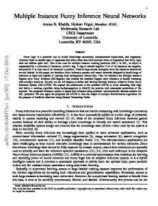
We propose using Multiple Instance Learning (MIL) as part of a two-level model, shown in Fig. 1. The first-level model is an Expectation Maximization (EM) based MIL method combined into a CNN that outputs patch-level predictions. In particular, we assume that there is a hidden 1

variable associated with each patch extracted from an image that indicates whether the patch is discriminative or not. Here, ”a patch being discriminative” means that the true hidden label of the patch is the same as the true label of the image. Initially, we consider all patches to be discriminative and train the CNN model that outputs the cancer type probability for each input patch. We apply a spatial smoothing to the resulting probability map and select only patches with higher probability values as discriminative patches. We iterate this process using the new set of discriminative patches in an EM fashion until convergence. In the second-level, the histogram of patch-level predictions is input into a multiclass logistic regression that predicts the image-level label.

active field of research and development. There are three major categories of algorithms and corresponding applications: Patch-level classification and/or segmentation methods [43, 8, 2, 34, 11] require that a lot of patch labels are provided. Certain methods [14, 25] integrate patchlevel information into supervised WSI classification. One method [25] uses a domain-specific pipeline for WSI-based Glioblastoma (GBM) vs. Low-Grade Glioma (LGG) classification and detects discriminative regions such as necrotic and microvascular proliferation areas are detected via a fully supervised model. This method then applies a decision tree for the final prediction of classes. The domainspecific discriminative features do not generalize to other cancer types, not even to subtype glioma classification. The need to integrate patch-level information without cancer type specific features led to MIL-based WSI classification [13, 37, 38, 19]. In the MIL paradigm [15, 24, 3], unlabeled instances belong to labeled bags of instances. The goal is to predict the label of a new bag and/or the label of each instance. The Standard Multi-Instance (SMI) assumption [15] states that for a binary classification problem, the bag is positive if and only if there exists at least one positive instance in the bag. This led to the MIL version of different classifiers [4, 41, 20], including MIL with Neural Networks (NN) [32, 44, 23]. The Back Propagation for Multi-Instance Problems (BP-MIP) [32, 44] performs back propagation along the instance with the maximum response if the bag is positive. This is inefficient because only one instance per bag is trained in one training iteration on the whole bag. An efficient neural network with MIL is proposed [23] with the drawback that it only works on the feature space due to the need of averaging over the instances. In image classification, the image is the bag and imagewindows are the instances [26]. Thus, MIL-based CNNs are applied to object recognition [28] and semantic segmentation [30]. In these methods, the training error is only propagated through the object-containing window which is also assumed to be the window that has maximum prediction confidence. We argue that this is not robust since training only on high-confidence windows may lead to overfitting. In recent semantic image segmentation approaches [9, 31, 29], a smoothing algorithm is applied on the output probability (feature) maps of CNNs. In this way, irrelevant windows can be identified more robustly. We generalized the previous idea and extended it to the patch-based image classification problem based on two assumptions: First, in each image, there may exist some nondiscriminative patches. Their true latent labels do not match the label of the image. Second, non-discriminative patches also contribute to the image-level labels jointly. For example [3], a beach image may contain a sand-patch and a water-patch; neither of them are by themselves beach

Figure 1: An overview of our workflow of glioma pathology image classification (best viewed in color). The assumption is that discriminative information is encoded in high resolution details and some of the patches extracted from the image do not contain such discriminative information. Top: An EM-based MIL-CNN that iteratively identifies non-discriminative patches and eliminates them from the training set. Bottom: The second-level model learns how to aggregate patch-level predictions to the image-level prediction. Pathology image classification and segmentation is an 2

patches. Based on these two assumptions, our method consists of two levels. The first-level model efficiently eliminates non-discriminative patches from the final CNN training whereas the second-level logistic regression predicts the image-level label based on the patch-level predictions [10]. The first layer model reduces the amount of noise and therefore improves performance. The second-level model models a more general multiple instance assumption [16] which fits the assumption of our main application of WSI-based glioma classification. It also can be interpreted as a stacked generalization method [36]. Our main contributions are as follows.

the bags are independent and identically distributed (i.i.d.), the X and the hidden variables H are generated by the following generative model: P (X, H) =

N Y

P (Xi | Hi )P (Hi )

i=1

=

N  Y

 P (Xi,1 , Xi,2 , . . . , Xi,Ni | Hi )P (Hi ) ,

i=1

(1) where the hidden variable H = {H1 , H2 , . . . , HN }, where Hi = {Hi,1 , Hi,2 , . . . , Hi,Ni } and Hi,j is the hidden variable that indicates whether instance xi,j is discriminative for label yi of bag Xi . We further assume that all Xi,j depends on Hi,j only and are independent with each other given Hi,j . Thus

1. We propose a new classification model that combines MIL with CNNs that work in raw pixel space. It utilizes the spatial relationship between patches extracted from image to identify discriminative patches. Additionally, our algorithm adds very little computational cost to the conventional supervised CNNs.

P (X, H) =

2. We propose a second-level model that can be applied on datasets that do not meet the SMI assumption. On the glioma classification dataset, this method outperforms the first-level model with the SMI assumption significantly.

Ni  N Y Y

 P (Xi,j | Hi,j )P (Hi ) .

(2)

i=1 j=1

We maximize the data likelihood P (X) using the EM algorithm. 1. At the initial E step, we set Hi,j = 1 for all i, j. This means that all instances are considered discriminative.

3. Our model achieves state-of-the-art results classifying Glioblastoma (GBM) and Low-Grade Glioma (LGG) on the TCGA dataset. Furthermore, for the first time, we can classify three major subtypes of LGG with an accuracy similar to inter-observer agreement between experienced pathologists.

2. M step: We update the model parameter θ to maximize the data likelihood

θ ← arg max P (X | H; θ) θ Y = arg max P (xi,j , yi | θ)

The rest of this paper is organized as follows. Sec. 2 describes the framework of the EM-based MIL algorithm. Sec. 3 discusses the identification of discriminative patches. Sec. 4 explains the second-level model that predicts the image-level label by aggregating patch-level predictions. Sec. 5 shows experimental results. The paper concludes in Sec. 6. App. A gives glioma subtype details.

θ

xi,j ∈D

Y

×

(3)

P (xp,q , yq | θ),

xp,q 6∈D

where D is the set of discriminative patches. We assume a uniform generative model for all nondiscriminative instances. Therefore the optimization problem in Eq. 3 can be simplified to

2. EM-based MIL with CNN An overview of our EM-based method can be found in Fig. 1. We model the high resolution image or video as a bag and the patches extracted from it as instances. We have a ground truth label for the whole image but not for the individual patches. Assuming some instances are not discriminative, i.e. the true label of the instances does not match the label of the bag, whether an instance is discriminative or not is modeled as a hidden binary variable. We denote X = {X1 , X2 , . . . , XN } as the dataset containing N bags. Each bag Xi = {Xi,1 , Xi,2 , . . . , Xi,Ni } consists of Ni instances, where Xi,j = hxi,j , yi i is the j-th instance and its associated label in the i-th bag. Assuming

arg max

Y

θ

xi,j ∈D

= arg max θ

Y

P (xi,j , yi | θ) (4) P (yi | xi,j ; θ)P (xi,j ).

xi,j ∈D

Additionally we assume a uniform distribution over xi,j . Thus Eq. 4 describes a discriminative model (in this paper we use a CNN). 3

3. E step: We estimate the hidden variables H. In particular, Hi,j = 1 if and only if P (Hi,j | X) is above a certain threshold. In the case of image classification, given the i-th image, P (Hi,j | X) is obtained by applying Gaussian smoothing on P (yi | xi,j ; θ) (Detailed in Sec 3). This smoothing step utilizes the spatial relationship of P (yi | xi,j ; θ) in the image. We then iterate back to the M step till convergence.

patches that are considered discriminative for each image. Second, by using the class-level threshold, the thresholds can be easily adapted to classes with different prior probabilities. Layer Input Conv ReLU+LRN Max-pool Conv ReLU+LRN Max-pool Conv ReLU Conv ReLU Max-pool FC ReLu+Drop FC ReLu+Drop FC Softmax

Many MIL algorithms can be interpreted as a version of this formulation. Based on the SMI assumption, the instance with the maximum P (Hi,j | X) is considered as the discriminative instance for the positive bag, as in the EM Diverse Density (EM-DD) [42] and the BP-MIP [32, 44] algorithms. In the latter case, a single gradient descent is performed in the M step per positive bag, which makes the algorithm computationally inefficient. In the field of semantic image segmentation, [29] uses a fully connected Conditional Random Field (CRF) to model P (H | X) and then perform the relevant EM-based updates.

3. Discriminative instance selection This section focuses on the E step of estimating P (H | X) and the way to choose a threshold for determining whether a patch is discriminative. After this step, the patches xi,j that have P (Hi,j | X) larger than a threshold Ti,j are considered as discriminative and are selected to continue training the CNN. To estimate P (Hi,j | X), it is straightforward to assume that P (Hi,j | X) is correlated with P (yi | xi,j ; θ), i.e. patches with lower P (yi | xi,j ; θ) tend to have lower probability xi,j to be discriminative. However, a hard-to-classify patch, or a patch close to the decision boundary may have low P (yi | xi,j ; θ) as well. These patches are informative and should not be rejected as non-discriminative. Therefore, to obtain a more robust P (Hi,j | X), we apply the following two steps: First, we train two CNNs on two different scales in parallel and the prediction P (yi | xi,j ; θ) is the averaged prediction of the two CNNs. Second, we simply denoise the probability map P (yi | xi,j ; θ) of each image with a Gaussian kernel to obtain P (Hi,j | X). Choosing a thresholding scheme carefully yields significantly better performance than a simpler thresholding scheme [29]. We obtain the threshold Ti,j for P (Hi,j | X) as follows: We note Si as the set of P (Hi,j | X) values for all xi,j of the i-th image and Ec as the set of P (Hi,j | X) values for all xi,j of the c-th class. We introduce the imagelevel threshold Hi as the P1 -th percentile of Si and the class-level threshold Ri as the P2 -th percentile of Ec , where P1 and P2 are predefined parameters. Then the threshold Ti,j is defined as the minimum value between Hi and Ri . There are two advantages of our method. First, by using the image-level threshold, there are at least 1 − P1 percent of

Filter size, stride 10 × 10, 2 6 × 6, 4 5 × 5, 1 3 × 3, 2 3 × 3, 1 3 × 3, 1 3 × 3, 2 -

Output size 400 × 400 × 3 196 × 196 × 80 196 × 196 × 80 49 × 49 × 80 45 × 45 × 120 45 × 45 × 120 22 × 22 × 120 20 × 20 × 160 20 × 20 × 160 18 × 18 × 200 18 × 18 × 200 9 × 9 × 200 320 320 320 320 6 6

Table 1: The architecture of our CNN used in glioma classification. The output size is given in width × height × the number of feature maps. ReLU+LRN is a sequence of Rectified Linear Units (ReLU) followed by Local Response Normalization (LRN). Similarily, ReLU+Drop is a sequence of ReLU followed by dropout. The dropout probability is 0.5.

4. Image label prediction In this section we describe how we combine the patchlevel classifiers of Sec. 3 to predict accurately the imagelevel label. We input all the predictions of the patch-level classifiers into a multi-class logistic regression that predicts the image-level label. There are two reasons for combining multiple instances: First, on difficult datasets, we do not want to assign an image-level prediction just based simply based on a single patch-level prediction (as is the case of the SMI assumption [15]). Second, even though certain patches are not discriminative individually, their joint appearance might be discriminative. For example, Oligoastrocytoma (OA) (see App. A) is a ”mixed” type glioma that is diagnosed when two single glioma types (Oligodendroglioma and Astrocytoma, possibly on different patches) are jointly present on the slide. In particular, the class histogram of the patch-level predictions is the input to our linear multi-class logistic regression model [6]. This model uses an L2 regularizer which is 4

sub-patch is selected, where S is a predefined hyperparameter. Second, the sub-patch is randomly rotated and mirrored. Third, the amount of Hematoxylin and eosin stained on the tissue is randomly adjusted. This is done by decomposing the RGB color of the tissue into H&E color space [33], followed by multiplying the magnitude of H and E of every pixel by two i.i.d. Gaussian random variables with expectation equal to one.

selected by cross-validation on a validation dataset. A linear model is sufficient in this case because the inputs of the model are expected to be directly correlated with the output labels. This model can be thought of a count-based multiple instance learning method with two-level learning [35].

5. Experiments We have evaluated our method on two datasets: The Cancer Genome Atlas (TCGA) dataset [1] for Whole Slide Image (WSI) based glioma classification and the Kinect interaction dataset [39] for two-person interaction classification.

5.1.3

Following previous work [21], the architecture of our CNN is shown in Tab. 1. We used the CAFFE tool box [18] for the CNN implementation. The network was trained on a single NVidia Tesla 40K GPU.

5.1. WSI-based glioma classification We have evaluated our algorithm to the glioma classification problem on the TCGA dataset. Based on large scale experiments we show that our model outperforms existing methods significantly. 5.1.1

5.1.4

The TCGA dataset contains detailed clinical information and the Hematoxylin and Eosin (H&E) stained WSIes of 6 types of gliomas. A typical resolution of a WSI is 100k by 50k pixels. Fig. 2 shows sample patches of each class. The numbers of WSIes and patients in each class are shown in Tab. 2. All classes are described in the App. A. # of WSIes 510 206 183 114 36 15

1. NM-LBP: Nuclei Morphological features [12] and rotation invariant Local Binary Patterns [27] are extracted from all the patches extracted from the image, followed by SVM with radial basis function kernel [7]. We report this as a non-CNN baseline.

# of patients 209 100 106 82 29 13

2. CNN-Vote: CNN followed by voting. Instead of training the second-level logistic regression, the final predicted label of the WSI is determined by voting from the prediction of all its patches.

Table 2: The numbers of WSIes and patients in each class from the TCGA dataset. For descriptions of each class, see the App. A.

5.1.2

Experiment setup

To test our method, WSIes of 80% of the patients are randomly selected to train the model and the remaining 20% for testing. Depending on the method, the training set is further divided into two parts randomly: the CNN training set and the logistic regression cross-validation set. The data separation is performed twice and the results are averaged. The algorithms tested are listed below.

TCGA dataset

Glioma GBM OD OA DA AA AO

CNN architecture

3. CNN-SMI: CNN followed by max-pooling. This method follows the SMI assumption. The final predicted label of the WSI equals to the predicted label of the patch with maximum probability over all other patches and classes.

Patch extraction and augmentation 4. CNN-LR: CNN followed by our second-level multiclass logistic regression to predict the image-level label. One tenth of the images is held out from the CNN to train the second-level multi-class logistic regression by 10-fold cross-validation.

To train the CNN model, patches of size 500 by 500 are extracted from the WSI. To capture structures in different scales, we extract patches from two scales: 20X (0.5 microns per pixel) and 5X (2.0 microns per pixel). Patches that contain less than 30% tissue sections or have too much blood are discarded. For each WSI, patch stride is computed carefully to make sure around 1000 valid patches per image per scale are extracted. Therefore, in most cases the patches are non-overlapping given the resolution of the WSI. To prevent the CNN from severe overfitting, we perform three kinds of data augmentation. First, a random S by S

5. EM-CNN-Vote: CNN-Vote with our EM-based MIL. The percentile for class-level threshold P1 = 5%. The percentile for image-level threshold P2 = 30%. See Sec. 3 for the description of these parameters. In each M step, the CNN is trained on all the discriminative patches for 2 epochs. 5

(a) GBM

(b) OD

(c) OA

(d) DA

(e) AA

(f) AO

Figure 2: Some 20X sample patches of 6 types of gliomas from the TCGA dataset. The two patches in each column belong to the same class. Notice the large intra-class heterogeneity. 6. EM-CNN-SMI: CNN-SMI with our EM-based MIL. Ground Truth GBM OD OA DA AA AO

7. EM-CNN-LR: CNN-LR with our EM-based MIL. 8. NS-CNN-LR: No Gaussian Smoothing is applied to estimate P (H | X). Other parts are the same as EMCNN-LR. Algorithms Chance NS-LBP CNN-Vote CNN-SMI CNN-LR EM-CNN-Vote EM-CNN-SMI EM-CNN-LR NS-CNN-LR

Accuracy 0.513 0.629 0.710 0.710 0.752 0.733 0.719 0.771 0.745

mAP 0.689 0.734 0.812 0.822 0.847 0.837 0.823 0.845 0.832

Training Hrs 32 210 210 201 243 243 240 225

OD 47 18 9 2 2

Predictions OA DA 2 22 2 40 8 6 20 3 3 3

AA 1 3

AO 1 1 1

4 1

Table 4: The confusion matrix of glioma classification. The Oligoastrocytoma introduces the most confusions due to its nature. See Sec. 5.1.5 for details.

first to classify automatically LGG subtypes, a much more challenging classification task than the benchmark GBM vs. LGG classification. We achieve 57.1% LGG-subtype classification accuracy with chance being 36.7%. Notice that there are more confusions related to Oligoastrocytoma (OA) because it is a mixed glioma that is challenging even for pathologists to agree on. An experiment showed that the inter-observer agreement of four experienced pathologists in a LGG-labeling task similar to the one we are attempting in this paper 1 was approximately 52% and that even after reviewing the cases together, they agreed only around 69% of the time [17]. We tried different patch sizes S and report training time as well and accuracy in Fig. 4. Examples of discriminative and non-discriminative patches identified by the E-step are shown Fig. 3.

Table 3: Glioma classification results. All algorithms in this table use multiscale patches (5X and 20X). The proposed method EM-CNN-LR outperforms CNN-Vote and CNNSMI significantly.

5.1.5

GBM 214 1 1 3 3 2

Results

The results of our experiments are shown in Tab. 3. The confusion matrix is given in Tab. 4. From the confusion matrix, we observe that classification accuracy between GBM and LGG is 97% (chance was 51.3%). A fully supervised method achieved 85% accuracy using a domain specific algorithm trained on ten manually labeled patches per class [25]. To the best of our knowledge our method is the

1 Our results are not directly comparable due to different composition of datasets.

6

(a) GBM

(b) OD

(c) OA

40K GPU. The accuracy of the interaction classification is shown in Table 5. An analysis of the non-discriminative frame identification results is given in Figure 5. Since this is an “easy” dataset, CNN performance is already high and so our EM-based method does not improve them further in this dataset. Nevertheless, it identifies non-discriminative patches effectively. Since there is no evidence showing that non-discriminative frames would contribute to the videolevel label in this dataset, there is no need to apply a secondlevel logistic regression. In contrast, for the glioma classification task, a WSI of OA may contain two unoverlapping regions of different gliomas (See App. A); therefore, patches from these two regions decide the image-level label jointly, and the second level LR is essential.

(d) DA

Figure 3: Examples of automatically identified discriminative (first row) and non-discriminative (second row) patches of four glioma types.

Algorithms Chance MILBoost MILBoost clean SVM Linear SVM Linear clean CNN-Vote CNN-SMI CNN-LR EM-CNN-Vote EM-CNN-SMI EM-CNN-LR

0.78 0.76

Accuracy

0.74 0.72 200p 5X EM−CNN−LR 200p 20X EM−CNN−LR 400p 5X EM−CNN−LR 400p 20X EM−CNN−LR 400p multiscale CNN−LR 400p multiscale EM−CNN−LR

0.7 0.68 0.66 1

2

3

4

5

6

Days of Training

7

8

9

10

Accuracy 0.165 0.873 0.911 0.687 0.876 0.926 0.920 0.803 0.923 0.931 0.824

Table 5: The results of two-person interaction classification. The SVM and MILBoost algorithm [41] uses skeleton features extracted from the RGB-D frames [40]. Notice that CNNs on the noisy dataset already outperfom MILBoost on the clean dataset (MILBoost clean). See text for details.

Figure 4: Training time and results for different sizes of patches. Note that the multiscale settings and EM-based approaches increase accuracy significantly.

5.2. Two-person interaction classification

6. Conclusions

We performed an additional experiment on the SBU Kinect interaction dataset [40], a less challenging, well understood dataset, both as a sanity check and to test the applicability of our method to other types of large scale, hard to annotate precisely image-based data. The goal of the dataset is to detect two-person interaction activities in RGBD videos. We use the noisy version of the dataset [40]. Compared to the clean version, each video segment contains five more frames at both its start and end. In total 260 video segments of eight two-person interaction types are provided: “approaching”, “departing”, “kicking”, “punching”, “pushing”, “hugging”, “shaking hands”, and “exchanging”. The classification task is an MIL problem because some of the frames do not contain the labeled video-level actions. To train the CNN model, we only use depth frames. The architecture of our CNN is similar to that in Table 1 but has much smaller filters and fewer feature maps. The training error converges in a few hours on a single NVidia Tesla

We proposed a Multiple Instance Learning (MIL) based Convolutional Neural Network (CNN) model with a second-level logistic regression that can be applied to high resolution image classification. In this method, we assume that images are too large to apply CNN on whole images. On the other hand, patches extracted from an image may not be discriminative. Thus we follow a Multiple Instance Learning paradigm. We model whether a patch is discriminative or not by a hidden variable and apply EM to maximize the data likelihood. There are two key ideas of our algorithm. First, a spatial prior regularizes the hidden variables. Second, the second-level model is applied on datasets that do not meet the Standard Multiple Instance (SMI) assumption. With our algorithm, we can classify three major subtypes of Low-Grade Glioma (LGG) with an accuracy similar to inter-observer agreement between experienced pathologists. As part of future work we plan to lever7

# of identified irrelevant frames

300

II.

NS-CNN-SMI 250

3. OA: Oligoastrocytoma, ICD-O 9382/3, WHO grade II; and Anaplastic oligoastrocytoma, ICD-O 9382/3, WHO grade III. These two subtypes are mixed in one class because they have the same International Classification of Diseases for Oncology (ICD-O) code. Also, the two subtypes are both mixed gliomas of OD and DA. In other words, a WSI of OA may contain two distinct regions of OD and DA. OA is very hard to classify even by pathologists [17].

EM-CNN-SMI

200 150 100 50 0 0

5 10 15 20 25 # of frames away from the start or the end of the video

30

4. DA: Diffuse astrocytoma, ICD-O 9400/3, WHO grade II.

Figure 5: The localization of identified non-discriminative (irrelevant) frames. The identified non-discriminative frames which do not contain the labeled video-level action are concentrated at either the start or end of the video. This phenomenon is clearer if temporal Gaussian smoothing is applied (EM-CNN-SMI) compared to the algorithm without smoothing (NS-CNN-SMI). In this noisy version of the two-person interaction dataset, each video segment contains five more frames at both its start and end. Therefore, the non-discriminative frames are detected at the two ends of the video as expected, which acts as a sanity check for our claim of detecting non-discriminative frames.

5. AA: Anaplastic astrocytoma, ICD-O 9401/3, WHO grade III. 6. AO: Anaplastic oligodendroglioma, ICD-O 9451/3, WHO grade III.

References [1] The cancer genome atlas. https://tcga-data.nci. nih.gov/tcga/. [2] D. Altunbay, C. Cigir, C. Sokmensuer, and C. GunduzDemir. Color graphs for automated cancer diagnosis and grading. Biomedical Engineering, IEEE Transactions on, 57(3):665–674, 2010. [3] J. Amores. Multiple instance classification: Review, taxonomy and comparative study. Artificial Intelligence, 201:81– 105, 2013. [4] S. Andrews, I. Tsochantaridis, and T. Hofmann. Support vector machines for multiple-instance learning. In NIPS, pages 561–568, 2002. [5] Y. Bengio, A. Courville, and P. Vincent. Representation learning: A review and new perspectives. PAMI, 35(8):1798–1828, 2013. [6] C. M. Bishop et al. Pattern recognition and machine learning, volume 4. 2006. [7] C.-C. Chang and C.-J. Lin. Libsvm: a library for support vector machines. ACM Transactions on Intelligent Systems and Technology (TIST), 2(3):27, 2011. [8] H. Chang, Y. Zhou, A. Borowsky, K. Barner, P. Spellman, and B. Parvin. Stacked predictive sparse decomposition for classification of histology sections. International Journal of Computer Vision, pages 1–16, 2014. [9] L.-C. Chen, G. Papandreou, I. Kokkinos, K. Murphy, and A. L. Yuille. Semantic image segmentation with deep convolutional nets and fully connected crfs. arXiv preprint arXiv:1412.7062, 2014. [10] Z. Chen, Z. Chi, H. Fu, and D. Feng. Multi-instance multilabel image classification: A neural approach. Neurocomputing, 99:298–306, 2013. [11] D. C. Cires¸an, A. Giusti, L. M. Gambardella, and J. Schmidhuber. Mitosis detection in breast cancer histology images with deep neural networks. In MICCAI, pages 411–418. 2013.

age the non-discriminative patches as part of the dataset. We will explore soft assignments of for the probability that a patch is discriminative. We also plan to test our method with images from other cancer types.

Appendices A. Description of gliomas in the TCGA dataset The Cancer Genome Atlas (TCGA) project has whole slide tissue images from glioblastoma multiforme (GBM) and lower grade glioma (LGG) patients. Gliomas are differentiated into grades and sub-categories based on pathologic evaluation of tissues. This evaluation includes assessment of cell characteristics (such as shape and texture) as well as tissue region characteristics (such as existence of necrotic regions). Below is the list of glioma grades and subtypes available at the TCGA repository. 1. GBM: Glioblastoma, ICD-O 9440/3, WHO grade IV. GBM is the high grade glioma that are mostly found in cerebral hemispheres. A Whole Slide Image (WSI) is classified as GBM if and only if one patch can be classified as GBM with high confidence by a pathologist. 2. OD: Oligodendroglioma, ICD-O 9450/3, WHO grade 8

[28] M. Oquab, L. Bottou, I. Laptev, and J. Sivic. Weakly supervised object recognition with convolutional neural networks. [29] G. Papandreou, L.-C. Chen, K. Murphy, and A. L. Yuille. Weakly-and semi-supervised learning of a dcnn for semantic image segmentation. arXiv preprint arXiv:1502.02734, 2015. [30] D. Pathak, E. Shelhamer, J. Long, and T. Darrell. Fully convolutional multi-class multiple instance learning. arXiv preprint arXiv:1412.7144, 2014. [31] P. O. Pinheiro and R. Collobert. Weakly supervised semantic segmentation with convolutional networks. arXiv preprint arXiv:1411.6228, 2014. [32] J. Ramon and L. De Raedt. Multi instance neural networks. 2000. [33] A. C. Ruifrok and D. A. Johnston. Quantification of histochemical staining by color deconvolution. Analytical and quantitative cytology and histology/the International Academy of Cytology [and] American Society of Cytology, 23(4):291–299, 2001. [34] T. H. Vu, H. S. Mousavi, V. Monga, U. Rao, and G. Rao. Dfdl: Discriminative feature-oriented dictionary learning for histopathological image classification. arXiv preprint arXiv:1502.01032, 2015. [35] N. Weidmann, E. Frank, and B. Pfahringer. A two-level learning method for generalized multi-instance problems. In Machine Learning: ECML 2003, pages 468–479. 2003. [36] D. H. Wolpert. Stacked generalization. Neural networks, 5(2):241–259, 1992. [37] Y. Xu, T. Mo, Q. Feng, P. Zhong, M. Lai, E. I. Chang, et al. Deep learning of feature representation with multiple instance learning for medical image analysis. In ICASSP, pages 1626–1630, 2014. [38] Y. Xu, J.-Y. Zhu, I. Eric, C. Chang, M. Lai, and Z. Tu. Weakly supervised histopathology cancer image segmentation and classification. Medical image analysis, 18(3):591– 604, 2014. [39] K. Yun, J. Honorio, D. Chattopadhyay, T. L. Berg, and D. Samaras. Two-person interaction detection using bodypose features and multiple instance learning. In CVPR Workshop, 2012. [40] K. Yun, J. Honorio, D. Chattopadhyay, T. L. Berg, and D. Samaras. Two-person interaction detection using bodypose features and multiple instance learning. In CVPR Workshop, pages 28–35, 2012. [41] C. Zhang, J. C. Platt, and P. A. Viola. Multiple instance boosting for object detection. In NIPS, pages 1417–1424, 2005. [42] Q. Zhang and S. A. Goldman. Em-dd: An improved multiple-instance learning technique. In NIPS, pages 1073– 1080, 2001. [43] Y. Zhou, H. Chang, K. Barner, P. Spellman, and B. Parvin. Classification of histology sections via multispectral convolutional sparse coding. In CVPR, pages 3081–3088, 2014. [44] Z.-H. Zhou and M.-L. Zhang. Neural networks for multiinstance learning. In Proceedings of the International Conference on Intelligent Information Technology, pages 455– 459, 2002.

[12] L. A. Cooper, J. Kong, D. A. Gutman, F. Wang, J. Gao, C. Appin, S. Cholleti, T. Pan, A. Sharma, L. Scarpace, et al. Integrated morphologic analysis for the identification and characterization of disease subtypes. Journal of the American Medical Informatics Association, 19(2):317–323, 2012. [13] E. Cosatto, P.-F. Laquerre, C. Malon, H.-P. Graf, A. Saito, T. Kiyuna, A. Marugame, and K. Kamijo. Automated gastric cancer diagnosis on h&e-stained sections; ltraining a classifier on a large scale with multiple instance machine learning. In SPIE Medical Imaging, pages 867605–867605, 2013. [14] A. Cruz-Roa, A. Basavanhally, F. Gonz´alez, H. Gilmore, M. Feldman, S. Ganesan, N. Shih, J. Tomaszewski, and A. Madabhushi. Automatic detection of invasive ductal carcinoma in whole slide images with convolutional neural networks. In SPIE Medical Imaging, pages 904103–904103, 2014. [15] T. G. Dietterich, R. H. Lathrop, and T. Lozano-P´erez. Solving the multiple instance problem with axis-parallel rectangles. Artificial intelligence, 89(1):31–71, 1997. [16] J. Foulds and E. Frank. A review of multi-instance learning assumptions. The Knowledge Engineering Review, 25(01):1–25, 2010. [17] M. Gupta, A. Djalilvand, and D. J. Brat. Clarifying the diffuse gliomas an update on the morphologic features and markers that discriminate oligodendroglioma from astrocytoma. American journal of clinical pathology, 124(5):755– 768, 2005. [18] Y. Jia, E. Shelhamer, J. Donahue, S. Karayev, J. Long, R. Girshick, S. Guadarrama, and T. Darrell. Caffe: Convolutional architecture for fast feature embedding. arXiv preprint arXiv:1408.5093, 2014. [19] M. Kandemir, C. Zhang, and F. A. Hamprecht. Empowering multiple instance histopathology cancer diagnosis by cell graphs. In MICCAI, pages 228–235. 2014. [20] M. Kim and F. Torre. Gaussian processes multiple instance learning. In ICML, pages 535–542, 2010. [21] A. Krizhevsky, I. Sutskever, and G. E. Hinton. Imagenet classification with deep convolutional neural networks. In NIPS, pages 1097–1105, 2012. [22] Y. LeCun, L. Bottou, Y. Bengio, and P. Haffner. Gradientbased learning applied to document recognition. Proceedings of the IEEE, 86(11):2278–2324, 1998. [23] C. H. Li, I. Gondra, and L. Liu. An efficient parallel neural network-based multi-instance learning algorithm. The Journal of Supercomputing, 62(2):724–740, 2012. [24] O. Maron and T. Lozano-P´erez. A framework for multipleinstance learning. NIPS, pages 570–576, 1998. [25] H. S. Mousavi, V. Monga, G. Rao, and A. U. Rao. Automated discrimination of lower and higher grade gliomas based on histopathological image analysis. Journal of pathology informatics, 6, 2015. [26] M. H. Nguyen, L. Torresani, F. De La Torre, and C. Rother. Weakly supervised discriminative localization and classification: a joint learning process. In ICCV, pages 1925–1932, 2009. [27] T. Ojala, M. Pietikainen, and T. Maenpaa. Multiresolution gray-scale and rotation invariant texture classification with local binary patterns. PAMI, 24(7):971–987, 2002.

9