whose truth values are 'unknown', while Belnap [1] proposed a four-valued ... lier work [10, 7], we identified a useful family of multiple-valued logics, known as the ... model, represented as a multiple-valued Kripke structure, and a temporal ...
1
Efficient Multiple-Valued Model-Checking Using Lattice Representations (This is an extended version of the paper that appeared in CONCUR’01, August 2001.) Marsha Chechik, Benet Devereux, Steve Easterbrook, Albert Y.C. Lai, and Victor Petrovykh Department of Computer Science, University of Toronto, Toronto, ON M5S 3G4, Canada. Email: chechik,benet,sme,trebla,victor @cs.toronto.edu
f
g
Abstract. Multiple-valued logics can be effectively used to reason about incomplete and/or inconsistent systems, e.g. during early software requirements or as the systems evolve. We specify multiple-valued logics using finite lattices. In this paper, we use lattice representation theory to cast the multiple-valued modelchecking problem in terms of symbolic operations on classical sets of states, provided the lattices are distributive. This allows us to partially reuse existing symbolic model-checking technology and improve efficiency over previous implementations that were based on multiple-valued decision diagrams.
1 Introduction Multiple-valued logics provide an interesting alternative to classical boolean logic for modeling and reasoning about systems. By allowing additional truth values, they support the explicit modeling of uncertainty and disagreement. For these reasons, they have been explored for a variety of applications in databases [19], knowledge representation [20], machine learning [24], and circuit design [22]. A number of specific multi-valued logics have been proposed and studied. For example, Łukasiewicz [23] first introduced a three-valued logic to allow for propositions whose truth values are ‘unknown’, while Belnap [1] proposed a four-valued logic that also introduces the value ‘both’ (i.e. “true and false”), to handle inconsistent assertions in database systems. Each of these logics can be generalized to allow for different levels of uncertainty or disagreement. In practice, it is useful to be able to choose different multi-valued logics for different modeling tasks. The motivations that led to the development of these logics clearly apply to the modeling of software behaviour, especially the exploratory modeling used in the early stage of requirements engineering and architectural design. – We need to allow for uncertainty – for example, we may not yet know whether some behaviours should be possible; – We need to allow for disagreement – for example, different stakeholders may disagree about how the systems should behave; – We need to represent relative importance – for example, in the case where some behaviours are essential and others may or may not be implemented.
2 TT
T F
(a)
1T 0 0 1 0M 1 0 1 0F 1 0 1 (b)
TT
TT TF
(c)
FT FF
TF
UU FT
TM
TF
MT
MF
(d)
FF
(e)
FT
MM
FM FF
Fig. 1. (a) 2, the classical logic lattice; (b) 3, a 3-valued logic lattice, representing uncertainty; (c) 2x2, a 4-valued logic lattice, representing disagreement; (d) the 5-valued lattice, representing disagreement with “unknowns”; (e) a lattice 3X3.
For reasoning about dynamic properties of systems, existing modal logics can be extended to the multi-valued case. Fitting [17, 18] suggests two different approaches for doing this: the first extends the interpretation of atomic formulae in each world to be multi-valued; the second also allows multi-valued accessibility relations between worlds. The latter approach is more general, and our work on logic in this paper is somewhat similar to his. Three-valued logic has received most interest. It has been shown to be useful for analyzing programs using abstract interpretation [9, 25], and for analyzing partial models [3, 4]. Bruns and Godefroid also proved that automatatheoretic model-checking on 3-valued predicates reduces to classical model-checking. In our recent work [8], we showed that this result extends to many-valued logics, where the values form a total order (e.g., “True”, “Likely”, “Undecided”, “Unlikely”, “False”). Work has also been done on deciding a more general class of multi-valued logics. In particular, the work of H¨ahnle and others [21, 27] has led to the development of several theorem-provers for first-order multi-valued logics. This paper deals with symbolic model-checking for multi-valued logics. In our earlier work [10, 7], we identified a useful family of multiple-valued logics, known as the quasi-boolean logics [2] (or de Morgan logics [15]). A quasi-boolean logic has truth values that form a finite lattice, with a negation operator chosen such that the negation of each value is its image under horizontal symmetry. Conjunction and disjunction are defined as meet and join in the lattice, respectively. A few quasi-boolean logics are represented in Figure 1. Classical logic, referred to as 2, is given in Figure 1(a). The lattice in Figure 1(c) represents possible disagreement between two views: TT and FF represent unanimous agreement on true or false; TF and FT, two possible types of disagreement. The lattice in Figure 1(d) represents disagreement when some information is not known by either view. This sometimes happens when merging two partial views, represented by state machines. Suppose that a state s is present in one state machine, but a variable v is not. Suppose further that the variable v is present in the other state machine, but the state s is not. Then neither state machine can give the value for variable v in state s. Such situation requires introduction of a new logic value, “unknown”, represented in Figure 1(d) by value UU [16]. We are interested in building a model-checker that takes as its input a particular quasi-boolean logic, represented as a lattice of truth values (L; v), a state machine model, represented as a multiple-valued Kripke structure, and a temporal logic property expressed in CTL enriched with multiple-valued semantics, and returns the truth value that the property has in the initial state(s) and a counter-example, if applicable. Success of symbolic model-checking in a given domain (probabilistic, multiple-valued, timed, etc.) depends on being able to create efficient algorithms for manipulating the
3
sets of states in which a property holds. We need to calculate union, intersection, complement, and backwards reachability (for computing predecessors). For model checking in a given multiple-valued logic, we can treat these as operations over multiple-valued sets: sets whose membership functions are multiple-valued. We have explored a number of choices for efficient computation of these operations over multiple-valued sets in our previous work: – We can use MDDs, the multiple-valued extension of binary decision diagrams [5], as a canonical representation of the multiple-valued membership function. A multiplevalued model-checker based on MDDs is described in [7]. – We can represent the multiple-valued set as a collection of classical sets, one for each value of the logic. This approach has been taken in [10], using a MultipleValued Binary-Terminal Decision Diagram (MBTDD) [13] to represent each set. Clearly, multi-valued logics with a finite number of values do not add expressive power to the modeling. However, in many cases they produce a significantly smaller state space then the alternative approach of introducing additional boolean predicates. Still, the above approaches suffer from a fairly high running time (O(jLj3n � h � jpj, where h is the height of the lattice representing the logic, jLj is the number of logic values, jpj is the size of the formula under analysis, and n is the number of atomic propositions in the system), and we are interested in further optimizations of the modelchecker. In this paper, we describe a third alternative. We represent the multiple-valued sets as a collection of classical sets, but exploit a result of lattice theory to reduce the number of such sets that we need to represent. In a distributive lattice, any element of the lattice can be represented uniquely as the join of a subset of the join-irreducible elements of the lattice. This provides us with a compact encoding of the multiple-valued set membership function. This encoding supports efficient computation of the necessary set operations, and hence significantly reduces the running time of our model-checker. The paper is organized as follows: Section 2 introduces multiple-valued sets and multiple-valued set operations, whereas Section 3 shows how to represent these using join-irreducible elements of the lattice describing the logic. We review semantics of multiple-valued CTL and multiple-valued Kripke structures, and present the modelchecking algorithm in Section 4. We compare the performance of this model-checker with our previous multiple-valued model-checkers [7, 10] in Section 5 and conclude in Section 6.
2 Multiple-Valued Sets 2.1 Quasi-Boolean Logics Our approach to modeling makes use of an entire family of multi-valued logics. Rather than giving a complete axiomatization for each logic, we simply give a semantics by defining conjunction, disjunction and negation on the truth values of the logic, and restrict ourselves to logics where these operations are well-defined, and satisfy commutativity, associativity etc. Such properties can be easily guaranteed if we require that the truth values of the logic form a lattice. The partial order operation a v b means “b is at
4
T DK
DC UL VU F
Fig. 2. A finite distributive non-quasi-boolean lattice.
least as true as a”. Conjunction and disjunction of L are defined as u and t (meet and join) operations of (L; v), respectively. In defining negation, we decided that involution (::a = a) is essential, whereas the laws of non-contradiction (:a ^ a = ?) and excluded middle (:a _ a = >) are not. The resulting family of multiple-valued logics is known as quasi-boolean logics [2]. A quasi-boolean logic L has truth values that form a finite quasi-boolean lattice (L; v). Definition 1. A finite lattice (L; v) is quasi-boolean [2] if there exists a unary operator : defined for it, with the following properties (a; b are elements of (L, v)):
(a u b) = :a t :b (De Morgan) (a t b) = :a u :b
::a = a (: involution) a v b , :a w :b (: antimonotoni ) Thus, negation is defined as the : operator of (L; v). In this paper, we additionally assume that (L; v) is distributive, i.e., :
:
a t (b u ) = (a t b) u (a t )
a u (b t ) = (a u b) t (a u ) (distributivity)
Many lattices that we encounter in practice are distributive. For example, lattices in Figure 1(a),(b),(c),(e) are distributive. However, the lattice 5 in Figure 1(d) is not distributive1 . Furthermore, not all finite distributive lattices are quasi-boolean. Consider an example in Figure 2. This lattice also represents levels of disagreement: T, DK (“don’t know”), DC (“don’t care”), UL (“unlikely”), VL (“very unlikely”) and F. However, values UL and VL do not have counter-parts satisfying our definition of quasi-complement. 2.2 Definition of Multiple-Valued Sets We now define the concept of multiple-valued sets over quasi-boolean lattices and give their operations. In classical set theory, a set is defined by a boolean predicate, also called a membership function. Typically, it is written using set comprehension notation: a predicate P defines the set S = fx j P (x)g. For instance, if P = �x 2 Z : 0 � x � 10, then S is the set of all integers between 0 and 10 inclusive. If, instead of using a boolean membership function, we allow the membership function to range over a lattice, we obtain a multiple-valued set theory in which it is possible to make statements like “element x is more in set S than element y ”. We call the resulting sets mv-sets. Given a lattice L = (L; v), we define a multiple-valued set theory relative to it. For an mv-set S , and a candidate element x, we use S (x) to denote the membership degree of x in S . In the classical case, this amounts to representing a set by its characteristic function. 1
We address handling of these lattices in Section 6.
5 {1001,...,1999}
{1000}
{2000}
{...999,2001...}
Fig. 3. The 4-valued set of years in the second millennium.
We can use the 4-valued lattice representing disagreement (Figure 1(c)) to represent disagreement over membership of the set of years of the second millennium, as shown in Figure 3. In order to graphically depict an mv-set, we use the structure of its underlying lattice, but replace each element with the set of elements which take on that value in the mv-set. “Pedants” insist that a millennium begins on the year ending in 1, so to them 1000 is not in the set, but 2000 is. However, “partiers” wanted to celebrate the start of the third millennium in 2000, and so claimed that 1000 is in the second millennium, and 2000 is not. Let (v1 ,v2 ) represent the tuple of answers that Pedants and Partiers give to a question of membership of a given element in the second millennium. Then TT is the value for all elements of f1001, 1002, ..., 1999g, TF is the value for 2000 (Pedants say “yes”, whereas Partiers say “no”), FT is the value for 1000 (Pedants say “no”, whereas Partiers say “yes”), and they agree that no other years belong to the second millennium. We extend some standard set operations to the multiple-valued case by lifting the lattice meet and join operations, as follows: (S \L S 0 )(x) , (S (x) u S 0 (x)) (Multiple-valued intersection) (S [L S 0 )(x) , (S (x) t S 0 (x)) (Multiple-valued union) S = S 0 , 8x : (S (x) = S 0 (x)) (Extensional equality) It is easy to verify that if L is 2, the two-valued lattice representing classical logic (Figure 1(a)), then the membership function is a boolean predicate, and the set operations are simply standard set membership, union, and intersection. If L is the interval [0; 1℄, ordered by the usual � relation on real numbers, then we obtain fuzzy set theory [29]. The fuzzy-set lattice is infinite, but complete. Hence forward, we will restrict ourselves to finite and distributive quasi-boolean lattices. These are complete, so we can extend the notion of set complement to the multiple-valued case, by defining it in terms of the quasi-complement of L, and denoting it with a bar: S (x) , :(S (x)) (Multiple-valued complement) We then obtain the expected properties: S [L S 0 = S \ L S 0 (De Morgan 1) S \L S 0 = S [ L S 0 (De Morgan 2) S \L (T [L V ) = (S \L T ) [L (S \L V ) (Distributivity 1) S [L (T \L V ) = (S [L T ) \L (S [L V ) (Distributivity 2) Since our sets, either classical or multiple-valued, are subsets of some U , we denote the classical complement of a set S as U n S . For model-checking, U will be the set of all states of a model. We now define some additional concepts for mv-sets that are not needed in the classical set theory:
6
Definition 2. Support, Core, `-cut, and `-clip of a multi-valued set, S :
� (S ) , fx j S (x) 6= ?g C (S ) , fx j S (x) = >g *` (S ) , fx j ` v S (x)g +` (S ) , fx j S (x) v `g
(Support) (Core) (`-cut) (`-clip)
All of these operations create classical sets. Support, cut, and core are standard concepts from fuzzy set theory [29]; clip is a new operation, which we shall need to prove some later result. Following the conventions of fuzzy set theory, we identify an explicit universe of discourse U , rather than use an undefinable set of all possible entities. Mv-sets can be thought of as functions from elements of U to the underlying lattice; therefore, U =*?(S ). Consider the example 4-valued set of Figure 3. By inspection, we can see that C (S ) = f1001; : : : ; 1999g (all the years agreed on by both groups), � (S ) = f1000; : : : ; 2000g (all the years considered by either group), and *TF (S ) = f1001; : : : ; 2000g, the second millennium according to the Pedants. 2.3 Multiple-Valued Relations Now we extend the concept of degrees of membership in an mv-set to degrees of relatedness of two entities. This concept, formalized by multiple-valued relations, allows us to define multiple-valued transitions in a state machine models. Definition 3. A multiple-valued relation R on two sets S and T is an mv-subset of S � T . The forward image of an mv-subset Q of S under R is
F (R; Q) , �t:
G
s2S
(Q(s) u R(s; t))
and the backward image B (R; Q) of an mv-subset Q of T is
B (R; Q) , �s:
G
t2T
(Q(t) u R(s; t))
Given an mv-subset of S , its forward image under the relation R is an mv-subset of T ; likewise, an mv-subset of T has an mv-subset of S as a backward image.
3 Efficient Representations of Multiple-Valued Sets Having defined mv-sets, we now address an efficient implementation of the mv-set operations when the underlying lattice is finite and distributive. We represent each mvset compactly using the cuts of the join-irreducible elements in the lattice. In this section we review the concept of join-irreducibility and show that the join-irreducible encoding allows for efficient implementation of the mv-set operations and efficient recovery of the full mv-set.
7
3.1 Join-Irreducibility Definition 4. [12] An element j in L is join-irreducible iff j 6= ? and for any x and y in L, j = x t y implies j = x or j = y . Dually, an element m is meet-irreducible iff m 6= > and for any x and y , m = x u y implies m = x or m = y . In other words, j cannot be further decomposed into the join of other elements in the lattice, and m cannot be further decomposed into the meet of other elements in the lattice, just as prime numbers cannot be further factored into the product of other natural numbers. For example, the join-irreducible elements of the lattice 3x3 in Figure 1(e), shown in bold, are fMF, TF, FM, FTg. We denote the sets of all join-irreducible and meet-irreducible elements of a lattice L by J (L) and M(L), respectively. We will use join-irreducibility to provide us with a kind of “prime factorization” for mv-sets. Every lattice element of a finite lattice can be defined as a subset of joinirreducible elements: Theorem 1. [12] Let ` be any element in a lattice (L; v). Then ` = ` g. For example, in the latticeFshown in Figure 1(e), TT = F
MF; TF; FMg; FF =
f
;
F
F
f
j 2 J (L) j j v
MF; TF; FM; FTg; TM =
f
, and so on.
Lemma 1. [12] Let j , x, and y be elements of a distributive lattice (L; v), with j being join-irreducible. Then j v x t y iff j v x or j v y . Lemma 2. Let ` be any element of a quasi-boolean lattice (L; v). Then
x j x 2 L; ` v x g = f x j x 2 L; x v :` g
f:
The above two lemmas describe properties of join-irreducible elements that we exploit in our representation of mv-sets. Note that Lemma 1 only applies to distributive lattices, and Lemma 2 uses the : operator that we defined for quasi-boolean lattices. From here on we will assume all our lattices are distributive quasi-boolean lattices. Proofs for Lemma 2 and other non-trivial results appear in the Appendix. Definition 5. Let X be a subset of L. Then
max(X ) ,
�
if tX 2 X X unde ned otherwise
t
min(X ) ,
�
if uX 2 X uX unde ned otherwise
Definition 6. Up-sets and down-sets of lattice elements are defined as follows:
` , fx j x 2 L; ` v xg (Up-set of `) # ` , fx j x 2 L; x v `g (Down-set of `) "
8 {1000, 1002 ..., 2000}
{1001,...,1999}
{1000}
(a)
{}
{2000}
{...999,2001...}
{1002,..., 1998}
{}
(b)
{1001, 1003, ... 1999}
{1000}
(c)
{2000}
{1001, 1003, ... 1999}
Fig. 4. (a) The 4-valued set of years in the second millennium (same as Figure 3); (b) The even numbers between 1000 and 2000, represented as a 4-valued set; (c) The mv-intersection of the two sets.
3.2 Encoding mv-sets Using j -cuts Given that we can represent any element of a lattice using the join-irreducibles below it, we proceed to encode mv-sets using the collection of j -cuts for j 2 J (L). We will show that the j -cuts of an mv-set contain sufficient information to rebuild the original mv-set, and prove that all the necessary operations for symbolic model-checking – intersection, union, complement, and backward image – can be easily carried out in this encoding, provided the lattice is distributive. Our first result, which follows trivially from Theorem 1, states that the membership degree of an element in an mv-set is the join of all join-irreducibles whose cuts contain the element. Theorem 2. For any mv-set S with underlying lattice L,
S (x) =
G
j j j 2 J (L); x 2 *j(S )g
f
We now define the operations over mv-sets in terms of operations over their j -cuts. Theorem 3. The `-cut of a multiple-valued intersection is the intersection of the `-cuts of the individual mv-sets. For j 2 J (L), the j -cut of a multiple-valued union is the union of the j -cuts. 8` 2 L :*` (S \L T ) = *` (S )\ *` (T ) (Cut-intersection) 8j 2 J (L) :*j (S [L T ) = *j (S )[ *j (T ) (Cut-union) As an example, consider the two mv-sets shown in Figure 4, parts (a) and (b). The TF-cut of their mv-intersection should be the same as the (classical) intersection of the TF-cuts. By inspection, the TF-cut of part (a) is f1000; : : : ; 1999g, and that of part (b) is f1000; 1002; : : :; 2000g, with the intersection f1000; 1002; : : :; 1998g. The TF-cut of the mv-intersection of (a) and (b), shown in part (c), is f1000; 1002; : : :; 1998g, which is indeed the same as the intersection of the individual TF-cuts of these mv-sets. It is easy to check that the same holds for other j -cuts. Theorem 3 is the fundamental result that we will use throughout the remainder of this paper. Formulation of complementation uses two observations. First is a trivial corollary of Lemma 2, indicating that multiple-valued complement turns each j -cut into a :j -clip: Lemma 3. Each j -cut of an mv-set, S , is the :j -clip of the complement of S : *j
(S ) = +:j (S )
9
Second, every up-set of a join-irreducible, j , is the complement (in the lattice) of the down-set of some meet-irreducible m: Lemma 4. In all distributive lattices L = (L; v) there exists a bijection f : M(L) such that, for all join-irreducible j , " j = Ln # f (j ).
J
(L) !
It follows that for an mv-subset S of some universe U , *j (S ) = U n +f (j) (S ). We use this to construct the j -cut of a multiple-valued complement of an mv-set: Theorem 4. Let S be an mv-subset of some U , based on a lattice L = (L; v), and let j 2 J (L). The j -cut of the multiple-valued complement of S is the classical complement (in U ) of the f 1 (:j ) cut of S : *j (S ) = U n *f 1 (:j) (S ). Finally, we demonstrate that the j -cuts of the backward image of an mv-set under a multiple-valued relation are simply the backward images of the j -cuts of the relation: Theorem 5. Let R be a multiple-valued relation on S and T , and Q be an mv-subset of T , with the same underlying lattice. Then *j (B (R; Q)) = fs j (9t 2*j (Q) : (s; t) 2*j (R))g (Cut-reachability) These results allow us to represent each mv-set compactly as a family of its j -cuts. Theorem 2 guarantees that this representation of mv-sets preserves all information; it also tells us how to recover mv-set membership from the j -cuts. The advantage of this representation is in the computation of multiple-valued intersections and unions. If mv-sets were represented by families of pieces, i.e., indexed by 2 all lattice values, then intersection and union would both take as many as O(jLj ) classical set operations. In contrast, the cut-intersection and the cut-union theorems imply that our representation requires just O(jJ (L)j) classical set operations.
4 Multiple-Valued Model-Checking In this section we review multiple-valued Kripke structures, which we call �Kripke structures, and multiple-valued CTL (�CTL). We then outline a model-checking algorithm based on cuts of join-irreducible lattice values. 4.1 Semantics A state machine M is a �Kripke structure if M =(S; S0 ; R; I; A; L), where: – L is a quasi-boolean logic represented by a lattice (L, v). L provides the lattice for all mv-sets in the model. – A is a (finite) set of atomic propositions, otherwise referred to as variables. For simplicity, we assume that all variables are of the same type, with values ranging over the values of the logic L. – S is a (finite) set2 of states; each state is identified by a unique (within M ) label s. – S0 � S is the non-empty mv-set of initial states. 2
S is a classical set, but it can also be considered an mv-set where 8s : S (s) 2 f>; ?g.
10 [[a℄℄ , (I (s))(a) ^ ℄℄ , [['℄℄ \L [[ ℄℄ [[:'℄℄ , [['℄℄ [[' _ ℄℄ , [['℄℄ [L [[ ℄℄ [[EX'℄℄ , B (R; [['℄℄) [[AX'℄℄ , [[EX :'℄℄ [[E ['U ℄℄℄ , [[ ℄℄ [L ([['℄℄ \L [[EXE ['U [[A['U ℄℄℄ , [[ ℄℄ [L ([['℄℄ \L [[AXA['U [['
℄℄℄) ℄℄℄
\L [[EXA['U
℄℄℄
Fig. 5. Semantics of �CTL operators.
– R is the multiple-valued transition relation. For each state s, there is at least one (non-false) transition (s; t) 2 � (R), extending the classical notion of Kripke structures. – I is a labeling function that maps states in S to mv-subsets of A. Intuitively, for any symbol a 2 A, (I (s))(a) = ` can be considered equivalent to the variable a having value ` in state s. This description of �Kripke structures is that of our previous work [7], influenced by notation used for fuzzy transition systems [26]. Now we review the semantics of �CTL operators on a �Kripke structure M over a quasi-boolean logic L. In extending the CTL operators, we want to ensure that the expected CTL properties [11] are still preserved 3. The semantics of �CTL operators is given in Figure 5. We use the double-brace notation, adopted from denotational semantics, and write [['℄℄ to denote the mv-set of states representing a degree to which ' holds. The semantics of the EX operator comes from our previous definition of backward image (Definition 3). The definitions of AU , EU and AX are given using the properties of CTL operators [11]. 4.2 Multiple-Valued Model-Checking Algorithm Our multiple-valued model-checking algorithm is shown in Figure 6. In this algorithm, we encode state mv-sets and the transition relation for the model by their j -cuts. For mv-sets, we use the following shorthand:
'
, f*j ([['℄℄) j j 2 J (L)g (All j -cuts) '
j , *j ([['℄℄) (Single j -cut)
b b b b
The structure of this algorithm is based on our earlier algorithm in [10]. The routine
Che k(p) is the entry point, where p is the �CTL formula to be checked. It recurses
through p, associating each sub-formula ' with j -cuts (bb'
) of state mv-sets. The handling of ^ and _ follows from Theorem 3. The : operator is handled by the negation function, based on Theorem 4. The next-state operators EX and AX are handled by the pred function, based on Theorem 5; pred computes EX , and AX (') is obtained 3
Note that the AU fixpoint is somewhat unusual because it includes an additional conjunct, EXA['U ℄. This term preserves a “strong until” semantics for states that have no outgoing
> transitions in non-Kripke structures [6].
Che k(p)
11
2
case p A: case p = ': case p = ' :
:
b
return p return negation( ' )
b 8j 2 J (L) : b result j := b ' j \ b j return b result case p = ' _ : 8j 2 J (L) : b result j := b ' j [ b j return b result case p = AX ': return negation(pred(negation(b ' ))) case p = EX ': return pred(b ' ) case p = A['U ℄: return QUntil(A; b ' ; b ) case p = E ['U ℄: return QUntil(E; b ' ; b ) ^
negation(b ' )
8j 2 J (L) : b n j = S n (b ' neg[j ℄) b
return n
QUntil(Q; b ' ; b )
b QU := b repeat
b EXterm := pred(b QU ) if Q = A
b AXterm := negation(pred(negation(b QU )))
else
// Q = E
b AXterm := S 8j 2 J (L) : b QU j := b j [ (b ' j \ b EXterm j \ b AXterm j ) until b QU converges return b QU pred(b ' )
8j 2 J (L) : b result j := f s j 9t : t 2 b ' j ^ (s; t) 2 b R j g b result
return
Fig. 6. The model-checking algorithm.
from :EX (:'). Finally, EU and AU are fixpoints computed iteratively by the QUntil function using the equations given in Figure 5. In the negation function, a precomputed neg table is used for quick lookup of f 1 (:j ), for any join-irreducible element j , as required by Theorem 4. It is precomputed from the constructive proof of Lemma 4 where f is specified: first find f using f (j ) = max(Ln " j ), then fill in the neg table using neg[:f (j )℄ = j . Theorem 6. Given a �Kripke structure and a �CTL formula p to model-check, Che k(p) in the algorithm in Figure 6 returns bbp
, i.e., f*j ([[p℄℄) j j 2 J (L)g. 4.3 Running Times To determine the running time of this algorithm, we start by analyzing individual operations: union, intersection, complement and backward image. We use a Multiple-Valued Binary Terminal Decision Diagram (MBTDD) [13] to represent each j -cut, denoting
12 Operation and complement back. image
[
\
MBTDD-based
MDD-based
jJ (L)j � MBT(n)2 MDD(n)2 jJ (L)j � MBT(n) MDD(n) jJ (L)j � (MBT(n) + MBT(n) � MBT(2n)) MDD(n) + MDD(n) � MDD(2n)
Table 1. Running times for operations on mv-sets using MBTDDs with j -cut encoding vs. MDDs.
the size of a MBTDD for n variables as MBT(n). The running time of each operation on a Kripke structure is given in the middle column of Table 1, where n = jAj. For example, Theorem 3 allows us to do a pairwise union of each of J (L) j -cuts, taking jJ (L)j � MBT(n)2 operations. Computation of backward image for each of J (L) MBTDDs consists of a disjunction (MBT(n) operations) of conjunctions (Definition 3) between the formula (MBT(n)) and the transition relation (MBT(2n) operations). Next, note that the computation of QUntil in the model-checking algorithm in Figure 6 dominates the running time, with each state changing its position in bbQU
at most h times, where h is the height of the lattice (L; v), so the maximum number of iterations of the repeat-until loop is jS j � h. In each iteration, there are two pred operations, two negation operations, and three unions and intersections. In the worst case, MBT(n) = O(jLjjAj 1 ), so the running time of QUntil is O(jS j � h � jJ (L)j � jLj3jAj 2 ). Theorem 7. Given a �Kripke structure (S; S0 ; R; I; A; L) and a �CTL formula p, the 3jAj 2 algorithm in Figure 6 terminates in O(jpj � jS j � h � jJ (L)j � jLj ) time, where h is the height of the lattice.
5 Evaluation In this section, we compare the running time of the algorithm in this paper with those of our earlier algorithms [7, 10]. Since the structure of the algorithms does not change, the difference in performance is in the cost of the four operations on mv-sets: union, intersection, complement and backward reachability. In our first multiple-valued model-checker [10], we encoded each lattice value x as a sequence of jLj bits, where bit x was on if x 2 L, and off otherwise. In this paper, we encode a lattice value x using a bit for each j 2 J (L), which is on only when j v x. It is always better than the encoding in [10], and thus all operations are faster. The righthand column of Table 1 lists the running times of the four operations for the MDD-based representation of mv-sets that we used in [7]. We refer to the size of an MDD on n variables as MDD(n). Running times for MDD operations are similar to those for MBTDD operations; however, for a given mv-set, the MBTDDs representing the j -cuts are usually smaller than an MDD representing the whole mv-set. We can express the performance improvement of the model-checker in this paper in terms of the ratio between the average size of an MDD and that of an MBTDD for a given set of n variables, which we call . The performance improvements for the operations in Table 1 are jJ (L)j= 2 for unions and intersections, and at most jJ (L)j= for complements and backward images.
13
We can then assess the overall improvement by estimating for different types of problem. In the worst case, an MDD and an MBTDD can have the same number of non-terminal nodes, making roughly 1; then the algorithm of this paper actually results in a slowdown. However, our experience indicates that as problems get larger, approaches jLj. This improvement is because there are typically more common subexpressions in boolean-terminal diagrams than in their multi-terminal counterparts, and thus more possibility for sharing. Preliminary experimental results support this analysis. Results in Table 2 were produced by randomly generating a pool of sample functions of a given number of variables (3 to 6), and then creating the single MDD and the collection of jJ (L)j MBTDDs representing the function, and taking the average sizes of the individual decision diagrams over the sample. We give this issue a fuller treatment elsewhere [13]. Thus, we believe that there is a significant speedup when using the model-checking algorithm described in this paper. For unions and intersections this speedup can range from jLj to as much as jLj2 = log2 jLj, depending on the shape of the lattice. Number of variables Mean MDD size Mean MBTDD size Ratio ( ) 3 99 66 1.5 4 828 218 3.8 5 7,389 949 7.8 6 66,434 7,510 8.8 Table 2. Empirical results, for randomly-generated functions, with L = 3x3.
6 Conclusion The challenge for efficient model-checking over multiple-valued logics is to find a compact encoding for mv-sets of states that supports fast computation of mv-set union, intersection, complement and backwards reachability. In this paper we described an elegant solution based on the use of join-irreducible elements of a lattice to provide a factorization of the mv-sets. We demonstrated that this representation supports the necessary operations, and showed that the result is a significantly faster model-checking algorithm. The exact speedup depends on the size of the join-irreducible set. For example, when we multiply lattices, as we often do when reasoning about multiple points of view (with or without abstraction) [16], the size of the resulting join-irreducible set grows as the sum of sizes of join-irreducible sets of the original lattices. Furthermore, after casting the multiple-valued model-checking problem in terms of efficient operations on MBTDDs, we can further improve the running times by reusing existing symbolic model-checking technology. In particular, we can further optimize the MBTDD negation operation (to jJ (L)j) by using complement arcs, as in Somenzi’s CUDD library [28]. The use of join-irreducibility to optimize our algorithms introduces an important restriction on the logics that we can use in the model-checker. We originally chose to restrict ourselves to logics whose values form a quasi-boolean lattice, as these logics
14
behave similarly to classical logic, but do not enforce the law of excluded middle and the law of non-contradiction [10]. The optimization described in this paper restricts us further to logics whose lattices are distributive. Our motivation for developing a multiple-valued model-checker was to verify properties of models that contain uncertainty and/or disagreement [16]. For this we typically use the logics 3 and 2x2 (shown in Figure 1), and their products, all of which are distributive. However, when the logic is represented by a non-distributive lattice, e.g., 5, our model-checker automatically switches to the MDD-based algorithm, described in [7]. Thus, in the case where the optimization is possible, it is applied, and in the other cases, the more general algorithm is used. Optimizing model-checking on multi-valued logics through the use of join-irreducible elements is not restricted to branching-time logic or to symbolic model-checking. In particular, in our recent work [8] we showed that when all elements of the lattice are join-irreducible, then multi-valued model-checking reduces to several queries to a classical model-checker, and built a multi-valued LTL model-checker on top of SPIN.
Acknowledgments We would like to thank Alasdair Urquhart for suggesting that distributive lattices can be represented by their join-irreducible elements. This work was financially supported by NSERC and CITO.
References 1. N.D. Belnap. “A Useful Four-Valued Logic”. In Dunn and Epstein, editors, Modern Uses of Multiple-Valued Logic, pages 30–56. Reidel, 1977. 2. L. Bolc and P. Borowik. Many-Valued Logics. Springer-Verlag, 1992. 3. G. Bruns and P. Godefroid. “Model Checking Partial State Spaces with 3-Valued Temporal Logics”. In Proceedings of CAV’99, volume 1633 of LNCS, pages 274–287, 1999. 4. G. Bruns and P. Godefroid. “Generalized Model Checking: Reasoning about Partial State Spaces”. In Proceedings of CONCUR’00, volume 877 of LNCS, pages 168–182, August 2000. 5. R. E. Bryant. “Symbolic Boolean manipulation with ordered binary-decision diagrams”. Computing Surveys, 24(3):293–318, September 1992. 6. T. Bultan, R. Gerber, and C. League. “Composite Model Checking: Verification with Type-Specific Symbolic Representations”. ACM Transactions on Software Engineering and Methodology, 9(1):3–50, January 2000. 7. M. Chechik, B. Devereux, and S. Easterbrook. “Implementing a Multi-Valued Symbolic Model-Checker”. In Proceedings of TACAS’01, volume 2031 of LNCS, pages 404–419. Springer, April 2001. 8. M. Chechik, B. Devereux, and A. Gurfinkel. “Model-Checking Infinite State-Space Systems with Fine-Grained Abstractions Using SPIN”. In Proceedings of the 8th SPIN Workshop on Model Checking Software, volume 2057 of LNCS, pages 16–36. Springer, May 2001. 9. M. Chechik and W. Ding. “Lightweight Reasoning about Program Correctness”. CSRG Technical Report 396, University of Toronto, March 2000. 10. M. Chechik, S. Easterbrook, and V. Petrovykh. “Model-Checking Over Multi-Valued Logics”. In Proceedings of FME’01, volume 2021 of LNCS, pages 72–98. Springer, March 2001.
15 11. E. Clarke, O. Grumberg, and D. Peled. Model Checking. MIT Press, 1999. 12. B.A. Davey and H.A. Priestley. Introduction to Lattices and Order. Cambridge University Press, 1990. 13. B. Devereux. Symbolic representation and reasoning over state-based models with multiplicities. Master’s thesis, University of Toronto, Department of Computer Science, June 2001. 14. E.W. Dijkstra and C.S. Scholten. Predicate Calculus and Program Semantics. Springer, 1990. 15. J.M. Dunn. “A Comparative Study of Various Model-Theoretic Treatments of Negation: A History of Formal Negation”. In Dov Gabbay and Heinrich Wansing, editors, What is Negation. Kluwer Academic Publishers, 1999. 16. S. Easterbrook and M. Chechik. “A Framework for Multi-Valued Reasoning over Inconsistent Viewpoints”. In Proceedings of International Conference on Software Engineering (ICSE’01), pages 411–420, May 2001. 17. Melvin Fitting. “Many-Valued Modal Logics”. Fundamenta Informaticae, 15(3-4):335–350, 1991. 18. Melvin Fitting. “Many-Valued Modal Logics II”. Fundamenta Informaticae, 17:55–73, 1992. 19. Brian R. Gaines. “Logical Foundations for Database Systems”. International Journal of Man-Machine Studies, 11(4):481–500, 1979. 20. Matthew Ginsberg. “Multi-valued logic”. In M. Ginsberg, editor, Readings in Nonmonotonic Reasoning, pages 251–255. Morgan-Kaufmann Pub., 1987. 21. Reiner H¨ahnle. Automated Deduction in Multiple-Valued Logics, volume 10 of International Series of Monographs on Computer Science. Oxford University Press, 1994. 22. S. Hazelhurst. Compositional Model Checking of Partially Ordered State Spaces. PhD thesis, Department of Computer Science, University of British Columbia, 1996. 23. J. Łukasiewicz. Selected Works. North-Holland, Amsterdam, Holland, 1970. 24. R. S. Michalski. “Variable-Valued Logic and its Applications to Pattern Recognition and Machine Learning”. In D. C. Rine, editor, Computer Science and Multiple-Valued Logic: Theory and Applications, pages 506–534. North-Holland, Amsterdam, 1977. 25. M. Sagiv, T. Reps, and R. Wilhelm. “Parametric Shape Analysis via 3-Valued Logic”. In Proceedings of 26th Annual ACM Symposium on Principles of Programming Languages, 1999. 26. E. Santos. “Regular Fuzzy Expressions”. In Madan M. Gupta, George N. Saridis, and Brian R. Gaines, editors, Fuzzy Automata and Decision Processes, pages 169–176, New York, 1977. North–Holland. 27. Viorica Sofronie-Stokkermans. Automated theorem proving by resolution for finitely-valued logics based on distributive lattices with operators. Multiple-Valued Logic, 2000. 28. Fabio Somenzi. “Binary Decision Diagrams”. In Manfred Broy and Ralf Steinbr¨uggen, editors, Calculational System Design, volume 173 of NATO Science Series F: Computer and Systems Sciences, pages 303–366. IOS Press, 1999. 29. L.A. Zadeh. “Fuzzy Sets”. In R. R. Yager, S. Ovchinnikov, R. M. Tong, and H. T. Nguyen, editors, Fuzzy Sets and Applications: Selected Papers by L.A. Zadeh, pages 29–44, New York, 1987. John Wiley & Sons, Inc.
A
Appendix
In this appendix we give proofs for selected theorems appearing in the main body of the paper. The proofs follow the calculational style of [14].
16
Lemma 2. Let ` be any element of a quasi-boolean lattice (L; v). Then
x j x 2 L; ` v x g = f x j x 2 L; x v :` g
f:
Proof.
y 2 f :x j x 2 L; ` v x g ,
double negation
( y ) 2 f :x j x 2 L; ` v x g
: : ,
set specification
` v :y ,
negation is order-reversing; double negation
y v :` ,
set specification
y 2 f x j x 2 L; x v :` g
t u
Theorem 3. The `-cut of a multiple-valued intersection is the intersection of the `-cuts of the individual mv-sets. For j 2 J (L), the j -cut of a multiple-valued union is the union of the j -cuts. 8` 2 L :*` (S \L T ) = *` (S )\ *` (T ) (Cut-intersection) 8j 2 J (L) :*j (S [L T ) = *j (S )[ *j (T ) (Cut-union) Proof. We show both equations by set extensionality.
x 2*j (S [L T )
x 2*` (S \L T ) ,
Definition 2
,
multiple-valued intersection
,
Definition 2
,
multiple-valued union
` v (S \L T )(x)
j v (S [L T )(x)
` v S (x) u T (x) ,
lattice properties
,
,
j v S (x) t T (x) ,
Lemma 1
Definition 2 x 2*` (S ) and x 2*` (T )
,
Definition 2 x 2*j (S ) or x 2*j (T )
set theory
,
set theory
` v S (x) and ` v T (x)
j v S (x) or j v T (x)
x 2*` (S )\ *` (T )
x 2*j (S )[ *j (T )
Lemma 4. In all distributive lattices L = (L; v) there exists a bijection f : M(L) such that, for all join-irreducible j , " j = Ln # f (j ). Proof. Let f (j ) = max(Ln " j ) for any j has the claimed range, and is a bijection.
2 J
J
t u
(L) !
(L). We show that f is well-defined,
17
To see that f is well-defined, we let m = t(Ln " j ) and show that m This will give the appropriate definition for max (Definition 5).
2 Ln "
j.
m 2 Ln " j ,
set theory
m 2= " j ,
Definition 6
,
definition of m
j 6v m j 6v t(Ln " j ) The last expression holds because if we had j v t(Ln " j ), then by Lemma 1, induction, and finiteness of L, we would have j v x for some x 2 Ln " j , i.e., j v x such that j 6v x, which is a contradiction. Next, we show that f (j ) 2 M(L). We have f (j ) 6= > because > is in " j . Assume that f (j ) = a u b; we show that we will have f (j ) = a or f (j ) = b (Definition 4). Observe that j 6v a or j 6v b; otherwise, j v a u b = f (j ) (lattice properties), which is clearly a contradiction. Then it follows that f (j ) = a or f (j ) = b: j 6v a )
set theory and Definition 6
a 2 Ln " j )
definition of f (j )
a v f (j ) f (j ) = a u b v a by lattice properties a = f (j ) Similarly, j 6v b ) b = f (j ). )
Before proceeding, we remark that by mirroring the above argument, we can also define g : M(L) ! J (L) with g (m) = min(Ln # m). Now we show " j = Ln # f (j ) by set extensionality:
x 2 Ln # f (j ) ,
Definition 6
x 6v f (j ) ,
definition of f
,
lattice properties and contraposition
x 6v t(Ln " j ) x 2= Ln " j ,
double negation
x 2" j
Finally, we can show f (g (m)) = m and g (f (j )) = j , so that f is indeed a bijection. We will just show the former; the latter mirrors the argument. Let m 2 M(L), j = g (m), and m0 = f (j ); we show m0 = m by showing both m0 v m and m v m0 .
18
j = g (m) )
definition of g
j v u(Ln # m) ,
j = g (m)
lattice properties
)
x � x 2 Ln # m ) j v x
j 2 Ln # m
8 ,
Definition 6
,
x � x 6v m ) j v x
contraposition
,
x � j 6v x ) x v m
Definition 6
)
x � x 2 Ln " j ) x v m
8 ,
Definition 6
m 2 Ln " j
8 ,
Definition 6
j 6v m
8 ,
definition of g
lattice properties
lattice properties
m v t(Ln " j ) 0 , definition of m = f (j ) m v m0
j) v m 0 , definition of m = f (j ) 0 m vm Thus, f Æ g and g Æ f are identity functions and so f is a bijection. Therefore, we have shown that f : J (L) ! M(L), as constructed at the beginning of this proof, is a bijection and has the property " j = Ln # f (j ) for all j 2 J (L). u t (
t Ln "
Theorem 4. Let S be an mv-subset of some U , based on a lattice L = (L; v), and let j 2 J (L). The j -cut of the multiple-valued complement of S is the classical complement (in U ) of the f 1 (:j ) cut of S : *j (S ) = U n *f 1 (:j) (S ). Proof. *j
(S )
= Lemma 3 +:j (S ) = Involution +:j (S ) = Lemma 4 U n *f 1 (:j) (S ) t u
Theorem 5. Let R be a multiple-valued relation on S and T , and Q be an mv-subset of T , with the same underlying lattice. Then *j
(B (R; Q)) = fs j (9t 2*j (Q) : (s; t) 2*j (R))g (Cut-reachability)
19
Proof.
(B (R; Q)) = DefinitionGof B *j (�s : Q(t) u R(s; t)) *j
t2T
= Definition G 2 fs j j v ( Q(t) u R(s; t))g
t2T
= x v y u z , x v y; x v z fs j 9t 2 T : j v Q(t) u R(s; t)g = Lemma 1 fs j 9t 2 T : j v Q(t) ^ j v R(s; t)g = Definition of cut fs j 9t 2 T : t 2*j (Q) ^ (s; t) 2*j (R)g t u