Efficient network reconfiguration using minimum cost ... - Cristinel Ababei

IEEE TRANS. ON POWER SYSTEMS, THIS IS THE AUTHORS’ COPY. THE DEFINITIVE VERSION CAN BE FOUND AT IEEE.

1

Efficient Network Reconfiguration using Minimum Cost Maximum Flow based Branch Exchanges and Random Walks based Loss Estimations Cristinel Ababei, Member, IEEE, and Rajesh Kavasseri, Member, IEEE

Abstract—The efficiency of network reconfiguration depends on both the efficiency of the loss estimation technique and the efficiency of the reconfiguration approach itself. We propose two novel algorithmic techniques for speeding-up the computational runtime of both problems. First, we propose an efficient heuristic algorithm to solve the distribution network reconfiguration problem for loss reduction. We formulate the problem of finding incremental branch exchanges as a minimum cost maximum flow problem. This approach finds the best set of concurrent branch exchanges yielding larger loss reduction with fewer iterations, hence significantly reducing the computational runtime. Second, we propose an efficient random walks based technique for the loss estimation in radial distribution systems. The novelty of this approach lies in its property of localizing the computation. Therefore, bus voltage magnitude updates can be calculated in much shorter computational runtimes in scenarios where the distribution system undergoes isolated topological changes, such as in the case of network reconfiguration. Experiments on distribution systems with sizes of up to 10476 buses demonstrate that the proposed techniques can achieve computational runtimes shorter with up to 7.78× and with similar or better loss reduction compared to the Baran’s reconfiguration technique [1]. Index Terms—Computation time. Losses. Networks. Power distribution control.

I. I NTRODUCTION

N

ETWORK reconfiguration of power distribution systems is defined as the change in the network structure as a result of closing tie and opening sectionalizing switches. It has been identified as a primary mechanism that has a direct impact on reliability, efficient service restoration and maintenance of optimal operating conditions. For example, Consolidated Edison, the distribution utility of the City of New York, has proposed a third generation (G3) distribution network whose features include flexible reconfiguration, superfast simulators, advanced visualization tools, and adaptive response systems [2]. Such features are indispensable in fulfilling the vision of a self healing grid that can automatically respond to disturbances while continuously optimizing the overall performance. Electric Power Research Institute (EPRI)’s own endeavors to develop D-FSM (Distribution Fast Simulation and Modeling) [3] confirm the importance and need to develop a super-fast computational platform that can provide in real time information necessary to facilitate several This work was supported by the Department of Electrical and Computer Engineering at North Dakota State University (NDSU). C. Ababei and R. Kavasseri are with the Department of Electrical and Computer Engineering, NDSU, Fargo ND, 58108, USA (e-mail: [email protected]; [email protected])

distribution automation (DA) functions and system level lookahead capabilities. There are two fundamental challenges in the problem of reconfiguration of radial distribution systems. The first challenge is related to the combinatorial nature of the solution space: closing tie and opening sectionalizing switches yield a very large number of network topologies that need to be analyzed while seeking the optimal configuration. The second challenge is that the evaluation of each configuration requires the estimation of losses. Therefore, the efficiency of the network reconfiguration depends on both the efficiency of the loss estimation technique (which has to be used multiple times in order to evaluate loss reductions) and the efficiency of the reconfiguration approach itself. Both these tasks are computationally intensive and thus considerable research has been devoted in developing efficient algorithms [4]. In this paper, our goal is to address these problems by proposing a novel minimum cost maximum flow based reconfiguration algorithm and a novel random walks based loss estimation technique. We applied the proposed reconfiguration and loss estimation algorithms to systems with sizes of up to 10476 buses and achieved speed-ups of up to 7.78× compared to the Baran’s reconfiguration technique [1]. Preliminary results on the proposed reconfiguration method were reported in a conference paper [5]. In this paper, we additionally propose the random walks based loss estimation technique, combine the proposed algorithms to achieve further speed-up, and provide details of our implementations. The paper is organized as follows. Section II presents previous work related to network reconfiguration and loss estimation techniques. Section III describes the proposed minimum cost maximum flow based reconfiguration algorithm. Section IV describes the proposed random walks based loss estimation technique. Section V presents experimental results. Finally, this paper concludes with a summary in Section VI. II. R ELATED W ORK The network reconfiguration problem has been the subject of extensive previous research. Most of the previous work can be divided into three main categories: evolutionary and knowledge based techniques [6]-[10], heuristics [1],[11]-[15], and mixed methods [16],[17]. Even though evolutionary and knowledge based techniques can handle broader objectives, they suffer from very long computational runtimes and therefore are less suitable for online distribution automation. Hybrid reconfiguration approaches are mixed solutions that combine

IEEE TRANS. ON POWER SYSTEMS, THIS IS THE AUTHORS’ COPY. THE DEFINITIVE VERSION CAN BE FOUND AT IEEE.

evolutionary and heuristic techniques in order to shorten the computational runtime without sacrificing solution quality. Even though their runtimes are generally shorter than of evolutionary techniques, they are still computationally demanding compared to heuristics. Heuristic algorithms have been proven to offer excellent results with significantly shorter runtimes. Thus, they are among the best candidates for real time distribution system reconfiguration for loss minimization [18],[19]. For instance, Civanlar et al. [11] proposed an efficient reconfiguration algorithm based on the concept of branch exchange. The algorithm was later improved by Baran and Wu [1], who also proposed an algebraic expression to estimate loss reduction due to branch exchanges. Calculation of losses can be done if the power flow solution (PFS) is already available. However, the PFS calculation itself is a very computationally intensive task and has also been the subject of extensive previous research. Due to its nonlinear nature, numerical methods have been employed to obtain solutions with an acceptable tolerance. Most previous work on PFS techniques can be classified into Newton-Raphson based [20], compensation based [21], and forward/backward sweep based methods [22],[23]. The forward/backward sweep based method is simpler to implement and is more computationally efficient for solving radial systems. Such advantages may however disappear, compared to Newton-Raphson based methods, for heavy loaded systems and when voltage control devices are present in the system [24]. The forward/backward sweep based can efficiently estimate bus voltage magnitudes and real and reactive power values. Therefore, it can be used to calculate power losses. It has been used for voltage stability analysis [25] and adapted to handle mutual coupling [26]. III. M INIMUM C OST M AXIMUM F LOW BASED R ECONFIGURATION A. New Reconfiguration Algorithm The proposed network reconfiguration algorithm is an iterative heuristic algorithm. Its pseudocode description is presented in Fig. 1. Each iteration of the algorithm has two steps: (i) In the first step, losses are estimated using the routine Loss estimation technique(). For this, we use the DistFlow loss estimation technique studied in [22], which has been proven to be very efficient. (ii) In the second step, we search for incremental network changes that lead to large loss reductions. The novelty of our approach lies in the enhanced branch exchange technique employed for this search. Using a minimum cost maximum flow (MCMF) based modeling approach, we find sets of multiple branch exchanges that are implemented concurrently.

2

Algorithm 1: MCMF based reconfiguration algorithm 1: Reconfiguration() 2: Input: Distribution system, initial configuration, tie and sectionalizing switches, threshold (ǫ) 3: Output: Final configuration 4: iter ← 0; loss reduction ← ∞ 5: while loss reduction > ǫ do 6: iter ← iter + 1 7: Step 1: 8: Loss estimation technique() 9: Step 2: 10: - Construct flow network graph 11: - Solve MCMF problem 12: - MCMF sol. indicates set of branch exchanges 13: - Perform set of concurrent branch exchanges 14: - Compute loss reduction 15: end while Fig. 1. Pseudocode of the proposed network-flow based reconfiguration. Speed-up is achieved due to fewer iterations thanks to the MCMF modeling and due to the efficient random walks based loss estimation technique.

associated with switch 26 can be implemented by closing switch 26 and opening either switch 21 (load is transferred from feeder F4 to feeder F1 ) or switch 6 (load is transferred from F1 to F4 ). In order to increase the amount of loss reduction during one iteration of the reconfiguration algorithm, one can select to close two or more tie switches simultaneously. However, in order for the loss reduction estimates to remain accurate, these multiple branch exchanges have to be independent. Two branch exchanges are independent if they are between different feeders. For example, in Fig. 2, the branch exchange between feeders F1 ,F4 via the tie switch 26 is independent from the branch exchange between feeders F2 ,F3 via the tie switch 24. The key idea of our reconfiguration algorithm lies in the way we find the set of concurrent first-order branch exchanges. We do that by formulating this problem as a minimum cost maximum flow problem. This formulation includes the following steps, as described below: 1) Construction the flow network graph G(V, A). 2) Solve the MCMF problem. 3) Perform the set of branch exchanges as indicated by the solution of the MCMF problem. 1) Construction the Flow Network Graph: The construction of the flow network graph G(V, A), where V and A are the

B. Minimum Cost Maximum Flow Based Multiple Concurrent Branch Exchanges During each iteration of the proposed reconfiguration algorithm we search for multiple first-order branch exchanges that cumulatively offer a larger loss reduction compared to conventional single branch exchange based methods [1],[14]. A first-order branch exchange is achieved by closing a tie switch and opening the closest sectionalizing switch. For example, in Fig. 2, the two first-order branch exchanges

Fig. 2. Balanced one line diagram of an example distribution network with four feeders. For simplicity, the loads P, Q are not represented.

IEEE TRANS. ON POWER SYSTEMS, THIS IS THE AUTHORS’ COPY. THE DEFINITIVE VERSION CAN BE FOUND AT IEEE.

sets of nodes and arcs, is crucial to the correctness of the proposed technique. In order to easier describe this step we use the example in Fig. 2. The flow network graph is constructed using the following graph construction rules (the result of the application of these rules to the example from Fig. 2 is presented in Fig. 3): • The graph contains a source s node and a sink t node. • The graph contains donor feeder, acceptor feeder, and switch nodes. There can be up to 2F donor and acceptor feeder nodes and S switch nodes, where F is the number of feeders in the system and S is the number of tie switches. A donor feeder node is associated with a feeder tree, which will transfer load (i.e., donate) to another feeder tree, associated with an acceptor node. A switch node Su,v represents the closing of tie switch u and opening of sectionalizing switch v. • A pair of arcs from a donor feeder node Fi to an acceptor feeder node Fj via a switch node Su,v is created only if a load transfer from feeder Fi to feeder Fj leads to a loss reduction. The loss reduction value is used to compute the arc cost assigned to the first arc of the pair. Because we seek branch exchanges that lead to the largest loss reduction, the cost is inversely proportional to the loss reduction. All other arcs have a cost of zero and all arcs in the graph have a flow upper bound of 1. For example, in Fig. 3, the pair of arcs between feeders F1 and F2 via S22,2 represents a branch exchange. The loss reduction that would be achieved by this branch exchange is used to compute the cost of 9 assigned to arc (F1 , S22,2 ). • If a pair of arcs is created between feeders Fi and Fj via switch Su,v , then a pair of arcs between Fj and Fi through the same switch is prohibited. That is because loss reduction can be achieved in only one direction by closing a tie switch. • If there are more possible branch exchanges between two feeders Fi and Fj , only the one that leads to the maximum loss reduction is used in the graph construction. For example, in Fig. 2, even though there are two possible branch exchanges between feeders F1 ,F2 via switches 22 and 23, only the branch exchange via switch 22 (due to its larger loss reduction) is included during the graph construction from Fig. 3. 2) Solve the MCMF problem: After the flow network graph is constructed using the procedure described in the previous section, the minimum cost maximum flow problem can be formally written, using the terminology from [27], as follows: X M inimize cij xij (1) Subject to

X j:(i,j)∈A

(i,j)∈A

xij −

X

xji = b(i)

∀i ∈ V

j:(j,i)∈A

xij ∈ {0, 1}

∀(i, j) ∈ A

where xij is the flow through arc (i, j) ∈ A and can be 0 or 1 because all arcs have unit capacity and cij is the cost associated with each arc. Variable b(i) is the flow1 supply 1 Not

to be confused with the concept of power flow.

3

Fig. 3. Illustration of the flow network graph. Each arc in A is tagged with a (flow upper bound, cost) pair. The solution of the MCMF problem is highlighted using thicker arcs. A similar flow network is created during each iteration of the proposed MCMF based algorithm.

(demand) associated with node i ∈ V . In our formulation, b(i) is set only for the source and sink nodes. It is set to the minimum between the number of outgoing arcs from the source node and the number of incoming arcs into the sink node. For instance, in the flow network graph from Fig. 3, b(s) = 2 and b(t) = −2, which capture the fact that only two branch exchanges will be part of the solution. We solve this MCMF problem using an efficient implementation of the scaling push-relabel algorithm studied in [28]. 3) Perform Concurrent Branch Exchanges: The solution of the MCMF problem practically dictates all the concurrent branch exchanges that we select to be implemented during the current iteration. In other words, the flows in the network flow graph found by the MCMF solution represent the load transfer between feeders, via the corresponding switches along the paths of the flows. For example, the solution of the problem in Fig. 3 is highlighted by using thicker lines that indicate concurrent load transfers between feeders F1 → F4 and feeders F3 → F2 , which lead to maximum loss reduction. At the end of the current iteration, the power system is reconfigured by closing switches 26, 24 and opening switches 15, 6. This new configuration represents the starting configuration in the next iteration. IV. R ANDOM WALKS BASED L OSS E STIMATION FOR F URTHER R ECONFIGURATION S PEED UP In this section, we propose a novel random walks based technique for voltage magnitudes estimation in order to speed up the DistFlow loss estimation and therefore the reconfiguration algorithm. The parallel between random walks and resistive networks was proposed by [29]. It is a statistical method that interprets similarly conductances and probabilities. This idea was applied to the analysis of VLSI circuits [30]. In what follows we adapt it for the estimation of bus voltage magnitudes in radial distribution systems. A. Random Walks Based Bus Voltage Magnitude Estimation Based on the discussion on the parallel between radial networks and random walks presented in Appendix A, we propose to use the random walks technique for the computation of the bus voltage magnitudes. Because the Y matrix is symmetric

IEEE TRANS. ON POWER SYSTEMS, THIS IS THE AUTHORS’ COPY. THE DEFINITIVE VERSION CAN BE FOUND AT IEEE.

and diagonally dominant, one can construct a random walks problem whose solution represents the solution of equation (4). Normally, because the summation of the coefficients of Ej from equation (4) can become greater than 1 (even though the absolute value of each of these coefficients is smaller than 1), one has to use scaling factors for the probabilities in equation (5) during the construction of the random walks problem [32]. For a detailed discussion of the scaling factors, the reader is referred to [32]. To avoid possible numerical instability due to scaling factors with absolute values greater than one, the bus voltage magnitudes (Ek ) are estimated by: X |Yjk | |Ik | X |Ek |′ ≈ |Ej | + X (2) |yjk | |yjk | (k,j)∈Adj (k,j)∈Adj

(a)

(b)

(k,j)∈Adj

In other words, based on the parallel between equations (2) and (5) we construct and then solve the random walks problem as described in the previous section. The solution of the random walks problem will give the voltage magnitudes for all buses of the system. The difference between the voltage magnitudes computed using this technique and DistFlow is negligible (it does not affect the quality of the reconfiguration as observed through experimental results later on) and will always be bounded because the expression in equation (2) is smaller than the upper bound: X |Ik | |Yjk | X X |Ej | + (3) UB = | yjk | yjk | (k,j)∈Adj | (k,j)∈Adj

4

Fig. 4. (a) Two examples of random walks performed for the node 22 of the 33-bus system. First RW with length 17: 22, 21, 20, 21, 20, 21, 20, 19, 2, 3, 4, 3, 2, 19, 20, 19, 2, 1. Second RW with length 7: 22, 21, 20, 19, 20, 19, 2, 1. (b) Illustration of the partial RW based update of voltage magnitudes of the nodes directly affected by topology changes.

(k,j)∈Adj

Once the bus voltage magnitudes are computed using the proposed RW based technique, the real and reactive power values are computed using a single forward pass similar to the DistFlow method. Being just one pass, this step is also very efficient. Then, power losses can be immediately calculated using the voltage and power values. Hence, our approach can be seen as a hybrid technique, which computes voltage magnitudes using random walks and power values using one forward pass of DistFlow. B. Computational Runtime Discussion The computational runtime of the proposed RW based technique depends on (i) the length (hitting time) of the walks, which in turn depends on the depth2 from home nodes and (ii) the number of nodes to update. The CPU runtime of a random walk is directly proportional to the length of the walk. This can be seen in Fig. 5, where we plot the variation of the average length of the random walk (for a single node) and its CPU runtime as a function of depth. This variation was observed for all tested systems for a variety of nodes located at different depths. Therefore, one can shorten the CPU runtime by increasing the number of home nodes (Fig. 4.b). This will decrease the depth of nodes and shorten the hitting times of random walks. In our implementation, we do that by processing only neighboring nodes of first 2 The depth of a node is defined as the distance from the closest home node. For example, the depth of node 22 is five in the system example from Fig. 4.a.

Fig. 5. Variation of the average length (as number of steps) of a random walk as a function of depth for the system from Fig. 4.a. This variation was observed for all tested systems.

and second order of the nodes directly affected by topology changes. The rest of the nodes are treated as home nodes, whose number is therefore increased. The voltage magnitudes of these additional home nodes (from outside the updated neighborhoods) are available from the previous iterations. The approach in which we exploit this distinct property of localizing the computation of random walks is referred to as the partial RW based technique. In summary, the partial RW based technique for loss estimation is a hybrid approach with two steps: (1) Use random walks to compute locally voltage magnitudes for nodes within first and second order neighborhoods of the nodes that are directly affected by local network topology changes. Because these random walks perform localized computations, the runtime compared to the case of running a full DistFlow for all nodes will be significantly reduced. (2) Use one forward pass of DistFlow to compute active and reactive power values. Then, power losses can be immediately calculated using the voltage and power values. V. E XPERIMENTAL R ESULTS The proposed algorithms were implemented in C++ and simulations were performed on a Linux machine running on a 2.8 GHz Intel Quad processor with 2 GB memory. The experimental setup is shown in Fig. 6. In this setup, we run four different experiments: (1) In the first experiment,

IEEE TRANS. ON POWER SYSTEMS, THIS IS THE AUTHORS’ COPY. THE DEFINITIVE VERSION CAN BE FOUND AT IEEE.

5

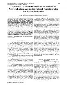
Fig. 7. Accumulated percentage of loss reduction achieved during iterations of the proposed algorithm and of Baran’s reconfiguration algorithm for the first testcase distribution system bus 83. Fig. 6.

Block diagram of the experimental setup.

which represents the reference for our comparisons, we run the traditional Baran’s reconfiguration method [1]. In this run, the traditional DistFlow technique is used for loss estimations. (2) In the second experiment, we run the proposed MCMF based reconfiguration algorithm. The traditional DistFlow is again used as the loss estimation technique. Hence, in this experiment, we will quantify the speed-up of the proposed MCMF based reconfiguration versus the Baran’s reconfiguration method from the first experiment. (3) In the third experiment, we use the traditional Baran’s reconfiguration method as a testbed to test the proposed partial RW based loss estimation technique. In this experiment, we will quantify the speed-up that can be achieved by using the proposed RW based loss estimation technique versus the traditional DistFlow approach from the first experiment. (4) Finally, in the fourth experiment, we run the proposed MCMF based reconfiguration combined with the proposed partial RW based loss estimation technique. In this experiment, we expect to achieve the largest speed-up compared to the first experiment. A. MCMF Based Reconfiguration versus Baran’s Reconfiguration In this section, we compare the results from the second experiment versus the results from the first experiment. We report the loss reduction achieved with the proposed MCMF based reconfiguration algorithm versus the traditional Baran’s method on the distribution systems presented in Table I. The first power system testcase is from [6], the next two testcases are from [7], and the last two testcases are constructed using data from the cited testcases. As shown in Table I, the solution achieved using the proposed MCMF based algorithm is similar to that achieved using the Baran’s method (i.e., with similar losses), but with

significantly fewer iterations. This is because the MCMF solution identifies multiple branch exchanges that yield larger loss reductions in each iteration, which in turn leads to faster convergence. As the testcase size increases, the proposed reconfiguration algorithm improves the solution quality significantly. This can be explained by the fact that the MCMF solution is able to identify the best concurrent branch exchanges during each iteration, especially when the number of possible branch exchanges increases. The runtime of both reconfiguration algorithms is governed by the number of times the power flow is executed. Because the proposed algorithm terminates in much fewer iterations, the runtime savings become significant, leading to an average of 2.9× speed-up. The proposed reconfiguration algorithm additionally requires the runtime responsible for constructing and solving the MCMF problem. This additional runtime (included in the results reported in Table I) is negligible for all testcases especially because the size of the network-flow graph is small. That is, the MCMF problem size (as number of nodes of the network-flow graph) is bound by 2F + S, where F is the number of feeders and S is the number of tie switches in the system. 1) Discussion: In order to better illustrate the behavior of the proposed algorithm, we plot in Fig. 7 the accumulated percentage of loss reduction achieved during each iteration of the reconfiguration algorithms for the first testcase bus 83. It can be seen that, for example, the proposed MCMF based reconfiguration algorithm reduces losses with 7.85% and 3.35% during the first and second iterations, out of a total of 12.36% during a total of five iterations. The same amount of loss reduction is achieved only after five iterations using Baran’s reconfiguration method, out of a total of eleven iterations. In other words, the proposed MCMF based reconfiguration algorithm achieves the bulk majority of loss reduction in very

TABLE I P ROPOSED MCMF BASED RECONFIGURATION VERSUS BARAN ’ S RECONFIGURATION .

Testcase bus 83 bus 135 bus 201 bus 873 bus 10476

Characteristics Num. Num. Num. feeders buses ties 11 83 13 8 135 21 3 201 15 7 873 27 84 10476 260

Baran’s Loss red. [%] 12.36 13.54 6.74 69.09 37.22

reconfiguration [1] Iter. CPU Num. runtime [ms] 11 3.05 17 4.4 22 5.73 104 85.6 274 2207

Proposed MCMF reconfiguration Loss Iter. CPU red. [%] Num. runtime [ms] 12.36 5 1.65 13.54 11 2.2 6.74 13 2.75 69.09 29 21.9 47.44 43 472 Avg:

Speed-up

1.85 2.0 2.08 3.91 4.68 2.9×

IEEE TRANS. ON POWER SYSTEMS, THIS IS THE AUTHORS’ COPY. THE DEFINITIVE VERSION CAN BE FOUND AT IEEE.

TABLE II N UMBER OF ITERATIONS REQUIRED TO ACHIEVE AT LEAST 95% OF THE TOTAL LOSS REDUCTION .

Testcase bus 83 bus 135 bus 201 bus 873 bus 10476

Baran’s reconfig. Fraction of Iter. total loss Num. reduction [%] 99 5 96 11 95 14 95 49 95 154

Proposed MCMF reconfig. Fraction of Iter. total loss Num. reduction [%] 98 2 95 6 97 8 95 23 95 21

TABLE III Q UALITATIVE COMPARISON OF CPU RUNTIMES . Reconfiguration approach Proposed MCMF

Multi-tier heuristic [12]

CPU runtime [s] 0.0027 0.0219 0.472 0.0057 0.0856 2.207 46 49 60

Syst. size Num. buses 201 873 10476 201 873 10476 135 202 399

Ant colony [6] Genetic algorithm [6] Simulated annealing [6] Sensitivity heuristic [13]

241 303 257 9.73

96 96 96 258

Baran’s [1] Tabu search [7]

Processor, Memory 2.8 GHz Intel Quad, 2 GB 2.8 GHz Intel Quad, 2 GB 2.4 GHz AMD Athlon, 512 MB 200 MHz Pentium, 32 MB NA NA NA NA

few iterations. Table II reports the number of first iterations required by each of the two reconfiguration algorithms in order to achieve at least 95% of the final loss reduction. For example, the proposed reconfiguration algorithm achieves 98% of the total loss reduction of 12.36 during the first two iterations while the Baran’s method needs five iterations to achieve 99% of the same total of 12.36 loss reduction for the first distribution system bus 83. The solution quality achieved using the proposed algorithm is similar or better than that achieved using the traditional Baran’s method and with significantly fewer iterations. It is important to note that even a small percentage reduction in losses can translate into substantial cost savings. For example, a 0.5% (from 3.5% to 3.0%) reduction in losses equates to savings of $50 million per year for the state of California [2]. In order to compare the runtime of the proposed reconfiguration algorithm with other previous approaches, we list in Table III previously reported results and the corresponding system sizes in terms of the number of buses. The CPU runtime in Table III indicate that the proposed algorithm is scalable. We attempt only a qualitative comparison, because the runtimes reported in this paper and in previous work depend on the differences in processor speeds, memory used, and algorithm implementation. Moreover, computational runtimes have not been reported in many of the previously published papers and algorithm implementations are not publicly available for comparison purposes. B. Random Walks Based Loss Estimation versus DistFlow Loss Estimation Here, we compare the results from the third experiment versus the results from the first experiment. The proposed RW

6

based loss estimation technique is compared against the DistFlow technique in the context of Baran’s reconfiguration. We use Baran’s reconfiguration for loss reduction as a testbench to illustrate the efficiency benefits of the proposed RW based loss estimation technique. The results are shown in Table IV. As it can be seen in the second and third columns, the overall computational runtime of the Baran’s reconfiguration algorithm is significantly reduced for each testcase when the proposed partial RW based loss estimation technique is used instead of the traditional DistFlow technique. The RW based technique helps speeding up the reconfiguration algorithm by 2.98× on average. We also report, in the last two columns of Table IV, the fraction of the overall reconfiguration algorithm runtime taken by the loss estimation calculations. It can be observed that this fraction is significantly reduced. C. MCMF Based Reconfiguration and Random Walks based Loss Estimation versus Baran’s Reconfiguration and DistFlow Loss Estimation Finally, we compare the results from the fourth experiment versus the results from the first experiment. The results are shown in Table V. As expected, the combination of the proposed MCMF reconfiguration and RW based loss estimation algorithms leads to shorter CPU runtimes compared to the results from the first three experimental setups. However, it has to be noted that when compared to the results from the third experiment (see Table IV), the speed-up is significantly better only for the larger testcases. In other words, for the smaller testcases, the reconfiguration approach based on the combination of MCMF based reconfiguration and random walks based loss estimation achieves a speed-up similar to that achieved by the combination of Baran’s reconfiguration and random walks based loss estimation. This can be explained as follows. The MCMF based reconfiguration has the CPU runtime overhead that is spent on the construction and solving of the MCMF problem. This overhead becomes comparable with the CPU runtime saving that is obtained due to the decrease of the total number of iterations when the Baran’s reconfiguration is replaced with the MCMF based reconfiguration. These results indicate that, first, when the loss estimation technique accounts for a significant fraction of the reconfiguration algorithm (see Table I), reducing the number of iterations of the reconfiguration algorithm has a significant impact on the overall CPU runtime across the board, irrespective of the size of the distribution system. Second, reducing the CPU runtime of the loss estimation technique alone leads to greater speed-ups compared to when the reconfiguration approach itself is improved (compare Table IV versus Table I). Finally, combining the MCMF based reconfiguration and the random walks based loss estimation technique achieves the greatest speed-up (compare Table V versus Table I), which is even more significant for large systems. VI. C ONCLUSION In this paper, we proposed a novel and efficient iterative heuristic algorithm for solving the network reconfiguration problem for loss reduction. We also proposed a novel and

IEEE TRANS. ON POWER SYSTEMS, THIS IS THE AUTHORS’ COPY. THE DEFINITIVE VERSION CAN BE FOUND AT IEEE.

7

TABLE IV R ECONFIGURATION RESULTS WHEN THE LOSS ESTIMATIONS ARE DONE USING D IST F LOW OR THE PROPOSED PARTIAL RW BASED TECHNIQUE .

Testcase bus bus bus bus bus

83 135 201 873 10476

Baran’s reconfiguration CPU runtime [ms] DistFlow Partial RW loss estimation loss estimation 3.05 1.06 4.4 1.9 5.73 2.87 85.6 23.04 2207 549 Avg:

Speed-up 2.88 2.32 2.0 3.72 4.02 2.98×

Loss estimation CPU runtime fraction [%] DistFlow Partial RW loss estimation loss estimation 82.38 56.82 76.85 47.87 75.81 49.04 83.35 43.32 85.2 19.86

Fraction reduction [%] 31.02 37.7 35.31 48.02 76.69

TABLE V MCMF BASED RECONFIGURATION AND RW BASED LOSS ESTIMATION VERSUS BARAN ’ S RECONFIGURATION AND D IST F LOW LOSS ESTIMATION .

Testcase bus 83 bus 135 bus 201 bus 873 bus 10476

Baran’s reconfiguration and DistFlow loss estimation Loss red. [%] CPU runtime [ms] 12.36 3.05 13.54 4.4 6.74 5.73 69.09 85.6 37.22 2207

efficient random walks based technique for estimating the power losses. The proposed algorithms can shorten the reconfiguration CPU runtime by up to 7.78× with similar or better loss reduction compared to the Baran’s reconfiguration and DistFlow algorithms. Therefore, they can be used towards building faster reconfiguration tools for distribution automation. The implementation of the proposed algorithms together with the distribution systems studied in this paper are publicly available for download at [33]. A PPENDIX A T HE PARALLEL B ETWEEN THE R ADIAL N ETWORK AND R ANDOM WALKS In this section, we discuss the parallel between a radial network and random walks, which represents the basis of the proposed loss estimation technique. Without loss of generality, we illustrate the proposed technique using a balanced distribution system whose one line diagram is presented in Fig. 8.a. The feeder voltage is assumed to be constant, lines are represented by series impedances, and loads are assumed constant power sinks located at the end of the lines. Shunt capacitors are represented as reactive power injections. For this radial system, one can compute the bus voltages Ek using the following expression [31]: X Yjk Ik Ej − (4) Ek = − Ykk Ykk

Proposed MCMF reconfiguration and proposed RW based loss estimation Loss red. [%] CPU runtime [ms] 12.36 1.03 13.54 1.9 6.74 2.28 69.09 11 47.44 350 Avg:

Speed-up

2.96 2.32 2.51 7.78 6.31 4.38×

motel otherwise. The random walk starts by traversing one of the adjacent arcs of node k with probability pkj (associated with the arcs of the network graph from Fig. 8.b) and then continues until a home node is reached. During the walk, at every motel node a price mk (corresponding to the voltage magnitude at node k) is paid and a reward m0 (corresponding to the voltage of 1 p.u. at the root node) is earned at the home node. The expected amount of earnings denoted as f (k) at the end of the walk can be proved to be given by [30]: X f (k) = pjk f (j) − mk (5) (k,j)∈Adj

In order to find f at every node, one has to solve a system of N − 1 such equations. The key idea of this paper lies in the parallel that can be drawn by comparing equations (4) and (5). That is, the coefficients of Ek can be interpreted as Yjk and f (k) ≈ Ek . For a sufficiently probabilities pjk ≈ Ykk large number of random walks started from node k, the average value of f (k) will converge to the actual value of the voltage

(k,j)∈Adj

where Ik is the current sink that is loading X the bus k, and by notation Yjk = −yjk and Ykk = yjk , with yjk (k,j)∈Adj

being the admittance between bus j and bus k corresponding to every branch (k, j) from the adjacency list of bus k. One has to solve a system of N − 1 such equations in order to find out voltages for all N − 1 buses. Let us now consider a random walk starting from a motel node k on the associated network graph shown in Fig. 8.b. We denote a node as home if its voltage magnitude is known and as

(a)

(b)

Fig. 8. (a) One line diagram of an example of radial distribution system with one feeder. (b) The associated network graph with one home node and the rest of the nodes as motel nodes. Nodes in the graph represent buses of the system, while arcs are associated with system lines.

IEEE TRANS. ON POWER SYSTEMS, THIS IS THE AUTHORS’ COPY. THE DEFINITIVE VERSION CAN BE FOUND AT IEEE.

magnitude, f (k) → Ek . Therefore, for a given network one can construct an equivalent random walks problem whose solution is also a solution for the bus voltage equations. This result represents the basis of our bus voltage magnitude estimation technique described in Section IV.A. ACKNOWLEDGMENT The authors thank Marcos A.N. Guimaraes of University of Campinas for providing his power distribution testcases and Haifeng Qian of IBM for feedback on the random walks based technique. The authors also thank the anonymous reviewers whose suggestions have strengthened the final presentation. R EFERENCES [1] M. E. Baran and F. F. Wu, “Network reconfiguration in distribution systems for loss reduction and load balancing,” IEEE Trans. Power Delivery, vol. 4, pp. 1401-140, Apr. 1989. [2] S. Price and M. McGranaghan, “Preliminary Assessment: Value of Distribution Automation Applications,” California Energy Commission, PIER, Publication No. CEC 500-2007-028, 2006. [3] D. V. Dollen, “Enabling Energy Efficiency IntelliGrid,” 2006 NARUC Summer Meeting, San Francisco, CA, July 2006. [4] R. J. Sarfi, M. M. A. Salama, and A. Y. Chikhani, “A survey of the state of the art in distribution system reconfiguration for system loss reduction,” Electric Power Systems Research, vol. 31, pp. 61-70, 1994. [5] C. Ababei and R. Kavasseri, “Speeding-up Network Reconfiguration by Minimum Cost Maximum Flow Based Branch Exchanges,” in Proc. 2010 IEEE PES T&D Conf. and Exposition, New Orleans, LA. [6] C.-T. Su, C.-F. Chang, and J.-P. Chiou, “Distribution network reconfiguration for loss reduction by ant colony search algorithm,” Electric Power Systems Research, vol. 75, pp. 190-199, Aug. 2005. [7] M. A. N. Guimaraes and C. A. Castro, “Reconfiguration of Distribution Systems for Loss Reduction Using Tabu Search,” in Proc. 2005 IEEE Power System Computation Conf., vol. 1, pp. 1-6. [8] W. W. Chang, M.-S. Tasi, and F.-Y. Hsu, “A new binary particle swarm optimization for feeder reconfiguration,” in Proc. 2007 Intelligent Systems Applications for Power Systems, pp. 1-6. [9] D. Das, “A fuzzy multiobjective approach for network reconfiguration of distribution systems,” IEEE Trans. Power Delivery, vol. 21, pp. 202209, Jan. 2006. [10] E. M. Carreno, R. Romero, and A. Padilha-Feltrin, “An Efficient Codification to Solve Distribution Network Reconfiguration for Loss Reduction Problem,” IEEE Trans. Power Systems, vol. 23, pp. 15421551, Nov. 2008. [11] S. Civanlar, J. J. Grainger, H. Yin, and S. S. H. Lee, “Distribution feeder reconfiguration for loss reduction,” IEEE Trans. Power Delivery, vol. 3, pp. 1217-1223, July 1988. [12] K. N. Miu, H.-D. Chiang, and R. J. McNulty, “Multi-tier service restoration through network reconfiguration and capacitor control for large-scale radial distribution networks,” IEEE Trans. Power Systems, vol. 15, pp. 1001-1007, Aug. 2000. [13] F. V. Gomes, S. Carneiro Jr., J. L. R. Pereira, M. P. Vinagre, P. A. N. Garcia, and L.R. de Araujo, “A New Distribution System Reconfiguration Approach Using Optimal Power Flow and Sensitivity Analysis for Loss Reduction,” IEEE Trans. Power Systems, vol. 21, pp. 1616-1623, Nov. 2006. [14] G. K. V. Raju and P. R. Bijwe, “An Efficient Algorithm for Loss Reconfiguration of Distribution System Based on Sensitivity and Heuristics,” IEEE Trans. Power Systems, vol. 23, pp. 1280-1287, Aug. 2008. [15] H. M. Khodr, J. M. Crespo, M. A. Matos, and J. Pereira, “Distribution Systems Reconfiguration Based on OPF Using Benders Decomposition,” IEEE Trans. Power Delivery, vol. 24, pp. 2166-2176, Oct. 2009. [16] D.-J. Shina, J.-O. Kima, T.-K. Kimb, J.-B. Choob, and C. Singh, “Optimal Service Restoration and Reconfiguration of Network Using Genetic-Tabu Algorithm,” Electric Power Systems Research, vol. 71, pp. 145-162, Oct. 2004. [17] A. Ahuja, S. Das, and A. Pahwa, “An AIS-ACO Hybrid Approach for Multi-Objective Distribution System Reconfiguration,” IEEE Trans. Power Systems, vol. 22, pp. 1101-1111, Aug. 2007. [18] T. P. Wagner, A. Y. Chikhani, and R. Hackam, “Feeder reconfiguration for loss reduction: an application of distribution automation,” IEEE Trans. Power Delivery, vol. 6, pp. 1922-1933, Oct. 1991.

8

[19] N. G. Caicedo, C. A. Lozano, J. F. Diaz, C. Rueda, G. Gutierrez, and C. Olarte, “Loss reduction in distribution networks using concurrent constraint programming” in Proc. 2004 Probabilistic Methods Applied to Power Systems, pp. 295-300. [20] A. G. Esposito and E. R. Ramos, “Reliable load flow technique for radial distribution networks,” IEEE Trans. Power Systems, vol. 14, pp. 1063-1069, Aug. 1999. [21] D. Shirmohammadi, H. W. Hong, A. Semlyen, and G. X. Luo, “A compensation-based power flow method for weakly meshed distribution and transmission networks,” IEEE Trans. Power Systems, vol. 3,pp. 753-762, May 1988. [22] M. E. Baran and F. F. Wu, “Optimal sizing of capacitors placed on a radial distribution system,” IEEE Trans. Power Delivery, vol. 4, pp. 735-743, Jan. 1989. [23] R. Cespedes, “New method for the analysis of distribution networks,” IEEE Trans. Power Delivery, vol. 5, pp. 391-396, Jan. 1990. [24] L. R. Araujo, D. R. R. Penido, S. Carneiro Jr., J. L. R. Pereira, and P. A. N. Garcia, “A Comparative Study on the Performance of TCIM Full Newton versus Backward-Forward Power Flow Methods for Large Distribution Systems,” in Proc. 2006 Power Systems Conference and Exhibition, Atlanta, GA, pp. 522-526. [25] M. Chakravorty and D. Das, “Voltage stability analysis of radial distribution networks,” Electrical Power and Energy Systems, vol. 23, pp. 129-135, 2003. [26] E. R. Ramos, A. G. Exposito, and G. A. Cordero, “Quasi-Coupled Three-Phase Radial Load Flow,” IEEE Trans. Power Systems, vol. 19, pp. 776-782, May 2004. [27] R. K. Ahuja, T. L. Magnanti, and J. B. Orlin, Network Flows: Theory, Algorithms, and Applications, Prentice Hall, 1993. [28] A. V. Goldberg, “An Efficient Implementation of a Scaling MinimumCost Flow Algorithm,” J. Algorithms, vol. 22, pp. 1-29, 1997. [29] P. G. Doyle and J. L. Snell, Random Walks and Electrical Networks, Mathematical Assn of America, Dec. 1984. [30] H. Qian, S. R. Nassif, and S. S. Sapatnekar, “Power grid analysis using random walks,” IEEE Trans. Computer-Aided Design of Integrated Circuits and Systems, vol. 24, pp. 1204-1224, Aug. 2005. [31] A. J. Wood and B. F. Wollenberg, Power Generation Operation and Control, Wiley-Interscience, Jan. 1996. [32] H. Qian and S. S. Sapatnekar, “Stochastic preconditioning for diagonally dominant matrices,” SIAM Journal on Scientific Computing, vol. 30, no. 3, pp. 1178-1204, 2008. [33] C. Ababei and R. Kavasseri, PRO-NERDS tool, 2009, [Online]. Available: http://venus.ece.ndsu.nodak.edu/∼cris/software.html

Cristinel Ababei (M’04) received the Ph.D. degree in electrical engineering from the University of Minnesota, Minneapolis, in 2004 and the M.Sc. and B.S. degrees in electrical engineering from the Technical University “Gh. Asachi” of Iasi, Romania. He is an Assistant Professor in the Electrical and Computer Engineering Department, North Dakota State University. Between 2004-2008, he worked for Magma Design Automation, San Jose, CA. His research interests include design automation of VLSI and FPGA circuits, analysis and optimization of power systems, and reconfigurable and parallel computing.

Rajesh Kavasseri (M’02) received his B.E. in 1995 from Visvesvaraya Regional College of Engineering at Nagpur, India, his M.S. in 1998 from the Indian Institute of Science at Bangalore India, and his Ph.D. in 2002 from Washington State University at Pullman, WA, all in Electrical Engineering. His research interests focus on the dynamics, stability/control of bulk electric power systems, and reconfiguration/protection for distribution systems. Since 2002, he has been with the Department of Electrical and Computer Engineering, North Dakota State University where he is currently an Associate Professor.