Efficient Predictive Torque Control for Induction Motor

IEEE TRANSACTIONS ON INDUSTRIAL ELECTRONICS

Efficient Predictive Torque Control for Induction Motor Drive M. Mamdouh, Student Member, IEEE, M. A. Abido*, Senior Member, IEEE

Abstract— Finite control set model predictive control (FCS-MPC) is an emerging technique for control of power electronic converters. This paper introduces a simple and efficient predictive torque control (PTC) algorithm for induction motor (IM) drive. The proposed technique eliminates the need for flux weighting factor for the conventional PTC. As a result, tedious offline tuning is no longer required. At the same time, the proposed technique ensures that the relative importance between torque and flux ripples are determined in an online fashion. Moreover, unlike the conventional method which needs to evaluate the cost function seven times (for two level threephase inverter case), the proposed method needs only to test four voltage vectors (VVs) at each control sample which leads to a significant reduction in the computation time and switching frequency without sacrificing the performance. The effectiveness of the proposed method is demonstrated by both simulation and experimental results with comprehensive comparisons with the reported literature. Index Terms—Flux weighting factor, induction motor, predictive torque control, ripple reduction, reduced switching frequency.

M

I. INTRODUCTION

ODEL predictive control (MPC) is an intuitive control technique that has proved its efficiency and competence to classical control methods in many applications [1]–[3]. Motivated by the maturity of the mathematical models and recent powerful microprocessors, MPC has evolved and attracted a great attention in the fields of electric drives and power systems [4], [5]. Among the different variations of MPC, finite control set (FCS) becomes the most popular for power electronic applications [6] since it fits the discrete nature of power converters. The idea of FCS-MPC is based on prediction of control variables as many as the available voltage vectors for a certain converter topology. Then to calculate a predefined cost function for each predicted value. The voltage vector results in Manuscript received February 13, 2018; revised April 9, 2018, June 7, 2018 and August 10, 2018; accepted October 15, 2018. This work was supported by Deanship of Scientific Research, King Fahd University of Petroleum and Minerals, under research group funded project RG1420-1&2. M. Mamdouh is with the Electrical Power and Machines Dept., Faculty of Engineering, Tanta University, Tanta, Egypt (e-mail [email protected]; [email protected] ).

M. A. Abido is with the Electrical Engineering Department, King Fahd University of Petroleum and Minerals, Dhahran, Saudi Arabia (email: [email protected] ). * Corresponding author: Dr. M. A. Abido, phone: +966508757838; fax: +966138603535; e-mail: [email protected] .

the minimum cost function will be selected as the optimal one and applied for the next control sample [4]. Regardless the simplicity of FCS-MPC and its ability to handle nonlinearity and constrains, two main drawbacks are widely reported regarding its implementation [4]–[6]. The first drawback is the high computation cost related to the prediction and optimization steps of the algorithm which grows rapidly if the number of admissible voltage vectors increase. This is typically the case for multi-phases and multi-level converters. Therefore, for these systems, even if a short prediction horizon is used, a long sampling period is unavoidable for the algorithm to select the optimal voltage vector among all the available ones. Increasing the sampling period is reflected negatively on the quality of the controlled variable (torque, flux, and current). The second problem is related to the cost function design for cases when there are two or more equally important objectives to be optimized. For instance, both torque and flux errors should be minimized in PTC. The conventional method is to form one cost function consisting of the weighed sum of the individual objectives. The weighting factors related to each objective is of great influence on the overall system performance and its design is not a trivial task [7]. Several solutions have been reported in literature to overcome these problems. For the first problem, mathematical techniques have been adopted to deal with long horizon prediction of multi-level inverters [8], [9]. Another trend is to try to use reduced number of voltage vectors for the prediction and optimization stages of PTC algorithm. In [10], it was suggested to use only four voltage vector among the available seven voltage vector of the two levels voltage source inverter (2L-VSI) for prediction and optimization. These four vectors are nominated at each control sample based on switching frequency reduction criterion. This method is characterized by noticeable reduction in the average switching frequency nevertheless the torque and flux ripple increased significantly compared to the conventional method. Similar idea is proposed in [11] to use only three voltage vectors at each sample. These three vectors are selected based on the location of the stator flux vector and the sign of torque error. This technique results in reduction in the average switching frequency and renders good performance compared to the conventional method. In [12], the cost function was reformulated to include the difference between the reference and the candidate voltage vectors. Based on the location of the reference voltage, one zero and one active voltage vector are selected and evaluated. This method reduces the computation cost since the prediction needs to be executed only once to


generate the reference voltage vector. It is more suitable for grid connected converters where the main control variable is the load current. On the other hand, many solutions have been proposed for the flux weighting factor design in the PTC algorithm. In [13], it was illustrated that the optimal value of flux weighting factor depends on the operating point. Therefore, offline design methods have to be repeated if the operating point changes [7], [14]–[16]. Other solutions deal with the problem as a multi-objective optimization problem. For these methods, the cost function for each objective is calculated individually then a decision to be made to choose the voltage vector which optimizes all the cost functions. The decision can be based on a ranking algorithm [17], fuzzy decision making criterion [18],[19], or other multi-objective optimization method like the VIKOR [20] and TOPSIS [21] methods in. The weighting factor can be eliminated by expressing a flux vector reference as a function of the torque reference [22] or by modifying the cost function to be based on voltage vectors only [12]. This results in a cost function consisting of the error between the reference and the predicted flux vectors only. An assessment of several proposed weighting factor selection methods can be found in [23] using torque ripple, flux ripple, average switching frequency and current THD as a judging criteria. Based on the comparison study in [23], the online optimization methods are superior to the conventional weighting sum method. Moreover, the weighting factor elimination (WFE) method results in the lowest torque ripple and lowest current harmonic distortion. To the best knowledge of the authors, no work have been proposed to solve both problems stated above simultaneously. This paper presents a simple yet an efficient PTC of threephase induction motor (IM) drive. The proposed technique utilizes only four VVs at each control sample instead of the usual seven VVs used for 2L-VSI case. And unlike the method proposed in [11], the proposed method does not require sector determination or lookup tables. This not only results in reducing the computation burden and the average switching frequency but also maintains reduced values of torque and flux ripples. Moreover, the WFE method is used to eliminate the need for flux weighting factor design and update if the operating point changes.

II.

PREDICTIVE TORQUE CONTROL OF IM

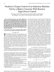
Fig. 1 illustrates the schematic diagram of PTC of IM drive. The torque reference is generated from the outer speed control loop via a proportional integral (PI) controller. Flux reference is generated based on the region of operation, constant torque, or field weakening (not considered in this work). The machine model is used for predicting the future torque and flux based on the measured and estimated states. Finally, an optimization step utilizes the reference and predicted quantities to generate the optimal gating signal for the next control sample which will be applied to 2L-VSI. In this section, the mathematical models required for the estimation and prediction steps will be explained along with the optimization step for the conventional method. A. Induction motor model The dynamic model of IM can be expressed using different representations depending on the reference frame used [24]. If the stator reference frame is adopted and the direct and quadrature components of stator current 𝑖 and rotor flux 𝜓 are considered as the state variables, the dynamic equations can be expressed as follows [18]. 𝑥 𝐴𝑥 𝐵𝑢 (1) 0 𝜔⎤ ⎡ 0 ⎤ ⎡ ⎢ ⎥ 0 𝜔 ⎢ 0 ⎥ ⎢ ⎥ 𝐴 ⎢ ⎥ (2) ⎥,𝐵 ⎢ 0 𝜔 ⎥ ⎢ ⎢ 0 0 ⎥ ⎢ ⎥ ⎣ 0 0 ⎦ 𝜔 ⎣0 ⎦ where 𝑥 𝑖 𝑖 𝜓 𝜓 are the state variables, 𝑢 𝑢 𝑢 is the stator voltage components, and 𝑅 and 𝑅 are stator and rotor resistances, 𝐿 , 𝐿 and 𝐿 are stator inductance, rotor inductance and mutual inductance respectively. 𝜔 is electrical rotor speed. 𝑘 is the rotor coupling factor. 𝑅

𝑅

𝑘 𝑅 represents the equivalent

𝐿 1

resistance. 𝐿

is the transient inductance of the

is the rotor time constant. 𝜏

machine. 𝜏

is the

stator transient time constant. The electromagnetic torque can be calculated as: 𝑇

𝑛

𝜓

𝑖

(3)

where 𝑛 is the number of pole pairs. The prediction step in MPC requires the knowledge of the discrete model of IM. Several discretization methods are available in literature [25]. For the sake of simplicity, Euler discretization method is used. The discrete state space model can be expressed using

Fig. 1. Schematic diagram of PTC of IM drive

𝑆 𝑆 𝑆

𝑉 0 0 0

𝑉 1 0 0

TABLE I SWITCHING STATES OF 2L- VSI 𝑉 𝑉 𝑉 𝑉 1 0 0 0 1 1 1 0 0 0 1 1

𝑉 1 0 1

𝑉 1 1 1


𝐴 𝑥

𝑥 𝛪

𝐴

𝑇𝐴,

𝐵 𝑢 𝐵

(4) 𝑇𝐵

(5)

where 𝛪 is the identity matrix and 𝑇 is the sampling time. B. Inverter model The two-level voltage source inverter has two switches per phase. Therefore, for three phases there are eight possible combinations of switching states 𝑆 resulting in eight voltage vectors as given in Table I. The applied stator voltage can be calculated as 𝑢

𝑢

𝑉 𝑇 𝑆

(6)

where 𝑉 is the DC link voltage, 𝑆 is the switching state and 𝑇 represents Clarke transformation. √

0

𝑇

√

(7)

1

C. Rotor flux estimation The rotor flux can be estimated from the rotor dynamics expressed at the rotor reference frame as follows. 𝜓

𝜏

𝐿 𝑖

(8)

Then, after using Euler discretization, it can be expressed as 𝜓

𝜓

𝑖

(9)

D. Prediction Knowing the rotor flux and using current measurement, Eq. (4) can be used to predict rotor flux one-step ahead. Then stator flux can be calculated at the 𝑘 1 sample from: 𝜓

𝑘 𝜓

𝐿 𝑖

(10)

It should be noted that the variables in (4) and (10) are expressed in stator reference frame. Therefore, appropriate coordinate transformation should be considered. In order to compensate for the time delay caused by calculation process, the variables at sample 𝑘 2 can be calculated as follow. 𝑥

𝐴 𝑥

𝐵 𝑢

(11)

𝜓

𝑘 𝜓

𝐿 𝑖

(12)

𝑇

𝑛

𝑉

𝜓

𝑖

𝑎𝑟𝑔 min 𝑔 𝑉

(13) (14)

E. Conventional optimization In this step, a predefined cost function 𝑔 is evaluated for all the possible voltage vectors. Then, the minimum value is determined and its corresponding voltage vector should be applied for the next sample period as follows. For PTC, the main objectives are to minimize torque and flux errors. The most common approach is to use the weighted sum of torque and flux errors as follows. 𝐾

𝑔 where 𝑇

and 𝜓

respectively. 𝑇 and ‖𝜓‖ are the rated torque and rated stator flux magnitude, respectively. 𝐾 is the flux weighting factor, which determines the relative importance of flux error. During the design process, 𝐾 should be carefully tuned in order to obtain good performance. One way to accomplish this is to consider a figure of merit like root mean square (RMS) errors of torque and flux and select a weighting factor compromising both [7]. Nevertheless, this task found to be tedious, since it has to be repeated if the operating point changes. Moreover, the 2L-VSI has seven different VVs. Therefore, the prediction and cost function calculation have to be repeated seven times in order to specify the optimal VV assuming one step prediction horizon is adopted. It becomes even worse and computationally more expensive if more complicated converter or longer prediction horizon are used.

‖

‖

(15)

are the torque and stator flux references,

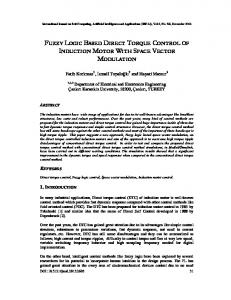
III. PROPOSED METHOD In this section, the superiority of the proposed method over the conventional one is discussed in terms of reducing the computational burden and setting the weighting factor. A. Reducing the computation burden The 2L-VSI has seven different VVs to be evaluated in the conventional method. In the proposed method, a group of four VVs, 𝑉 , will be evaluated each control sample and the optimal one will be selected. As a result, the computation burden of the prediction and optimization steps is reduced substantially. The group 𝑉 is updated each control sample based on the previous optimal VV and a predefined lookup table. Unlike [10], the proposed method is designed with two goals; reducing the switching frequency and maintaining good performance in terms of torque and flux ripples. Fig. 2 demonstrates the optimal VVs selected in the conventional method. From Fig. 2 (a), it can be noted that there is a pattern where nonzero VVs are changing in a certain sequence. For example, the optimal VV changes between 𝑉 and 𝑉 in a period followed by that where 𝑉 or 𝑉 are always selected as the optimal VV and so on. Moreover, this pattern repeats each electric cycle. In case, the zero voltage is selected to be the optimal VV, either 𝑉 or 𝑉 are selected based on reducing number of switches jump criterion. Final observation is illustrated in Fig. 2 (b) which represents a zoomed view for the period highlighted in Fig. 2 (a). If the previous VV was one of the zero VVs, there are two possibilities for the next optimal VV; either it returns to the last nonzero VV (𝑉 ) or returns to a VV adjacent to 𝑉 . These two cases are pointed at in Fig. 2 (b) by arrows. Based on the previous observations, the proposed method forms the candidate group 𝑉 based on the optimal VV of the previous sample 𝑉 . If the previous VV is nonzero, 𝑉 will be used directly to select the candidate group. On the other hand, if 𝑉 is one of the zero VVs, 𝑉 will be selected based on 𝑉 . Table II illustrates the voltage group formation based or 𝑉 . After the candidate group 𝑉 is on either 𝑉 determined, the cost function will be evaluated for each of the four VVs included. This method will also result in reducing the average switching frequency since the VVs in the candidate group are different from the old VV by only one


(a)

(b) Fig. 2 Simulation of Switching vector selection for the conventional method at rated speed without load (a) Complete electrical cycle (b) Zoomed view V3

V2

V4

V0

V1

V7

Fig. 4 Flowchart of the proposed method V5 V6

Fig. 3 Candidate voltage group in case that of 𝑉

𝑉

TABLE II VOLTAGE GROUP SELECTION 𝑉 OR 𝑉 𝑉 [𝑉 𝑉 𝑉 𝑉 ] 𝑉 [𝑉 𝑉 𝑉 𝑉 ] 𝑉 [𝑉 𝑉 𝑉 𝑉 ] [𝑉 𝑉 𝑉 𝑉 ] 𝑉 [𝑉 𝑉 𝑉 𝑉 ] 𝑉 [𝑉 𝑉 𝑉 𝑉 ] 𝑉

𝑔 𝑉

As discussed earlier, the design of the cost function and in particularly the flux weighting factor is not a trivial task as it greatly affects the overall performance of the motor [7], [13]. This will be even more obvious with the reduced number of voltage vectors. In order to avoid this complexity, eliminating the flux-weighting factor by relating the torque reference to the stator flux reference is adopted as follows [26]:

𝜓

𝑛 𝜆𝐿

𝜓

𝜓

(16)

𝑛 𝜆𝐿

𝜓

𝜓

(17)

𝜓

. exp 𝑗∠𝜓

(19)

A new cost function is formed that represents the deviation between the reference and predicted stator flux vectors.

B. Cost function design

𝑇

arcsin

where 𝜆

switch state as indicated in Tables I and II. Fig. 3 illustrates an example of the candidate VV group in case of 𝑉 is 𝑉 . In this case 𝑉 is {𝑉 , 𝑉 , 𝑉 , 𝑉 } from which the optimal VV will be selected based on the used cost function.

𝑇

∠𝜓

∠𝜓

is 𝑉

(18)

𝜓

𝜓

(20)

Since the new cost function contains only stator flux, no weighting factors are required. This greatly simplify the design process by avoiding online tuning necessary for the conventional method. The value of stator flux at step 𝑘 2 can be calculated as follows: 𝜓

𝜓

𝑇 𝑉

𝑅 𝑖

(21)

represents one of the candidate VV. The last step where 𝑉 is to select the VV that minimizes the cost function among the candidate group 𝑉 as follows: 𝑉

arg min 𝑔 𝑉

(22)

The main steps of the proposed algorithm is illustrated in the flowchart of Fig. 4. For the sake of comparison, the performance of the proposed method will be assessed in the following sections versus the conventional method and the reduced switching frequency (RSF) method reported in [10]. The latter aims to reduce the average switching frequency by limiting the


T (N.m)

r

(rpm)

selection of the optimal voltage vector to those with minimum number of switching jumps. In this case, the cost function in (17) is repeated only four times based on a preselected four VVs. These VVs are updated each control sample based on the previous optimal VV such that at most one of the three states 𝑆 , 𝑆 , 𝑆 is allowed to change. For example if the previous optimal VV is (1,0,0), the four allowable VVs are (1,0,0), (1,1,0), (1,0,1), (0,0,0). This method leads to reduction in the computation burden and the average switching frequency. On the other hand, the torque and flux ripples deteriorate compared to the conventional method [10].

Parameter 𝑃 𝑁 𝑅 𝐿 𝐿 𝐽

TABLE III INDUCTION MOTOR PARAMETERS Value Parameter 1 Kw 𝑇 ‖𝜓 ‖ 1710 rpm 8.15 Ω Rr 0.4577 H Lr 𝑛 0.4372 H 0.007 Kg.m2 B

TABLE IV CONTROLLER PARAMETERS Description Symbol Simulation time 𝑇 PTC Sampling time 𝑇 𝐾 Flux weighting factor 𝐾 Proportional gain Integral gain 𝐾

Value 5.58 N.m 0.8157 Wb 6.0373 Ω 0.4577 H 2 0 N.m.s

Value 2.5 µsec 40 µsec 8 0.63 14.17

ia (A)

s

(wb)

IV. SIMULATION RESULTS

ia (A)

s

(wb)

T (N.m)

r

(rpm)

(a)

(b)

The proposed method is simulated using MATLAB Simulink. For the sake of comparison, the reduced switching frequency (RSF) [10] with one step prediction and the conventional method (17) are also simulated using the same flux weighting factor which have been selected based on offline simulation trial [7]. The machine parameters used in the simulation are listed in Table III while the designed controller parameters are given in Table IV. Firstly, the flux is built to its rated value then the speed command is applied at 𝑡 0.1 sec. This pre-excitation process helps in reducing the starting current [27]. Finally, at 𝑡 0.5 sec, rated load is applied. The same PI controller gains for the outer speed loop is used for all the methods. Fig. 5 illustrates the dynamic response of the IM drive system for all methods where speed, torque, flux and phase current are illustrated from up to bottom respectively. The responses of Fig. 5 indicate that the proposed method has fast dynamic response and robustness against external load disturbance. It can also be noted that from the viewpoint of dynamics, the responses of all the methods are comparable. In order to test the robustness of the proposed method against parameter variation, system response is studied under varying both stator and rotor resistances. Fig. 6 illustrates their effect on the performance on the drive system at rated load and at both rated and low speed operating conditions. It can be seen that the system response is satisfactory under the variation up to 129% and 117% at rated speed and very low speed, respectively. V. EXPERIMENTAL RESULTS A. Hardware description

(c) Fig. 5 Simulated starting and loading response (a) Conventional (b) RSF (c) Proposed methods

Fig. 7 illustrates the experimental setup used. A 1.0 kW induction motor with the same parameters as in the simulation study is used. A 0.75 kW separately excited DC generator is mechanically coupled to the motor. The terminal of the DC generator is connected to a programmable electronic load. The motor is fed by a controlled 2L-VSI from SEMKRON. The PTC algorithm is implemented in real time using dSPACE 1103 (1 GHz) platform. The sample time for all the algorithms is set to 40 𝜇sec. The speed is measured using a 1024 pulse


2000 1800 1600 0.9

1

1.1

1.2

1.3

1.4

1.5

1.6

1.7

1.8

1

1.1

1.2

1.3

1.4

1.5

1.6

1.7

1.8

1

1.1

1.2

1.3

1.4

1.5

1.6

1.7

1.8

1

1.1

1.2

1.3

1.4

1.5

1.6

1.7

1.8

10 5 0 0.9 1 0.5 0 0.9 100 75 50 25 0 0.9

Time (sec)

(rpm)

(a)

Fig. 8 Experimental Dynamic torque response for conventional and proposed methods

r

100

0 0.9

1

1.1

1.2

1.3

1.4

1.5

1.6

1.7

1.8

1

1.1

1.2

1.3

1.4

1.5

1.6

1.7

1.8

1

1.1

1.2

1.3

1.4

1.5

1.6

1.7

1.8

1

1.1

1.2

1.3

1.4

1.5

1.6

1.7

1.8

T (N.m)

50

10

0 0.9

s

1

(wb)

5

0 0.9 100 75

ia (A)

0.5

50 25 0 0.9

(a)

r

ia (A)

s

(wb)

T (N.m)

(b) Fig. 6 robustness test of the proposed method under rated load and (a) rated speed (b) low speed of 50 rpm

(rpm)

Time (sec)

(b) Fig. 9 Experimental starting response from zero to rated speed at noload using (a) Conventional (b) Proposed methods

Fig. 7 Experimental setup (a) Semikron Inverter (b) LEM Sensors (c) 15V dc supply (d) dSPACE terminal box (e) Host PC (f) Chroma programmable load (g) DC generator (h) Incremental encoder (i) Induction motor

per revolution incremental encoder and a low pass filter is adopted to reduce the quantization error. In order to demonstrate torque dynamic characteristics, a step change in the speed command from 1000 to 1400 rpm is

applied. This results in saturating the PI controller and causing the torque command to step to its maximum value. Fig. 8 illustrates the dynamics of the electromagnetic torque for both conventional and proposed methods. It can be seen that the dynamic torque response with the proposed method does not degrade compared to conventional method where they reach the new reference in less than one msec. B. Dynamic characteristics Fig. 9 shows the starting from the standstill to the rated speed of the machine. The same pre-excitation process depicted in the simulation section is used. Both the


ia (A)

s

(wb)

T (N.m)

r

(rpm)

conventional method and the proposed method has similar starting responses as shown in Fig. 9 decoupled control of torque and flux is achieved in the proposed method. Therefore, the same performance of the conventional method is maintained with simpler design of the cost function due to elimination of flux weighting factor.

(a)

(b) Fig. 10 Experimental sudden load response at rated speed and rated load using (a) Conventional (b) Proposed methods 4000 3000 2000 1000 0 8

Reference Measured

0

0.2

0.4

0.6

0.8

1

1.2 T

4

1.4

1.6 T

ref

est

In order to test the robustness against external load, the rated load is applied to the motor while running at rated speed. Fig. 10 shows the sudden loading response for the conventional and the proposed method. The proposed method successfully regains its reference speed after a short transient period in a manner similar to the conventional method proving its robustness against load disturbance. The performance of the proposed method at very high speed is investigated. Fig. 11 illustrates the response of the proposed method in the field weakening region. The motor is commanded to start from standstill to 3600 rpm. Up to the base speed the flux is set to its rated value. For speed higher than base speed, the flux command is varied inversely to the rotor speed and the maximum torque is varied in proportion to square of the reference flux [28]. By examining the torque and flux responses, it can be noted that both of them track their references perfectly even in the field weakening region when both flux and torque references are varying simultaneously. Moreover, the response of the proposed algorithm under maximum torque per ampere (MTPA) criteria is also investigated. MTPA method based on using lookup table (LUT) to generate reference stator flux based on torque reference is adopted [29]. Knowing torque and flux references the proposed PTC method can be used as illustrated in Fig. 1. The relation between stator flux and torque under the utilized MTPA method is illustrated in Fig. 12. It can be noted from Fig. 12 that the minimum value of the flux is set to 0.1 Wb at zero torque to avoid excessive flux reduction. Moreover, due to limitation of direct axis current [29], the value of the flux saturates at its rated value. In order to apply step torque command, the reference speed is changed from 300 to 500 rpm with a load of 2 NM. This will saturate the outer speed controller and the reference torque will reach its maximum value. The operating speeds have been selected such that the operation will be in flux increase region and there will be feasible voltage vector capable of tracking torque and flux references [30]. Experimental results illustrating this test is shown in Fig. 13. For MTPA, the flux and torque are related as illustrated in Fig. 12. As a result, a step in the flux reference is evident. It can be clearly noted that both the flux and torque tracks perfectly their references with very fast dynamics. Moreover, it is clear that the current response is limited. Even though there is no direct limitation on the current in the proposed method, the current will be bounded due to the limitation on the machine torque and flux. The variation of the load angle is

0 1 0.8

0

0.2

0.4

0.6

0.8

1

1.2

1.4 ref

1.6 est

0.4 0 5

0

0.2

0.4

0.6

0.8

1

1.2

1.4

1.6

0

0.2

0.4

0.6

0.8

1

1.2

1.4

1.6

0 -5

Time (sec) Fig. 11 Experimental starting response from zero to 3600 rpm at noload using the proposed methods

Fig. 12 Visualization of LUT used for flux reference calculation under MTPA criteria


(a) Fig. 13 Experimental MTPA operation using the proposed method

illustrated at the very bottom curve of Fig. 13. It is clear that the load angle is less than 45 which guarantees stable operation and that the maximum slip will not be exceeded. Finally, a speed reversal test is implemented. Fig. 14 (a) to (c) demonstrates the speed reversal from 1710 to -1710 rpm at no-load condition for the conventional, RSF, and the proposed method, respectively. For the proposed and conventional methods, it can be noted that the flux is fixed to its rated value during all the transient period proving the decoupled effect between flux and torque control. On the other hand, the flux ripple, torque ripple, and current distortion increase significantly with the RSF method. Similar response was reported in [10] for the RSF method. This indicates that the RSF cannot work properly at low speed high torque operating point where further tuning for the flux-weighting factor is required. The torque response for the proposed method is uniform. This is due to the WFE method utilized in the proposed approach, which automatically compromise between torque and flux errors in contrast to the fixed flux-weighting factor used for both RSF and the conventional method.

(b)

C. Steady state analysis For further comparison among the three methods, deeper steady state analysis is presented. Fig. 15 illustrates the low speed operation at 50 rpm and no-load condition. It can clearly be noticed that the RSF has the worst response with the highest torque ripple and most distorted current waveform. The proposed method has lower torque and flux ripple than the conventional method. In addition, the current waveform is uniform and sinusoidal unlike the distorted waveform, which can be observed in the RSF method current waveform. In order to cover different operating points, the response of the three methods have been recorded at different speed and (2.5 Nm) load. Torque ripple, flux ripple, current THD, and average switching frequency are calculated and the results are listed in Table V. Analysis of the third column in Table V clearly indicate that the proposed method is superior regarding the torque ripple for all the speed range. On the other hand, the RSF method has the highest torque ripple. The flux ripple of the proposed method is comparable to the conventional method and shows a slight increase at some operating speed.

(c) Fig. 14 Experimental speed reversal at 1710 rpm and no-load condition (a) Conventional (b) RSF (c) Proposed methods

It is still much lower than the flux ripple measured for RSF method. As expected form the design of the proposed and RSF methods, both of them have lower average switching frequency compared to the conventional method as can be observed from the measured average switching frequency in Table V. Although there is a little increase in the average switching frequency of the proposed method, the reduction of the torque and flux ripples is quite evident. The current THD for the three methods is shown in the last column in Table V. It can be noted that proposed method has a little higher THD values compared to the conventional method. This can be expected due to the reduced average


T (N.m)

1 0 -1 0

0.1

0.2

0.3

0.4

0.5

0.6

0.7

0.8

0.9

1

0

0.1

0.2

0.3

0.4

0.5

0.6

0.7

0.8

0.9

1

0

0.1

0.2

0.3

0.4

0.5

0.6

0.7

0.8

0.9

1

(wb)

0.84

s

0.82 0.8 0.78

ia (A)

2 0 -2

Time (sec)

TABLE V PERFORMANCE COMPARISON AMONG THREE PTC METHODS AT 2.5 NM

(a) 1

T (N.m)

and optimization steps. The RSF method has the shortest execution time since it need to repeat the prediction and optimization steps four times only. Although the proposed method need also four iteration for prediction and optimization, it has longer execution time compared to the RSF method. This is due to the time required for reference flux vector calculation, which is necessary for eliminating the need for flux weighting factor. Even though the execution time is still less than that of the conventional method as indicated in Table VI. Actually, about 18 % reduction in the execution time can be achieved using the proposed method compared to the conventional one. The results of Table V and VI show clearly the efficiency of the proposed method and its ability to compromise among different figure of merits.

𝑁 𝑟𝑝𝑚

0

300

-1 0

0.1

0.2

0.3

0.4

0.5

0.6

0.7

0.8

0.9

1

(wb)

0.84

600

s

0.82 0.8 0.78

0

0.1

0.2

0.3

0.4

0.5

0.6

0.7

0.8

0.9

1

1000

ia (A)

2

1400

0 -2 0

0.1

0.2

0.3

0.4

0.5

0.6

0.7

0.8

0.9

1

Time (sec)

(b) T (N.m)

1

0

0.1

0.2

0.3

0.4

0.5

0.6

0.7

0.8

0.9

1

0.84

(wb)

Conv RSF Proposed Conv RSF Proposed Conv RSF Proposed Conv RSF Proposed Conv RSF Proposed

𝑇

𝑁𝑚

0.813 0.895 0.761 0.718 0.789 0.621 0.807 0.775 0.646 0.724 0.711 0.573 0.703 0.665 0.618

𝜓

𝑤𝑏

0.012 0.019 0.014 0.012 0.017 0.015 0.012 0.018 0.013 0.012 0.014 0.013 0.013 0.012 0.011

𝑓

𝐾𝐻𝑧 4.24 2.31 2.53 5.50 2.89 4.13 5.11 3.52 4.44 3.76 3.34 3.49 2.67 2.66 2.54

𝑖

% 6.93 9.69 7.26 6.36 9.91 6.99 6.15 10.38 6.64 6.42 8.59 6.63 7.21 7.21 6.95

TABLE VI COMPUTATION TIMES FOR DIFFERENT PTC METHODS

0 -1

s

1710

Method

Method Conventional RSF Proposed

Pred &opt 𝜇sec 1.9 1.23 1.56

Total 𝜇sec 10.3 9.51 9.87

0.82 0.8 0.78

VI. CONCLUSION 0

0.1

0.2

0.3

0.4

0.5

0.6

0.7

0.8

0.9

1

0

0.1

0.2

0.3

0.4

0.5

0.6

0.7

0.8

0.9

1

ia (A)

2 0 -2

Time (sec)

(c) Fig. 15 Low speed response at 50 rpm and no-load condition (a) Conventional (b) RSF (c) Proposed methods

switching frequency of the proposed method. In addition, the RSF method has the worst current THD since its deteriorated flux response is reflected on the current waveform. Finally, the average execution time of the three method is recorded in Table VI. Since the methods differ only in the prediction and optimization steps, only the sum of prediction and optimization steps and total execution times are reported. The conventional method has the longest execution time as expected with seven iteration required to finish the prediction

This paper presents a simple and efficient PTC algorithm for IM drives. The proposed method has two salient features over the conventional method, reduced computational cost and elimination of flux weighting factor. The latter not only simplifies the design process of the algorithm but also guarantees an optimized performance. Simulation and experimental results shows clearly the superiority of the proposed method at different operating conditions. Compared to the conventional method, the proposed one has lower torque ripple and average switching frequency. Flux ripple and current THD of the proposed method is comparable to the conventional method. Moreover, the proposed approach is compared to RSF method reported in literature. The proposed one shows an enhanced performance compared to the RSF method, which is reflected on reduction in torque and flux ripples and current THD. Even with the added online computation required for avoiding offline design of fluxweighting factor, the proposed method still has shorter execution time compared to the conventional method.


REFERENCES [1] [2] [3] [4]

[5]

[6] [7]

[8] [9] [10]

[11] [12] [13]

[14]

[15]

[16]

[17] [18] [19]

[20]

[21]

J. H. Lee, “Model predictive control: Review of the three decades of development,” Int. J. Control. Autom. Syst., vol. 9, no. 3, pp. 415–424, 2011. C. E. García, D. M. Prett, and M. Morari, “Model predictive control: Theory and practice—A survey,” Automatica, vol. 25, no. 3, pp. 335– 348, 1989. A. Linder and R. Kennel, “Model Predictive Control for Electrical Drives,” Power Electron. Spec. Conf. 2005. PESC ’05. IEEE 36th, pp. 1793–1799, 2005. J. Rodriguez, M. P. Kazmierkowski, J. R. Espinoza, P. Zanchetta, H. Abu-Rub, H. A. Young, and C. A. Rojas, “State of the Art of Finite Control Set Model Predictive Control in Power Electronics,” IEEE Trans. Ind. Informatics, vol. 9, no. 2, pp. 1003–1016, 2013. S. Vazquez, J. Rodriguez, M. Rivera, L. G. Franquelo, and M. Norambuena, “Model Predictive Control for Power Converters and Drives: Advances and Trends,” IEEE Trans. Ind. Electron., vol. 64, no. 2, pp. 935–947, 2017. F. Wang, X. Mei, J. Rodriguez, and R. Kennel, “Model Predictive Control for Electrical Drive Systems-An Overview,” Ces Trans. Electr. Mach. Syst., vol. 1, no. 3, pp. 219–230, 2017. P. Cortes, S. Kouro, B. La Rocca, R. Vargas, J. Rodriguez, J. I. Leon, S. Vazquez, and L. G. Franquelo, “Guidelines for weighting factors design in Model Predictive Control of power converters and drives,” IEEE Int. Conf. Ind. Technol., pp. 1–7, 2009. T. Geyer, “Computationally efficient model predictive direct torque control,” IEEE Trans. Power Electron., vol. 26, no. 10, pp. 2804–2816, 2011. T. Geyer and D. E. Quevedo, “Multistep finite control set model predictive control for power electronics,” IEEE Trans. Power Electron., vol. 29, no. 12, pp. 6836–6846, 2014. F. Wang, Z. Zhang, A. Davari, J. Rodríguez, and R. Kennel, “An experimental assessment of finite-state Predictive Torque Control for electrical drives by considering different online-optimization methods,” Control Eng. Pract., vol. 31, pp. 1–8, 2014. M. Habibullah, D. D.-C. Lu, D. Xiao, and M. F. Rahman, “A Simplified Finite-State Predictive Direct Torque Control for Induction Motor Drive,” IEEE Trans. Ind. Electron., vol. 63, no. 6, pp. 3964–3975, 2016. C. Xia, S. Member, T. Liu, T. Shi, and Z. Song, “A Simplified FiniteControl-Set Model-Predictive Control for Power Converters,” IEEE Trans. Ind. Informatics, vol. 10, no. 2, pp. 991–1002, 2014. S. A. Davari, D. A. Khaburi, and R. Kennel, “An improved FCS-MPC algorithm for an induction motor with an imposed optimized weighting factor,” IEEE Trans. Power Electron., vol. 27, no. 3, pp. 1540–1551, 2012. P. Zanchetta, “Heuristic Multi-Objective Optimization for Cost Function Weights Selection in Finite States Model Predictive Control,” 2011 IEEE Work. Predict. Control Electr. Drives Power Electron., pp. 70–75, 2011. F. Villarroel, J. R. Espinoza, C. A. Rojas, J. Rodriguez, M. Rivera, and D. Sbarbaro, “Multiobjective Switching State Selector for Finite-States Model Predictive Control Based on Fuzzy Decision Making in a Matrix Converter,” IEEE Trans. Ind. Electron., vol. 60, no. 2, pp. 589–599, 2013. A. A. Ahmed, B.-K. Koh, H. S. Park, K.-B. Lee, and Y. Il Lee, “Finite Control Set Model Predictive Control Method for Torque Control of Induction Motors using a State Tracking Cost Index,” IEEE Trans. Ind. Electron., vol. 46, no. c, pp. 1–1, 2016. C. A. Rojas, J. Rodriguez, F. Villarroel, J. R. Espinoza, C. A. Silva, and M. Trincado, “Predictive Torque and Flux Control Without Weighting Factors,” IEEE Trans. Ind. Electron., vol. 60, no. 2, pp. 681–690, 2013. C. A. Rojas and J. Rodriguez, “Multiobjective Fuzzy-Decision-Making Predictive Torque Control for an InductionMotor Drive,” IEEE Trans. Power Electron., vol. 32, no. 8, pp. 6245–6260, 2017. M. Mamdouh, A. Salem, and M. A. Abido, “An improved multiobjective fuzzy decision based predictive torque control of induction motor drive,” in IECON 2017 - 43rd Annual Conference of the IEEE Industrial Electronics Society, 2017, pp. 8675–8680. V. P. Muddineni, A. K. Bonala, and S. R. Sandepudi, “Enhanced weighting factor selection for predictive torque control of induction motor drive based on VIKOR method,” IET Electr. Power Appl., vol. 10, no. 9, pp. 877–888, 2016. V. P. Muddineni, S. R. Sandepudi, and A. K. Bonala, “Finite control set predictive torque control for induction motor drive with simplified

[22] [23]

[24] [25]

[26]

[27] [28] [29]

[30]

weighting factor selection using TOPSIS method,” IET Electr. Power Appl., vol. 11, no. 5, pp. 749–760, 2017. Y. Zhang and H. Yang, “Model-Predictive Flux Control of Induction Motor Drives With Switching Instant Optimization,” IEEE Trans. Energy Convers., vol. 30, no. 3, pp. 1113–1122, 2015. M. Mamdouh, M. A. Abido, and Z. Hamouz, “Weighting Factor Selection Techniques for Predictive Torque Control of Induction Motor Drives: A Comparison Study,” Arab. J. Sci. Eng., vol. 43, no. 2, pp. 433–445, Feb. 2018. J. Holtz, “The dynamic representation of AC drive systems by complex signal flow graphs,” Proc. 1994 IEEE Int. Symp. Ind. Electron., pp. 1–6, 1994. C. A. Rojas, J. I. Yuz, M. Aguirre, and J. Rodriguez, “A comparison of discrete-time models for model predictive control of induction motor drives,” in 2015 IEEE International Conference on Industrial Technology (ICIT), 2015, pp. 568–573. Y. Zhang and H. Yang, “Model predictive control of induction motor drives: Flux control versus torque control,” in 2015 9th International Conference on Power Electronics and ECCE Asia (ICPE-ECCE Asia), 2015. Y. Zhang, J. Zhu, Z. Zhao, W. Xu, and D. G. Dorrell, “An Improved Direct Torque Control for Three-Level Sensorless drive,” IEEE Trans. Power Electron., vol. 27, no. 3, pp. 1502–1513, 2012. D. Casadei, G. Serra, A. Stefani, A. Tani, and L. Zarri, “DTC drives for wide speed range applications using a robust flux-weakening algorithm,” IEEE Trans. Ind. Electron., vol. 54, no. 5, pp. 2451–2461, 2007. R. Bojoi, Z. Li, S. A. Odhano, G. Griva, and A. Tenconi, “Unified direct-flux vector control of induction motor drives with maximum torque per ampere operation,” in 2013 IEEE Energy Conversion Congress and Exposition, ECCE 2013, 2013, pp. 3888–3895. A. A. Ahmed, B. K. Koh, H. S. Park, K.-B. Lee, and Y. Il Lee, “FiniteControl Set Model Predictive Control Method for Torque Control of Induction Motors Using a State Tracking Cost Index,” IEEE Trans. Ind. Electron., vol. 64, no. 3, pp. 1916–1928, 2017.

M. Mamdouh (S’16) was born in Kafer El-Zayat, Gharbia, Egypt in 1985. He received his B.Sc. (Honors with first class) in electrical power and machines, Faculty of Engineering, Tanta University, Egypt in 2007. He received his M.Sc. in mechatronics and robotics from Egypt-Japan University of Science and Technology (E-JUST), Egypt in 2012. He received his Ph.D. in electrical engineering from King Fahd University of Petroleum and Minerals (KFUPM) in 2018. He currently works as assistant professor at Electrical Power and Machines Department, Faculty of Engineering, Tanta University, Egypt. His current research interest is model predictive control of electric drive systems. M. A. Abido (SM’15) received the B.Sc. (Honors with first class) and M.Sc. degrees in EE from Menoufia University, Shebin El-Kom, Egypt, in 1985 and 1989, respectively, and the Ph.D. degree from King Fahd University of Petroleum and Minerals (KFUPM), Dhahran, Saudi Arabia, in 1997. He is currently a Distinguished University Professor at KFUPM. His research interests are power system stability, planning, operation, and optimization techniques applied to power systems. Dr. Abido is the recipient of KFUPM Excellence in Research Award, 2002, 2007 and 2012, KFUPM Best Project Award, 2007 and 2010, First Prize Paper Award of the Industrial Automation and Control Committee of the IEEE Industry Applications Society, 2003, Abdel-Hamid Shoman Prize for Young Arab Researchers in Engineering Sciences, 2005, Best Applied Research Award of 15th GCC-CIGRE Conference, Abu-Dhabi, UAE, 2006, and Best Poster Award, International Conference on Renewable Energies and Power Quality (ICREPQ’13), Bilbao, Spain, 2013. Dr. Abido has been awarded Almarai Prize for Scientific Innovation 20172018, Distinguished Scientist, Saudi Arabia, 2018 and Khalifa Award for Education 2017-2018, Higher Education, Distinguished University Professor in Scientific Research, Abu Dhabi, UAE, 2018. Dr. Abido has published two books and more than 350 papers in reputable journals and international conferences. He participated in 50+ funded projects and supervised 50+ MS and PhD students