then a query execution engine runtime is responsible for executing the query ..... ports my adaptive query optimization techniques, and I present a basic set of ...
Efficient Query Processing for Data Integration
Zachary G. Ives
A dissertation submitted in partial fulfillment of the requirements for the degree of
Doctor of Philosophy
University of Washington 2002
Program Authorized to Offer Degree: Department of Computer Science and Engineering
University of Washington Graduate School
This is to certify that I have examined this copy of a doctoral dissertation by Zachary G. Ives and have found that it is complete and satisfactory in all respects, and that any and all revisions required by the final examining committee have been made.
Chair of Supervisory Committee:
Alon Halevy
Reading Committee:
Alon Halevy (chair) Daniel Weld Dan Suciu
Date:
In presenting this dissertation in partial fulfillment of the requirements for the Doctoral degree at the University of Washington, I agree that the Library shall make its copies freely available for inspection. I further agree that extensive copying of this dissertation is allowable only for scholarly purposes, consistent with “fair use” as prescribed in the U.S. Copyright Law. Requests for copying or reproduction of this dissertation may be referred to Bell and Howell Information and Learning, 300 North Zeeb Road, Ann Arbor, MI 48106-1346, or to the author.
Signature
Date
University of Washington Abstract
Efficient Query Processing for Data Integration by Zachary G. Ives Chair of Supervisory Committee: Professor Alon Halevy Computer Science and Engineering
A major problem today is that important data is scattered throughout dozens of separately evolved data sources, in a form that makes the “big picture” difficult to obtain. Data integration presents a unified virtual view of all data within a domain, allowing the user to pose queries across the complete integrated schema. This dissertation addresses the performance needs of real-world business and scientific applications. Standard database techniques for answering queries are inappropriate for data integration, where data sources are autonomous, they generally lack mechanisms for sharing of statistical information about their content, and the environment is shared with other users and subject to unpredictable change. My thesis proposes the use of pipelined and adaptive techniques for processing data integration queries, and I present a unified architecture for adaptive query processing, including novel algorithms and an experimental evaluation. An operator called x-scan extracts the relevant content from an XML source as streams across the network, which enables more work to be done in parallel. Next, the query is answered using algorithms (such as an extended version of the pipelined hash join) whose work is adaptively scheduled, varying to accommodate the relative data arrival rates of the sources. Finally, the system can adapt the ordering of the various operations (the query plan), either at points where the data is being saved to disk or in mid-execution, using a novel technique called convergent query processing. I show that these techniques provide significant benefits in processing data integration queries.
TABLE OF CONTENTS
List of Figures
iii
List of Tables Chapter 1:
v Introduction
1
1.1 The Motivations for Data Integration
. . . . . . . . . . . . . . . . . . . .
2
1.2 Query Processing for Data Integration . . . . . . . . . . . . . . . . . . . .
5
1.3 Outline of Dissertation . . . . . . . . . . . . . . . . . . . . . . . . . . . . .
10
Chapter 2:
Background: Data Integration and XML
12
2.1 Data Integration System Architecture . . . . . . . . . . . . . . . . . . . .
12
2.2 The XML Format and Data Model . . . . . . . . . . . . . . . . . . . . . .
16
2.3 Querying XML Data . . . . . . . . . . . . . . . . . . . . . . . . . . . . . .
20
Chapter 3:
Query Processing for Data Integration
25
3.1 Position in the Space of Adaptive Query Processing . . . . . . . . . . . .
26
3.2 Adaptive Query Processing for Data Integration . . . . . . . . . . . . . .
28
3.3 The Tukwila Data Integration System: An Adaptive Query Processor . .
33
Chapter 4:
An Architecture for Pipelining XML Streams
36
4.1 Previous Approaches to XML Processing . . . . . . . . . . . . . . . . . . .
40
4.2 The Tukwila XML Architecture . . . . . . . . . . . . . . . . . . . . . . . .
42
4.3 Streaming XML Input Operators . . . . . . . . . . . . . . . . . . . . . . .
50
4.4 Tukwila XML Query Operators . . . . . . . . . . . . . . . . . . . . . . . .
58
4.5 Supporting Graph-Structured Data in Tukwila . . . . . . . . . . . . . . .
61
4.6 Experimental Results . . . . . . . . . . . . . . . . . . . . . . . . . . . . . .
66
4.7 Conclusions
81
. . . . . . . . . . . . . . . . . . . . . . . . . . . . . . . . . . . i
Chapter 5:
Execution Support for Adaptivity
83
5.1 An Adaptive Execution Architecture . . . . . . . . . . . . . . . . . . . . .
87
5.2 Adaptive Query Operators . . . . . . . . . . . . . . . . . . . . . . . . . . .
94
5.3 Experiments . . . . . . . . . . . . . . . . . . . . . . . . . . . . . . . . . . .
101
5.4 Conclusions
107
Chapter 6:
. . . . . . . . . . . . . . . . . . . . . . . . . . . . . . . . . . .
Adaptive Optimization of Queries
109
6.1 Convergent Query Processing . . . . . . . . . . . . . . . . . . . . . . . . .
113
6.2 Operators for Phased Execution . . . . . . . . . . . . . . . . . . . . . . . .
119
6.3 Implementation within Tukwila . . . . . . . . . . . . . . . . . . . . . . . .
122
6.4 Experiments . . . . . . . . . . . . . . . . . . . . . . . . . . . . . . . . . . .
127
6.5 Conclusion . . . . . . . . . . . . . . . . . . . . . . . . . . . . . . . . . . . .
135
Chapter 7:
Tukwila Applications and Extensions
137
7.1 Data Management for Ubiquitous Computing . . . . . . . . . . . . . . . .
137
7.2 Peer Data Management
. . . . . . . . . . . . . . . . . . . . . . . . . . . .
139
7.3 Integration for Medicine: GeneSeek . . . . . . . . . . . . . . . . . . . . .
142
7.4 Summary . . . . . . . . . . . . . . . . . . . . . . . . . . . . . . . . . . . . .
143
Chapter 8:
Related Work
145
8.1 Data Integration (Chapter 2) . . . . . . . . . . . . . . . . . . . . . . . . .
145
8.2 XML Processing (Chapter 4) . . . . . . . . . . . . . . . . . . . . . . . . . .
148
8.3 Adaptive Query Processing (Chapters 5, 6) . . . . . . . . . . . . . . . . .
152
Chapter 9:
Conclusions and Future Directions
158
9.1 Future Work in Adaptive Query Processing . . . . . . . . . . . . . . . . .
159
9.2 Envisioning a Universal Data Management Interface . . . . . . . . . . .
161
Bibliography
166
ii
LIST OF FIGURES
1.1 Data warehousing and integration compared . . . . . . . . . . . . . . . .
4
2.1 Data integration architecture diagram . . . . . . . . . . . . . . . . . . . .
13
2.2 Sample XML document . . . . . . . . . . . . . . . . . . . . . . . . . . . . .
17
2.3 XML-QL graph representation of example data . . . . . . . . . . . . . . .
18
2.4 XQuery representation of example data . . . . . . . . . . . . . . . . . . .
19
2.5 Example XQuery over sample data . . . . . . . . . . . . . . . . . . . . . .
21
2.6 Results of example query . . . . . . . . . . . . . . . . . . . . . . . . . . . .
22
3.1 Architecture diagram of Tukwila . . . . . . . . . . . . . . . . . . . . . . .
33
4.1 Tukwila XML query processing architecture
. . . . . . . . . . . . . . . .
44
4.2 Example XQuery to demonstrate query plan . . . . . . . . . . . . . . . .
46
4.3 Example Tukwila query plan . . . . . . . . . . . . . . . . . . . . . . . . .
47
4.4 Encoding of a tree within a tuple . . . . . . . . . . . . . . . . . . . . . . .
48
4.5 Basic operation of x-scan operator
. . . . . . . . . . . . . . . . . . . . . .
52
4.6 The web-join operator generalizes the dependent join . . . . . . . . . . .
57
4.7 X-scan components for processing graph-structured data . . . . . . . . .
63
4.8 Experimental evaluation of different XML processors . . . . . . . . . . .
69
4.9 Wide-area performance of query processors . . . . . . . . . . . . . . . . .
71
4.10 Comparison of data set sizes and running times . . . . . . . . . . . . . .
73
4.11 Scale-up of x-scan for simple and complex paths . . . . . . . . . . . . . .
74
4.12 Experimental comparison of XML vs. JDBC as a transport . . . . . . . .
77
4.13 Comparison of nest and join operations . . . . . . . . . . . . . . . . . . .
78
4.14 Scale-up results for x-scan over graph and tree-based data . . . . . . . .
80
4.15 Query processing times with bounded memory . . . . . . . . . . . . . . .
80
5.1 Example of query re-optimization . . . . . . . . . . . . . . . . . . . . . . .
86
5.2 Example of collector policy rules
95
. . . . . . . . . . . . . . . . . . . . . . . iii
5.3 Performance benefits of pipelined hash join . . . . . . . . . . . . . . . . .
103
5.4 Comparison of Symmetric Flush vs. Left Flush overflow resolution . . .
105
5.5 Interleaved planning and execution produces overall benefits
. . . . . .
106
6.1 Example of phased query execution for 3-way join . . . . . . . . . . . . .
115
6.2 Architecture of the Tukwila convergent query processor . . . . . . . . . .
123
6.3 Experimental results over 100Mbps LAN . . . . . . . . . . . . . . . . . .
129
6.4 Experimental results over slow network . . . . . . . . . . . . . . . . . . .
132
6.5 Performance of approach under limited memory . . . . . . . . . . . . . .
133
7.1 Example of schema mediation in a PDMS . . . . . . . . . . . . . . . . . .
140
7.2 Piazza system architecture . . . . . . . . . . . . . . . . . . . . . . . . . . .
141
iv
LIST OF TABLES
4.1 Physical query operators and algorithms in Tukwila . . . . . . . . . . . .
59
4.2 Experimental data sets . . . . . . . . . . . . . . . . . . . . . . . . . . . . .
67
4.3 Systems compared in Section 4.6.1. . . . . . . . . . . . . . . . . . . . . . .
68
4.4 List of pattern-matching queries . . . . . . . . . . . . . . . . . . . . . . .
68
4.5 List of queries used in XML processing experiments . . . . . . . . . . . .
75
6.1 Data sources for experiments . . . . . . . . . . . . . . . . . . . . . . . . .
128
8.1 Comparison of adaptive query processing techniques . . . . . . . . . . .
157
v
ACKNOWLEDGMENTS
Portions of this dissertation have previously been published in SIGMOD [IFF+ 99] and in the IEEE Data Engineering Bulletin [IHW01, ILW+ 00]. However, these portions have been significantly revised and extended within this dissertation. Additionally, portions of Chapter 4 have been submitted concurrently to the VLDB Journal. It’s amazing to look back and see how things have changed over the past few years, how others have influenced me. I’ve been blessed with a brilliant and incredibly generous group of collaborators and advisors, who’ve given me great ideas and shaped my research ideas and my thesis work. Special thanks to my advisors, Alon Halevy and Dan Weld, who let me be creative but kept me on track, and with whom I’ve had countless stimulating discussions that led to new ideas. Even more importantly, they taught me choose worthwhile problems and aim high. I have come to understand just how critical this is in the research world. Thanks also to Steve Gribble, Hank Levy, and Dan Suciu for showing me a broader perspective on my research topics — it really helps to see a problem from an outsider’s perspective in many cases — and for many fruitful discussions and arguments. And I am greatly appreciative of the amount of work they put into preparing me for the interview circuit, despite the fact that I did not have a formal advisee relationship with them. I’m also grateful to Igor Tatarinov, Jayant Madhavan, Maya Rodrig, and Stefan Sariou for their contributions to the various projects in which I have participated these past few years. I greatly enjoyed their ideas and their enthusiasm, and I learned a great deal from working with them. Many of these people have also been invaluable sources of comments on my papers. A special thank-you is warranted for Rachel Pottinger, who has been a fellow “databaser” and constant source of encouragement since the beginning — and vi
to Steve Wolfman as well, who, while not a database person, has been a good friend and source of feedback. They have been perhaps the best exemplars of why this department has a stellar reputation as a place to work. I’d also like to express my appreciation for those who contributed suggestions and feedback to my work, even if they weren’t officially affiliated with it: Corin Anderson, Phil Bernstein, Luc Bouganim, Neal Cardwell, Andy Collins, AnHai Doan, Daniela Florescu, Dennis Lee, Hartmut Liefke, David Maier, Ioana Manolescu, Oren Zamir, and the anonymous reviewers of my conference and journal submissions. There is no doubt that it is richer and more complete as a result. This research was funded in part by ARPA / Rome Labs grant F30602-951-0024, Office of Naval Research Grant N00014-98-1-0147, by National Science Foundation Grants IRI-9303461, IIS-9872128, and 9874759, and by an IBM Research Fellowship.
vii
DEDICATION To Mom, Dad, and Joyce, my first teachers, who inspired me to learn about the world and teach others; to my many teachers, professors, and advisors since, who helped mold me into what I am today; and to Long, who has given me a new level of inspiration, support, and motivation. May God grant me the privilege of making as positive an impact on others as you’ve all had on me...
viii
1
Chapter 1 INTRODUCTION The processing of queries written in a declarative language (e.g., SQL or XQuery) has been a subject of intense study since the origins of the relational database system, with IBM’s System-R [SAC+ 79] and Berkeley’s Ingres [SWKH76] projects from the 1970s. The standard approach has been to take a declarative, user-supplied query and to try to select an order of evaluation and the most appropriate algorithmic implementations for the operations in the query — these are expressed within a query plan. The query plan is then executed, fetching data from source relations and combining it according to the operators to produce results. System-R established a standard approach to query processing that is still followed today. This approach is very similar to compilation and execution of traditional languages: a query optimizer statically compiles the query into a plan, attempting to pick the most efficient plan based on its knowledge about execution costs and data, and then a query execution engine runtime is responsible for executing the query plan. This paradigm relies on having a rich set of information available to the optimizer: disk and CPU speeds, table sizes, data distributions, and so on are necessary for good cost estimation. These statistics are computed offline, and they are expected to stay relatively constant. They become inputs into the query optimizer’s cost model, which consists of functions that estimate the cost of each operation given its expected input data, and which also have a model for composing separate costs. The plan that has the cheapest estimated cost is generally chosen (although, for reasons of efficiency, not all optimizers exhaustively enumerate all possible plans). The System-R model has been extremely successful in practice, and it is well-suited for domains where computation and I/O costs are predictable, the cost model is highly accurate, representative statistics about the data are available, and data characteristics are essentially regular throughout the span of query execution. It is poorly suited for any situations in which these criteria are not satisfied.
2
One area that, unfortunately, falls into this area, is that of data integration. In data integration (described in more detail in the next subsection), we focus on the problem of querying across and combining data from multiple autonomous, heterogeneous data sources, all under a common virtual schema. The data sources typically are not designed to support external querying or interaction with other sources, and each source is often a shared resource used by many people and organizations. Furthermore, most interesting data integration applications tend to include data sources from different administrative domains, scattered through a wide-area network or even the Internet. As a result, I/O costs are often unpredictable, statistics about the data are difficult to obtain, and data characteristics could even change as execution progresses. This dissertation presents and evaluates a set of techniques for adaptively processing queries, which allows a query processor to react to changing conditions or increased knowledge. In the remainder of this introduction, I motivate the problem of data integration (below), present my thesis and explain how it addresses the query processing problem (Section 1.2), and provide an outline of the dissertation (Section 1.3).
1.1 The Motivations for Data Integration Over the past twenty years, the basic operating paradigm for data processing has evolved as computing technology technology itself has changed. We have moved from mainframe-based, centralized data management systems to networks of powerful PC clients, group servers, and the Internet. Recent trends in research suggest that we may ultimately be moving to an even more extreme, peer-based model in which all machines both consume and provide data and computation in a fully decentralized architecture. Motivation for these changes has come not merely from more advanced hardware and networking technologies, but from a natural desire to decentralize control and administration of data and compute services. Not only does a centralized system generally form a bottleneck in terms of scaling performance, but the centralized computing model can be a scalability bottleneck in terms of administration. When data is “owned” and managed by numerous heterogeneous groups with different needs, a central schema is difficult to design, it typically relies on the development of standards before it can be constructed, and it is slow to adapt to the needs of its members. A decentralized collection of autonomous systems, however, can be much more dynamic, as
3
individual components can be separately designed and redesigned to meet the needs of their small user populations. It is unsurprising, then, that today most enterprises, institutions, and formal collaborations — which typically are comprised of groups that are at least partly autonomous from one another — seldom operate with only centralized, common data management systems. Instead, individual groups often create their own separate systems and databases, each with the schema and data most relevant to their own needs. A recent study indicates that a typical large enterprise has an average of 49 different databases [Gro01]. Moreover, an organization’s databases seldom represent all of the data it owns or accesses: in many cases, additional data is encoded in other formats such as documents, spreadsheets, or custom applications, and often today’s organizations have collaborations with external entities (or make acquisitions of new groups) that may share certain data items. Unfortunately, the common data management model, a decentralized collection of autonomous, heterogeneous systems typically suffers from a major shortcoming: there is no longer a single point of access to organizational data that can be queried and analyzed in a comprehensive form. The decentralized computation model provides great flexibility, but the centralized model provides uniformity and a global perspective. Two solutions have been proposed to this problem, both of which are end-points along a broad continuum of possible implementations: data warehousing lies at one end of the spectrum, and “virtual” data integration at the other. Both approaches take a set of pre-existing decentralized data sources related to a particular domain, and they develop a single unified (mediated) schema for that domain. Then a series of transformations or source mappings are specified to describe the relationship between each data source and the mediated schema.
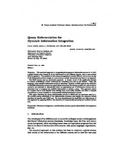
Data Integration vs. Warehousing The primary philosophical difference between a data warehouse and a virtual data integration system is essentially one of “eager” versus “lazy” evaluation (see Figure 1.1). In data warehousing, the expectation is that the data changes infrequently or that the integrated view does not need to be current — and that large numbers of expensive queries will be posed over the integrated view of the data. Hence, the full contents of the global schema are precomputed (by evaluating all source mappings), they are
4
On demand: Query executes over warehouse
Offline: ETL tool archives data periodically
Results
XML Source
Warehouse DBMS Application or Interactive User Interface
Data
ETL Tools Query over Warehouse Schema
Data
Data in Common Format and Schema
(offline) Data
Warehoused tables
Legacy Source
Relational Source
(a) Data Warehouse On demand: Query executes directly over wrapped sources Results
XML Source
Data Integration System Application or Interactive User Interface
Data
Wrappers Query over Mediated Schema
Virtual mediated schema
Data in Common Format
Data (demand-driven) Data
Legacy Source
Relational Source
(b) Virtual Data Integration System
Figure 1.1: Data warehousing (a) replicates data from sources offline and executes its queries over the warehoused data. Virtual data integration (b) presents a virtual, mediated schema but fetches the actual data on-demand from the underlying data sources.
stored in a separate “warehouse” database that will be used for querying, and significant attention is given to physical warehouse design and indexing, in order to get the best possible query performance. Refreshing the warehouse is typically relatively expensive and done offline, using ETL (extract, transform, and load) tools. Data integration addresses the case where warehousing is impractical, overly expensive, or impossible: for instance, when queries only access small portions of the data, the data changes frequently, “live” data is required, data-providing partners are
5
only willing to grant limited access to their data, or the global schema itself may be changed frequently. In fully virtual data integration, the global schema is strictly a logical or virtual entity — queries posed over it are dynamically rewritten at runtime to refer to actual data sources (based on the source mappings), and data is fetched from the sources (via wrappers) and combined. Data integration has become of increasing interest in recent years as it has matured, because it has several benefits to the implementer versus warehousing: it supports data sources that may only allow limited access to data; it supports a “live” view of the data environment; and it can present multiple versions of a mediated schema at the same time (for instance, to maintain compatibility with “legacy” queries). One potential drawback of the virtual data integration approach is that certain data cleaning and semantic matching operations between sources are too expensive to perform “on the fly,” and must be computed offline; another is that virtual data integration may heavily load the data sources. To handle these issues, an implementation whose characteristics fall between the fully precomputed model of the data warehouse and the fully virtual model of data integration may be desirable: certain data items or matching information may be cached, prefetched, or precomputed. In this thesis, I will consider all of these points (including full warehousing) to fall within the general category of data integration, but my interests lie in handling those sources that are not cached.
1.2 Query Processing for Data Integration Until very recently, the emphasis of research in data integration was on developing models [BRZZ99, ZRZB01, ROH99], mappings [DDH01, MBR01, HMH01], and translators or “wrappers” [KDW97, BFG01] for data sources; with additional work on the problem of translating or “reformulating” [LRO96, Qia96, DG97, FLM99, PL00, HIST02] queries over the mediated schema into queries over the real sources. These problems have been addressed well enough to provide a level of functionality that is sufficient for solving many real-world problems. Now that there are established algorithms and methodologies for data integration, there are two important challenges remaining to be addressed to make data integration a widespread technology: one is the problem of defining correspondences between entities at different data sources (i.e., mappings between different concepts or schema items, but also mappings be-
6
tween entities that appear in different sources with different representations); the other is the problem of developing system-building techniques that allow a data integration system to perform well enough that it can be useful in practice. Other researchers [MBR01, BHP00, DDH01, PR01] have started to address aspects of the first problem; my focus is on the second problem, developing techniques for efficiently answering data integration queries. As discussed earlier, traditional query processing deals with an environment in which statistics are computed offline and used to statically optimize a query, which can then be executed. This generally is effective in a standard database environment because the data and computing environment are under the strict control of the database, and they are thus fairly predictable and consistent. Yet even in this context, many simplifying assumptions must be made during optimization, and there are many situations in which the traditional model does poorly (e.g., in many circumstances, the optimizer accumulates substantial error in modeling complex queries). Even worse, the data integration domain has a number of features that make it substantially harder than the conventional database management system context. Data integration typically interacts with autonomous sources and externally controlled networks: it becomes difficult to model the expected performance of such data sources (sometimes even the amount of data it will return is unknown), and the performance of the network may be unexpectedly bursty. Unpredictability and inconsistency are the norm in querying remote, autonomous data sources. Furthermore, traditional query processing tends to optimize for complete results (i.e., batch-oriented queries). Many data integration applications are interactive, suggesting that early incremental results are particularly important in this context — suggesting the need for a different metric in query optimization, or at least a different set of heuristics.
1.2.1 Thesis Statement and Overview My thesis is that since the data integration domain is inherently filled with uncertainty, static optimization and deterministic execution based on existing knowledge are ill-suited for this domain — adaptive techniques can provide greatly improved performance. The central question I sought to answer is whether it is possible to develop adaptive query processing techniques that yield better performance in our domain:
7
they must be sufficiently low-overhead that they will compensate for the fact that adaptivity is inherently more expensive. I have answered this question by proposing and experimentally validating novel techniques for utilizing pipelining (defined in the next section) and adaptivity, which do indeed provide faster and more efficient query processing for data integration. In particular, I have found that three techniques are highly beneficial for integration of XML data, and in fact a necessity for good performance: (1) providing pipelined execution for streaming XML data as well as relational data; (2) using adaptive operators, such as the pipelined hash join, to accommodate variations in source data transfer rates; and (3) re-optimizing queries and dynamically splitting execution pipelines in mid-stream. I motivate, define, and briefly describe each technique below.
1.2.2 The Need for Pipelining Query execution occurs over a query plan, which describes a sequence or expression evaluation tree of query operators (as well as the algorithms to use in executing each operator). In general, any fragment of a query plan can be executed in one of two ways: as a pipeline, where control flow propagates up the operator evaluation tree one tuple at a time; or as a series of batch-oriented or blocking operators, where each operator consumes a table and outputs a table that gets materialized to disk and then fed into the next operator. Blocking has one substantial benefit: it executes a plan fragment as a sequence of separate stages, so not all of the operators’ state information must be in memory simultaneously. Furthermore, certain query operations (for instance, coalescing groups of tuples into sets with the same attribute values) must inherently be blocking, because they typically must “see” the entire table before they can compute output tuples. However, when it is feasible, pipelining has a very desirable characteristic for interactive applications like data integration: it returns initial answers much more quickly. In a traditional database, query plans are typically divided into a series of pipelines, where each pipeline is divided from the next by a blocking operation that materializes its results to disk. This allows the query processor to best use its resources to compute an answer. For an interactive application, overall speed is typically less a concern than speed in returning initial answers — so in this context, a good heuristic is to begin execution with a single pipeline, and develop a strategy for handling memory
8
overflow after some initial answers have been returned. Extending this concept slightly beyond the flow of tuples between operators, data should be incrementally processed as source data is streaming into the query processor’s operators — it should not be a requirement that the data be prefetched from all sources before query execution can begin. Data transfer time is often a significant factor in processing network-based queries. Finally, pipelining provides another benefit beyond returning fast initial answers: it enables more query operators to be running concurrently, and as a result, a query execution system has more flexibility in determining which operations should get resources at a particular time. I discuss techniques for adaptive scheduling in the next section. Pipelining has been a standard technique employed for standard relational databases, but the methodology had not been fully translated to the XML realm: in particular, an XML document sent across the network would need to be read and parsed in its entirety before any query processing could begin. One of my research contributions is a model for pipelining XML data as it is being streamed across the network — resulting in significantly improved performance, as well as more possibilities for adaptive scheduling and optimization. 1.2.3 The Need for Adaptive Scheduling An important characteristic of the physical query plans used by query execution engines is that, because they express both an order of algebraic evaluation and specify a set of deterministic algorithms to be used, they encode a physical scheduling. Generally, the scheduling of compute cycles to each query operator is done via an iterator execution model: an operator calls its child’s getNext() method when it needs a new tuple from the child, and the child in turn calls its child, etc. A given query operator algorithm consumes and returns tuples according to a predefined order that is hardcoded into the algorithm. The iterator model works very well for situations where I/O is relatively inexpensive and inherently sequential, and where free compute cycles are rare. In a standard database, most I/O operations come from the buffer manager (which often prefetches data) rather than directly from disk, and typically disk I/Os are not fully parallelizable (at least if they come from the same disk). Furthermore, if an operation is primar-
9
ily compute-bound, then context-switching from one operation to the next should only be done in an operation-aware fashion. Thus, in a standard database, execution of operations according to their own deterministic, embedded logic makes sense. The network-based query processing domain is considerably different. First, the I/O bottleneck typically resides at the data source or at some point within the middle of the network, rather than at the query engine itself — hence, overlapping of I/O operations from different sources can be done with significant benefit. Second, network I/O delays are often relatively long, which tends to increase the number of idle cycles within a particular query. Here, it makes sense not only to overlap multiple I/O operations with one another, but also to provide flexible or adaptive scheduling: the query processor should schedule any available work when a particular part of a query plan is I/O-bound and free cycles are available. I have proposed two enhanced algorithms for the standard query operations of join and union, both more appropriate for data integration because they support adaptive scheduling of work. Combined with a query optimization step that emphasizes pipelined execution, my techniques allow the query processor to significantly overlap I/O and computation for good performance. 1.2.4 The Need for Adaptive Re-optimization Conventional database query processors must make static decisions at optimizationtime about which query plan will be most efficient. A database query optimizer relies on a set of parameters defining CPU and I/O costs, as well as statistics describing general data characteristics, to calibrate its cost model so it can choose an inexpensive query plan. These cost values and statistics are typically recorded and periodically updated offline, and assumed to be stay relatively consistent between the update intervals. However, cost values and statistics may not stay consistent — CPU and I/O costs vary as DBMS server load changes, and statistics are often updated rather infrequently. As a result, the optimizer may actually choose poor plans. However, most database implementers have felt that these potential pitfalls were acceptable, especially since alternative techniques would be too difficult to design and implement. In the data integration context, the weaknesses of the standard query processing approach are exacerbated. First, data transfer speeds are unpredictable: network
10
congestion may delay data as it is sent from autonomous sources, and additionally the sources themselves may be overloaded at unexpected moments. Second, it is typically difficult to maintain statistics about the data within the sources: the sources were typically not designed to cooperate with a data integration system, and thus they do not export any sort of statistics-sharing interfaces. Ideally, the data integration system can gather statistics on its own, but this is not always possible: some sources do not hold relational data, and the amount and type of data they return will vary depending on how they are queried; some sources only expose small portions of their data on demand, in response to a specific query, making it difficult to estimate the overall amount of data at the source; some sources are updated frequently, rendering past statistics irrelevant very quickly. The problems caused by the data integration environment clearly suggest that static optimization decisions, based on pre-existing knowledge, are inadequate. Instead, I believe that a query plan must be chosen adaptively. In particular, the query processor can choose an initial query plan, which it will continue to refine as it monitors actual query execution costs and statistics. This allows the system to deal with factors that vary over the course of execution, as well as factors that stay consistent but are unknown prior to execution. My major contribution in this area is a novel set of techniques called convergent query processing, which allows an existing query plan to be changed in mid-stream, or even split into multiple stages, at virtually any point during execution. This flexibility is attained without imposing significant overhead, and I demonstrate how standard database query processing techniques can be leveraged in this context. Together, the techniques I propose in this dissertation provide great flexibility in the scheduling of query processing work, and do so with minimal overhead and early initial answers. They are especially well-suited to our target domain of data integration, and certain techniques such as convergent query processing may also be useful in more traditional database contexts.
1.3 Outline of Dissertation The remainder of this dissertation is structured as follows. Chapter 2 provides background about data integration and XML. It introduces the basic components of a data integration system and cites relevant work in these areas.
11
It also describes the basics of the most popular XML data models and query languages. Chapter 3 provides an overview of the considerations for adaptive query processing and the specific contributions of my thesis. It also presents an overview of the Tukwila data integration system, which utilizes the proposed techniques and has formed an evaluation platform for my work. In Chapter 4, I describe an XML query processing architecture for pipelined query execution, including query operators that incrementally consume data from an XML stream and produce tuples that are fed into pipelined query plan. I also present the complementary operators that convert from tuples back into XML. Chapter 5 describes the components of a query execution engine that are required for an adaptive query processing architecture. I describe the infrastructure that supports my adaptive query optimization techniques, and I present a basic set of query operators for performing joins and unions in a wide area context, with emphasis on adaptive scheduling. I present an extension to the pipelined hash join that supports overflow resolution, as well as a variant of the union for handling mirrored data sources. Chapter 6 then describes and evaluates techniques for performing adaptive reoptimization to improve a query plan at runtime. I detail an approach to re-optimizing at pipeline boundaries, and I present convergent query processing, a novel means of re-optimizing an executing pipeline. Chapter 7 describes the impact of the Tukwila system: I provide an overview of how my query processor has been used in a number of research projects and real applications at the University of Washington and in the Seattle area. I discuss related work in Chapter 8 and conclude with some ideas for future exploration in Chapter 9.
12
Chapter 2 BACKGROUND: DATA INTEGRATION AND XML The remainder of my thesis assumes a working knowledge of the basic concepts of data integration and XML. This chapter sets the context by providing the necessary background information. I begin with a discussion of the components of a data integration system and follow with a discussion of querying XML.
2.1 Data Integration System Architecture As discussed in the introduction, the key attributes of a data integration system are its ability to present an integrated, mediated schema for the user to query, the ability to translate or reformulate this query to combine information from the various data sources according to their relationships with the mediated schema, and the ability to execute this query over the various local and remote data sources. A data integration system varies somewhat from a standard database system: it has little or no physical storage subsystem and usually no capability for expressing updates, but it needs query translation capabilities and the ability to fetch data from remote sources. The typical components of a data integration system are illustrated in Figure 2.1, and they consist of the following: Application or Interactive User Interface Typically, the initiator of queries and consumer of answers will be an interactive, GUIbased user interface, custom application logic, or a web-based application. In general, this data consumer requires early initial answers so it can provide early feedback to the user. Furthermore, many applications will be posing ad-hoc, exploratory queries that may be terminated before they complete. Query Reformulator The initial query will typically be posed in terms of a mediated schema, a single unified schema. Schema mediation relies on expressing the relationships between the
13
XML Results
Cache Application or Interactive Interface
Query Reformulation Query over Mediated Schema
(Rewriting & Source Selection)
Query Processing Reformulated Query
(Optimization & Execution)
Cacheable XML Source
XML
XML
Wrapper XML
Source Descriptions
Data Source Catalog
Legacy Source Source Statistics
Dynamic XML Source
Figure 2.1: Data integration architecture diagram. The application or user interface poses a query over the mediated schema. The reformulator uses data from the data source catalog to rewrite this query to reference real data sources. The query processor finds an optimal plan for executing this query, then fetches data from the sources (in some cases through a wrapper or cache) and combines it to return the maximal set of answers.
global schema and the data sources through view definitions. Two classes of techniques have been proposed: local-as-view, which defines sources as views over the mediated schema, and global-as-view, which defines the mediated schema as a view over the sources (see [Hal01] for more details). Global-as-view mediation has the advantage that mediated-schema queries can be simply merged with the view definitions (“unfolded”) to get the full query. Local-as-view requires more complex query reformulation [LRO96, Qia96, DG97, FLM99, PL00, HIST02], but has been shown to be more expressive — thus most modern data integration systems use it (or a hybrid of the two techniques, as in [FLM99, HIST02]). Work in query reformulation algorithms has been a major focus of database researchers at the University of Washington: UW authors have contributed the bucket [LRO96] and MiniCon [PL00] algorithms. The existing work in query reformulation has been on conjunctive queries over purely relational data. However, the most natural data model for integrating multiple schemas is that of XML (see [FMN02a]), since this data model is general enough to accommodate hierarchical, object-oriented, document, and relational data sources. We expect, therefore, that a data integration query will typically be posed in XQuery [BCF+ 02], the standard query language being developed for XML. Based on recent trends in the database theory community, I expect that query reformulation will soon be extended
14
to handle more general XML data. Thus, for the purposes of my work, I have assumed the eventual creation of a query reformulator for XQuery (or a subset thereof). In fact, recent research on the Piazza project has begun to adapt the MiniCon algorithm to work with a conjunctive subset of XQuery [HIST02]. Data source catalog The catalog contains several types of metadata about each data source. The first of these is a semantic description of the contents of the data sources. A number of projects, including [DDH01, MBR01, HMH01], have focused on developing techniques for automatic or semi-automatic creation of mappings between data sources and the mediated schema of the data integration system. Data source sizes and other data distribution could also be recorded alongside the information about the mappings, but this will only feasible if the data source changes infrequently and can be “probed” in a comprehensive way; I do not expect this to be the common case. In a few cases, a system may have even further information describing the overlap between data values at different sources. A model for reasoning about overlap is described in [FKL97], and describes the probability that a data value d appears in source S1 if d is known to appear in source S2 . This can be used alongside cost information to prioritize data from certain data sources. Attempts have also been made to profile data sources and develop cost estimates for their performance over time [BRZZ99, ZRZB01], and to provide extensive models of data source costs and capabilities [LRO96, CGM99, LYV+ 98, ROH99]. Query processor The query processor takes the output of the query reformulator — a query over the actual data sources (perhaps including the specification of certain alternate sources) — and attempts to optimize and execute it. Query optimization attempts to find the most desirable operator evaluation tree for executing the query (according to a particular objective, e.g., amount of work, time to completion), and the query execution engine executes the particular query plan output by the optimizer. The query processor may optionally record statistical profiling information in the data source catalog. In this dissertation, I describe how adaptive techniques and pipelining can be used to produce an efficient query processor for network-bound XML data.
15
Wrappers Initial work on data integration predates the recent efforts to standardize data exchange. Thus, every data source might have its own format for presenting data (e.g., ODBC from relational databases, HTML from web servers, binary data from an objectoriented database). As a result, one of the major issues was the “wrapper creation problem.” A wrapper is a small software module that accepts data requests from the data integration (or mediator) system and fetches the requested data from the data source; then converts from a data source’s underlying representation to a data format usable by the mediator. Significant research was done on rapid wrapper creation, including tools for automatically inducing wrappers for web-based sources based on a few training examples [KDW97, BFG01], as well as toolkits for easily programming web-based wrappers [SA99, LPH00]. Today, the need for wrappers has diminished somewhat, as XML has been rapidly adopted as a data exchange format for virtually any data source. (However, the problem has not completely disappeared, as legacy sources will still require wrappers to convert their data into XML.) Data Sources The data sources in an integration environment are likely to be a conglomeration of pre-existing, heterogeneous, autonomous sources. Odds are high that none of these systems was designed to support integration, so facilities for exchanging metadata and statistics, estimating costs, and offloading work are unlikely to be present. Sometimes the sources will not even be truly queryable, as with XML documents or spreadsheets. Additionally, in many cases the sources are controlled by external entities who only want to allow limited access to their data and computational resources. At times, these access restrictions may include binding patterns, where the source must be queried for a particular attribute value before it returns the corresponding tuples 1 . The data sources may be operational systems located remotely and running with variable load — hence, the data integration system will often receive data from a given source at an indeterminate and varying rate. The data integration system must be able to accommodate these variations, and should be able to “fall back” to mirrored sources or caches where appropriate. 1
An instance of this is a web form from Amazon.com, where the user must input an author or title before the system will return any books
16
Another important issue related to external data sources is that of semantic matching of entities. Multiple data sources may reference the same entity (for instance, a user may be a member of multiple web services). Frequently, these different data sources will have a different representation of identity, and an important challenge lies in determining whether two entities are the same or different. This problem is far from being solved, but some initial work has been done on using information retrieval techniques for finding similarity [Coh98] and on probabilistic metrics [PR01]. In many cases, however, semantic matching is straightforward enough to be done in exact-match fashion, or users may supply matching information. For these situations, we merely need a common data format. XML has emerged as the de facto standard for exchanging information, and virtually any demand-driven data integration scenario is likely to be based on XML data requested via HTTP. Most applications already support some form of XML export capabilities, but legacy applications may require wrappers to export their data in XML form. A key characteristic of XML is its ability to encode structured or semi-structured information of virtually any form: relational and object-oriented data, text documents, even spreadsheets and graphics images can be encoded in XML.
2.2 The XML Format and Data Model XML originates in the document community, and in fact it is a simplified subset of the SGML language used for marking up documents. At a high level, XML is a very simple hierarchical data format, in which pairs of open- and close-tags and their content form elements. Within an element, there may be nested elements; furthermore, each element may have zero or more attributes. From a database perspective, the difference between an attribute and an element is very minor — attributes may only contain scalar values, an attribute may occur only once per element, and attributes are unordered with respect to one another. Elements, on the other hand, may be repeated multiple times, may include element or scalar data, and are ordered with respect to one another. An example XML document representing book data is shown in Figure 2.2. An XML document is fully parsable and “well-formed” if every open-tag has a matching close-tag and the details of the XML syntax are followed. However, typically the XML document structure is constrained by a schema. There are two standards for specifying schemas in XML: DTDs and XML Schemas.
17
Readings in Database Systems Stonebraker Hellerstein 123-456-X Transaction Processing Bernstein Newcomer 235-711-Y Morgan Kaufmann San Mateo CA Figure 2.2: Sample XML document representing book and publisher data.
The DTD, or Document Type Definition, establishes constraints on XML tags, but does so in a very loose way. A DTD is essentially an EBNF grammar that restricts the set of legal XML element and attribute hierarchies. The DTD also explicitly identifies two special types of attributes: IDs and IDREFs. An ID-typed attribute has a unique value for each document element in which it is contained — this forms, in essence, a key within the scope of a document. IDREF and IDREFS-typed attributes, correspondingly, form references to particular IDs within a document. An IDREF contains a single reference to an ID; an IDREFS attribute contains a list of space-delimited IDs. The XML specification mandates that no IDREFs within a document may form dangling references. XML Schema is a more recent standard intended to supplant the DTD. The primary benefits of Schema are support for element types and subclassing, support for richer type information about values (e.g., integers, dates, etc.), and support for keys and foreign keys. Unfortunately, Schema is a very complex standard with many related
18
db
book ISB
any
publisher #8 autho e l rs tit
123-456-X
#5 Readings Hellerstein In Database Stonebraker Systems
#9
#10
#11 n ame #13
e
#4 na me
mkp
na m
#7
nam e
N
#6
comp
bo
city
nam
ok
publisher
N ISB
#3
e
e
titl
editors
#2
#1
#14
#15
sta
te #16
#12 Principles 235-711-Y San Mateo Newcomer of Transaction Morgan Kaufmann CA Bernstein Processing
Figure 2.3: XML-QL graph representation for Figure 2.2. Dashed edges represent IDREFs; dotted edges represent PCDATA.
but slightly different idioms (e.g., different types of inheritance, support for structural subtyping and name subtyping), and there is no clean underlying data model that comes with the standard. There have been numerous proposals for an XML data model, but two are of particular interest to us. The first proposal, a mapping from XML into the traditional semistructured data model, is interesting because it provides graph structure to an XML document; however, it does not capture all elements of the XML specification. The second proposal, the W3C XML Query data model, is tree-based but incorporates all of the different details and idiosyncrasies of the XML specification, including processing instructions, comments, and so forth. The XML Query data model is an attempt to define a clean formalism that incorporates many of the core features of XML Schema. 2.2.1 The XML-QL Data Model Today, with the advent of proposed standards, the XML-QL query language [DFF+ 99] has lost favor, so one could argue that its data model is irrelevant. However, the data model is a mapping from XML to a true semi-structured data model, and thus it has some interesting features that are missing from recent standards — features that may be important for certain applications. In the XML-QL data model, each node receives a unique label (either the node’s
19
db book
publisher="m
kp"
book
isbn
publisher="mkp"
ID="mkp"
company
editor
title
editor Stonebraker
Readings In Database Systems
author
title 123-456-X
Hellerstein
author
isbn Bernstein Newcomer
Principles of Transaction 235-711-Y Processing
name
city
state
San Mateo CA Morgan Kaufmann
Figure 2.4: Simplified XQuery data model-based representation for Figure 2.2. Dashed edges illustrate relationships defined by IDREFs; dotted edges point to text nodes.
ID attribute or a system-generated ID). A given element node may be annotated with attribute-value pairs; it has labeled edges directed to its sub-elements and any other elements that it references via IDREF attributes. Figure 2.3 shows the graph representation for the sample XML data of Figure 2.2. Note that IDREFs are shown in the graph as dashed lines and are represented as edges labeled with the IDREF attribute name; these edges are directed to the referenced element’s node. In order to allow for intermixing of “parsed character” (string) data and nested elements within each element, we create a PCDATA edge to each string embedded in the XML document. These edges are represented in Figure 2.3 as dotted arrows pointing to leaf nodes. XML-QL’s data model only has limited support for order: siblings have indices that record their relative order, but not absolute position, so comparing the order of arbitrary nodes is difficult and requires recursive comparison of the ancestor nodes’ relative node orderings (starting from the root). Furthermore, XML-QL’s data model does not distinguish between subelement edges and IDREF edges — therefore, a given graph could have more than one correct XML representation. 2.2.2 The XML Query Data Model The World Wide Web Consortium’s XML Query (XQuery) data model [FMN02b] is based on node-labeled trees, where IDREFs exist but must be dereferenced explicitly. The full XQuery model derives from XML Schema [XSc99], or at least a cleaner ab-
20
straction of it called MSL [BFRW01]. This data model has many complexities: elements have types that may be part of a type hierarchy; types may share portions of their substructure (“element groups”); elements may be keys or foreign keys; scalar values may have restricted domains according to specific data types; and the model also supports XML concepts such as entities, processing instructions, and even comments. Furthermore, any node in the XQuery data model has implicit links to its children, its siblings, and its parent, so traversals can be made up, down, or sideways in the tree. For the purposes of this thesis, most of XQuery’s type-related features are irrelevant to processing standard, database-style queries, so I will discuss only a limited subset of the XQuery data model, which focuses on elements, attributes, and character data and which includes order information. Figure 2.4 shows a simplified representation of our example XML document using this data model, where a left-to-right preorder traversal of the tree describes the order of the elements.
2.3 Querying XML Data
During the past few years, numerous query languages for XML have been proposed, but recently the World Wide Web Consortium has attempted to standardize these with its XQuery language specification [BCF+ 02]. The XQuery language is designed to extract and combine subtrees from one or more XML documents. The basic XQuery expression consists of a For-Let-Where-Return clause structure (commonly known as a “flower” expression): the For clause provides a series of XPath expressions for selecting input nodes, the Let clause similarly defines collection-valued expressions, the Where clause defines selection and join predicates, and the Return clause creates the output XML structure. XQuery expressions can be nested within a Return clause to create hierarchical output, and, like OQL, the language is designed to have modular and composable expressions. Furthermore, XQuery supports several features beyond SQL and OQL, such as arbitrary recursive functions. XQuery subsumes most of the operations of SQL, and general processing of XQuery queries is extremely similar, with the following key differences.
21
FOR $b $t $n RETURN
{ IN document("books.xml")/db/book, IN $b/title/data(), IN $b/(editor|author)/data() { $n } { $t } } Figure 2.5: XQuery query that finds the names of people who have published and their publications. The For clause specifies XPath expressions describing traversals over the XML tree, and binds the subtrees to variables (prefixed with dollar signs).
Input Pattern-Matching (Iteration) XQuery execution can be considered to begin with a variable binding stage: the For and Let XPath expressions are evaluated as traversals through the data model tree, beginning at the root. The tree matching the end of an XPath is bound to the For or Let clause’s variable. If an XPath has multiple matches, a For clause will iterate and bind its variable to each, executing the query’s Where and Return clause for each assignment. The Let clause will return the collection of all matches as its variable binding. A query typically has numerous For and Let assignments, and each legal combination of these assignments is considered an iteration over which the query expression should be evaluated. An example XQuery appears in Figure 2.5. We can see that the variable $b is assigned to each book subelement under the db element in document books.xml; $t is assigned the title within a given $b book, and so forth. In my thesis work, I assume an extended version of XPath that allows for disjunction along any edge (e.g., $n can be either an editor or author), as well as a regular-expression-like Kleene star operator (not shown). In the example, multiple match combinations are possible, so the variable binding process is performed in the following way. First, the $b variable is bound to the first occurring book. Then the $t and $n variables are bound in order to all matching title and editor or author subelements, respectively. Every possible pairing of $t and $n values for a given $b binding is evaluated in a separate iteration; then the
22
Stonebraker Readings in Database Systems Hellerstein Readings in Database Systems Bernstein Transaction Processing Newcomer Transaction Processing Figure 2.6: The result of applying the query from Figure 2.5 to the XML data in Figure 2.2. The output is a series of person-publisher combinations, nested within a single result root element.
process is repeated for the next value of $b. We observe that this process is virtually identical to a relational query in which we join books with their titles and authors — we will have a tuple for each possible htitle, editor|authori combination per book. The most significant difference is in the terminology; for XQuery, we have an “iteration” with a binding for each variable, and in a relational system we have a “tuple” with a value in each attribute. XML Result Construction The Return clause specifies a tree-structured XML constructor that is output on each iteration, with the variables replaced by their bound values. Note that variables in XQuery are often bound to XML subtrees (identified by their root nodes) rather than to scalar values. The result of the example query appears in Figure 2.6. One of the primary idioms used in XQuery is a correlated flower expression nested within the Return clause. The nested subexpression returns a series of XML elements
23
that satisfy the correlation for each iteration of the outer query — thus, a collection of elements gets nested within each outer element. This produces a “one-to-many” relationship between parent and child elements in the XML output. Note that this particular type of query has no precise equivalent in relational databases, but it has many similarities to a correlated subquery in SQL. Traversing Graph Structure Finally, as we pointed out earlier in our discussion of the XML data model, some XML data makes use of IDREF attributes to represent links between elements (the dashed lines in Figure 2.3). IDREFs allow XML to encode graph-structured as well as treestructured data. However, support for such capabilities in XQuery is limited: while XQuery has “descendant” and “wildcard” specifiers for selecting subelements, its -> dereference operator only supports following of single, specified edges. These restrictions were presumably designed to facilitate simpler query processing at the expense of query expressiveness. For applications that require true graph-based querying, extensions to XQuery may be required, and these extensions will give us a data model that looks more like that for XML-QL. We discuss these features in more detail in Chapter 4. 2.3.1 Querying XML for Data Integration To this point, we have discussed the general principles of querying an XML document or database, including data models, query languages, and unique aspects. Our discussion has assumed that the XML data is available through a local database or a materialized data source, e.g., an XML document on a local web server. However, the data integration context provides an interesting variation on this pattern: sometimes XML data may be accessible only via a specific dynamic query, as the result of a “virtual XML view” over an underlying data source (e.g., an XML publishing system for a relational database, such as [FTS99, CFI+ 00], or a web forms interface, such as those at Amazon.com). This query may need to request content from the data source according to a specific value (e.g., books from Amazon with a particular author). In other words, a data integration system may need to read a set of values from one or more data sources, then use these to generate a dynamic query to a “dependent” data source, and then combine the results to create a query answer. XQuery currently
24
supports a limited form of dynamic queries, based on CGI requests over HTTP, and the Working Group is considering the addition of special functions for fully supporting these features under other protocols such as SOAP. Now that the reader is familiar with the basic aspects of data integration and XML query processing, we focus on the problem of XML query processing for data integration.
25
Chapter 3 QUERY PROCESSING FOR DATA INTEGRATION The last chapter presented the basic architecture of a data integration system and discussed several motivations for adopting the XML data format and data model standards. The construction of data integration systems has been a topic of interest to both of my advisors, who developed the Information Manifold [LRO96] and Razor [FW97]. These systems focused on the problems of mapping, reformulation, and query planning for relational data. My thesis project, Tukwila, builds upon the techniques developed for these systems and the rest of the data integration community, with a new emphasis: previous work established the set of capabilities that a basic data integration system should provide and developed techniques for effective semantic medation. However, they typically focused on issues other than providing the level of scalability and performance necessary to be used in real applications. In the data integration domain, queries are posed over multiple autonomous information sources distributed across a wide-area network. In many cases, the system interacts directly with the user in an ad-hoc query environment, or it supplies content for interactive applications such as web pages. The focus of my thesis has been on addressing the needs of this type of domain: building a data integration query processing component that provides good performance for interactive applications, processes XML as well as relational data, and handles the unique requirements of autonomous, Internet-based data sources. As I discuss in previous chapters, modern query processors are very effective at producing well-optimized query plans for conventional databases, and they do this by leveraging I/O cost information as well as histograms and other statistics to compare alternative query plans. However, data management systems for the Internet have demonstrated a pressing need for new techniques. Since data sources in this domain may be distributed, autonomous, and heterogeneous, the query optimizer will often not have histograms or any other quality statistics. Moreover, since the data is only accessible via a wide area network, the cost of I/O operations is high, unpredictable, and variable. I propose a combination of three techniques, which can be broadly classified as
26
adaptive query processing, to mitigate these factors: 1. Data should be processed as it is streaming across the network (as is done in relational databases via pipelining) 1 . 2. The system should employ adaptive scheduling of work, rather than using a deterministic and fixed strategy, to accommodate unpredictable I/O latencies and variable data flow rates. 3. The system should employ adaptive plan re-optimization, where the query processor adapts its execution strategy in response to new knowledge about data sizes and transfer rates as the query is being executed. In the remainder of this chapter, I provide a more detailed discussion of how these three aspects interrelate. I begin with a discussion of the adaptive query processing space and where my work falls within this space, then in Section 3.2 I provide a sketch of how my thesis contributions in adaptive query processing solve problems for data integration, and I conclude the chapter with an overview of my contributions in the Tukwila system, which implements the adaptive techniques of my thesis.
3.1 Position in the Space of Adaptive Query Processing Adaptive query processing encompasses a variety of techniques, often with different domains in mind. While I defer a full discussion of related work to Chapter 8, it is important to understand the goals of my thesis work along several important dimensions: Data model To this point, most adaptive query processing techniques have focused on a relational (or object-relational) data model. While there are clearly important research areas within this domain, other data models may require extensions to these techniques. In particular, XML, as a universal format for describing data, allows for hierarchical and graph-structured data. I believe that XML is of particular interest 1
Note that our definition of “streaming” does not necessarily mean “infinite streams,” as with some other recent works, e.g. [DGGR02a].
27
within a data integration domain, for two reasons. First, XML is likely to be the predominant data format for integration, and it poses unique challenges that must be addressed. Second, the basic concepts from relational databases often are insufficient for XML processing. For instance, there has been no means of “pipelining” XML query processing as the data streams across the network 2 . As a second example, the notions of selectivity and cardinality have a slightly different meaning in the XML realm, since the number of “tuples” to process depends on the XPath expressions in the query.
Remote vs. local data Traditional database systems have focused on local data. Recent work in distributed query processing has focused on techniques for increasing the performance of network-bound query applications, including [UFA98, UF99, IFF+ 99, AH00, HH99]. The focus of my thesis has been on remote data, although many of the techniques can be extended to handle local data as well.
Large vs. small data volumes Data warehouses and many traditional databases concentrate on handling large amounts of data (often in the tens or hundreds of GB). In contrast, most previous work on data integration systems and distributed databases has concentrated on small data sources that can easily fit in main memory. My focus is on “mid-sized” data sources: sources that provide tens or hundreds of MB of data, which is enough to require moderate amounts of computation but which is still small enough to be sent across typical local-area and wide-area networks. I believe that typically, most data sources will be able to filter out portions of their data according to selection predicates, but that they will be unlikely to perform joins between their data and that of other sources — hence, the amount of data sent is likely to be nontrivial.
First vs. last tuple For domains in which the data is used by an application, the query processor should optimize for overall query running time — the traditional focus of database query optimizers. Most of today’s database systems do all of their optimization in a single step; the expectation (which does not generally hold for large query plans [AZ96] or for queries over data where few statistics are available) is that the optimizer has sufficient knowledge to build an efficient query plan. The INGRES optimizer [SWKH76] and techniques for mid-query re-optimization [KD98] often yield 2
SAX parser events can be viewed as a form of pipelining, but they do not do query processing.
28
better running times, because they re-optimize later portions of the query plan as more knowledge is gained from executing the earlier stages. I have studied re-optimization both as a way to speed up total running time (last tuple) and as a way of improving time to first tuple. My work has also emphasized pipelined execution as a heuristic that typically speeds time to first tuple. Re-use of results and statistics Data may often be prefetched and cached by the query processor, but the system may also have to provide data freshness guarantees. Caching and prefetching are well-studied areas in the database community, and the work on rewriting queries over views [Hal01] can be used to express new queries over cached data, rather than going to the original data sources. My thesis work does not directly investigate caching, but our work on Piazza (see Chapter 7) investigates the use of caching mechanisms in network-based query processing. Related to caching of data, it is also possible to “learn” statistical models of the content at data sources, as in [CR94], or patterns of web-source access costs, as in [BRZZ99, ZRZB01]. My thesis work can take advantage of cached results or statistics when they are available, but the emphasis is on working well even when they are not.
3.2 Adaptive Query Processing for Data Integration As mentioned above, I have proposed a three-pronged strategy to providing a comprehensive solution to network-based query processing. I describe these dimensions in the following subsections, and I describe how my contributions differ from previous techniques within each dimension. A more comprehensive section on related work appears in Chapter 8. 3.2.1 Pipelining XML Data XML databases [Aea01, XLN, Tam, GMW99, FK99b, SGT+ 99, AKJK+02, KM00, BBM+ 01] typically map XML data into an underlying local store — relational, object-oriented, or semistructured — and do their processing within this store. For a network-bound domain where data may need to be re-read frequently from autonomous sources to guarantee “freshness,” this materialization step would provide very poor performance. Furthermore, deconstructing and reconstructing XML introduces a series of complex operations that limit opportunities for adaptivity. Thus it is imperative that an XML
29
data integration system not materialize the data first, but instead support processing of the data directly. Contrasting with databases, the tools from the XML document community (in particular, XSLT processors) have been designed to work on XML data without materializing it to disk — they typically build a Document Object Model (DOM) parse tree of the single XML document to be processed, and then they match XSLT templates against this document and return a new DOM tree. Note that they are limited by main memory and they typically only work over a single document. More significantly, they do not provide incremental evaluation of queries: first the document is read and parsed, then it is walked, and finally output is produced. Since network data transfer and XML parsing are both slow, it is desirable to incrementally pipeline the data as it streams in, much as a relational engine can pipeline tuples as they stream in. This capability would improve pure performance, and it would also enhance the number of possibilities for adaptive scheduling of work and for re-optimization, since more concurrent operations would be occuring. In order to provide incremental, pipelined evaluation of XML queries, a system must be able to support efficient evaluation of regular path expressions over the incoming data, and incremental output of the values they select. Regular path expressions are a mechanism for describing traversals of the data graph using edge labels and optional regular-expression symbols such as the Kleene-star (for repetition) and the choice operator (for alternate subpaths). Regular path expressions bear many similarities to conventional object-oriented path expressions, and can be computed similarly; however, the regular expression operators may require expensive operations such as joins with transitive closure. The first contribution of my thesis is a query processing architecture that focuses on pipelining XML data in a way that is similar to relational query execution. A key contribution is the x-scan operator, which evaluates XPath expressions across incoming XML data, and which binds query variables to nodes and subgraphs within the XML document. X-scan includes support for both tree- and graph-structured documents, and it is highly efficient for typical XML queries. It combines with the other adaptive query features proposed in my thesis to rapidly feed data into an efficient query plan, and thus return initial data to the user as quickly as possible.
30
3.2.2 Adaptive Operator Scheduling A physical query plan generally contains both an algebraic order of evaluation (i.e., an evaluation tree specifying operator precedence) for the query data, as well as a set of physical algorithms that establish a physical order of evaluation (e.g., nested loops join defines that the “inner” table be iterated over before the “outer” table). Adaptive operator scheduling techniques preserve the current algebraic query plan, but modify which operators are physically scheduled first or which tuples are processed earliest. An example of an adaptive operator is the pipelined hash join, or double pipelined join [RS86, WA91], which runs the child subtrees of the join and their parent in separate concurrent threads (which are scheduled by the operating system or the database itself). Another example is one aspect of query scrambling [UFA98], which reschedules a portion of a query plan when an initial delay is encountered. Finally, dynamic pipeline scheduling [UF01] allows a query plan to prioritize the processing of certain tuples to produce early output. Adaptive scheduling produces no benefits if the query is completely I/O-bound and all data has been fully processed. On the other hand, it is extremely beneficial for queries that are what might be termed “scheduling-bound” — where the default scheduling prevents the plan from doing work it might otherwise be able to perform — and it is also helpful if the query is CPU-bound and the system wishes to prioritize certain results. A key characteristic of operator scheduling is that it affects query performance over the currently available tuples, but does not affect the overall amount of work the CPU must perform to complete the query. Hence, a scheduling change is in some sense a “low-risk” decision, as it does not incur a future penalty. In data integration, adaptive scheduling can be extremely beneficial, because a complex pipelined query plan typically encounters situations in which a particular query operator is I/O-bound, but some other operator could be doing work. Here, the query processor can block the I/O-bound operator and switch to the one that can make progress, and it can do this without needing to consider the possibility of incurring a penalty. My contributions in the area of adaptive operator scheduling are a variant of the pipelined hash join that supports dynamic destaging when it runs out of memory, as well as a query operator called the dynamic collector, which adaptively reads tuples
31
from mirrored or overlapping sources according to source priority and availability. 3.2.3 Adaptive Query Plan Re-Optimization Changing the algebraic plan order (or the physical algorithms being used within the query plan) is much more significant than changing plan scheduling, because this has a long-term effect on overall plan performance. This is because future tuples must be processed not only within the new plan, which has a set of intermediate results with which it must be combined, but they must also be combined with all data in previous plans. Depending on the sizes of the intermediate results in all of the plans, some computation may be extremely inexpensive, and other computation may be extremely costly. The decision to change a plan should generally be made when new selectivity or cardinality values are discovered and the original cost estimates for the query are known to be based on invalid assumptions and likely to lead to high cost. Instances of plan modification include the operator synthesis stage of query scrambling [UFA98], dynamic re-optimization [KD98], the eddy [AH00], and convergent query processing [IHW]. Changing a query plan can be a costly operation, and it tends to waste work, so most prior techniques enabled adaptivity between pipelines — when a fragment of a query plan completed, techniques such as choose nodes or dynamic re-optimization could change the remainder of the query plan. This prevented the possibility of redoing computation, and meant that the emphasis of these efforts was on choosing the optimal points at which to break pipelines, as well as on deciding when to re-optimize. The initial Tukwila system built similar capabilities into the query optimizer and execution engine. However, my co-authors and I found several significant problems: • Re-optimization is required because the query optimizer generally has too few statistics to select a good query plan. Unfortunately, in many cases, it also has too few statistics to select a good point at which to break a pipeline. • One of the desiderata for data integration is early initial answers. Breaking a query plan into multiple pipelines increases the amount of time before a first answer is delivered. • Even with re-optimization, query execution might take a very long time if the initial pipeline was poorly chosen.
32
Clearly, a better solution would be one that could re-optimize the current pipeline, rather than merely a future one. Not only would this eliminate the need for an a priori decision about where to break the pipeline, but it would actually allow the entire query to be executed in a single pipeline (producing faster initial answers), and it would also allow the system to switch from a bad initial plan to a better one. It is important, however, that this set of adaptive capabilities be provided in a way that does not detract from average-case performance. More specifically, we would also like the following features: • The ability to take advantage of any existing statistics or samples from tables when they are available. • Low overhead beyond that of standard query processing techniques. • Efficient re-use of available data, and minimal re-execution of work. • The ability to support not only standard select, project, and join operators, but also aggregation optimizations, and potentially to use more sophisticated query rewrite techniques (e.g., [MP94]). The eddy algorithm of [AH00] supports frequent dynamic re-optimization of a query plan, but focuses on re-optimizing as each new tuple that enters the system. As a result, it relies on a greedy heuristic that does not support aggregation or complex queries, and one which cannot take advantage of existing statistics. Furthermore, eddies, at least in their current implementation, are less efficient than traditional query processing techniques because of the inherent overhead in re-optimization and in routing tuples through operators. The third contribution of my thesis is a technique called convergent query processing, which allows for adaptive re-optimization that meets the basic desiderata listed above. It can take advantage of existing cost information and data statistics, but can also infer statistics and costs for situations where it does not have them. It provides great flexibility in the kinds of re-optimizations that are possible, but minimizes redundant work. Finally, the decision making can be done with low overhead, as the system can re-optimize in the background and at periodic intervals.
33
Optimization Costannotated Optimizer Phase Plans
Query Candidate Optimizer Plans
Execution P0 P0
P1
Physical Phase P1 Plans Results Executing Phase Plan
Global Statistics Execution Status
Cost Estimates
Status Monitor Re-optimization Trigger
Re-Opt. Trigger
Rule Trigger
Event Handler
Figure 3.1: Architecture diagram for Tukwila query processor: Tukwila contains tightly interlinked optimization and execution components. The optimizer can be re-invoked by triggering certain rules, or when a status monitor determines that a plan should be re-optimized in mid-stream.
3.3 The Tukwila Data Integration System: An Adaptive Query Processor
In order to validate the techniques proposed in my thesis, both experimentally and for real-world applications, I have built an adaptive query processor as the core of the Tukwila data integration system. The current Tukwila implementation is a complete data integration environment except that it is not typically coupled with a query reformulator module: it accepts reformulated XQueries over XML data sources, it requests data from these sources via HTTP or NFS requests, and it combines the source XML to form new results. In other work, my co-authors and I have also combined the Tukwila system with the MiniCon reformulator algorithm of [PL00] to form a complete system with a mediated schema, which works for conjunctive relational queries. (Tukwila has also been the query processor for a number of other projects at the University of Washington, as I discuss in Chapter 7.)
34
3.3.1 Novel Architectural Features The focus of my thesis work has been on the query processing component of Tukwila, illustrated in Figure 3.1. So far as I am aware, the Tukwila query processor is the first system to be engineered with the express goal of building an adaptive query processor. Key architectural aspects of Tukwila include the following: • An architecture that emphasizes pipelined query execution, in order to produce early first results. Our system typically begins with a single pipelined query plan, and it can read and process XML as it streams across the network. Since a single pipeline may run out of resources, my architecture include capabilities for handling memory overflow and for adaptively splitting a single pipeline into multiple stages once a significant portion of computation has completed. • Support for multithreaded execution of queries, in order to facilitate adaptive scheduling. Unlike most traditional, iterator-based query processors, my system is not forced to rely on deterministic scheduling, and instead it can selectively attempt to overlap I/O and computation to more effectively utilize available data and resources. • Novel algorithms for network-based and pipelined query processing, including: (1) a variant of the pipelined hash join [RS86] that supports overflow resolution and the dynamic collector, (2) a specialized version of the relational union that, upon data source failure, can switch from the original data source to its mirrors or alternates, (3) an XPath pattern-matching operator, x-scan, which produces variable bindings in pipelined fashion over streaming XML data, and (4) an operator, indirect-scan that generalizes the relational dependent join operator for a web- and XML-oriented environment. • Mechanisms for efficiently switching query plans in mid-execution of a pipeline, as well as at the interface between two separate pipelines. One of the key challenges in building the Tukwila execution engine was providing mechanisms for efficiently passing data along pipelines (using techniques such as sharing space in the buffer pool between operators), but also enabling a query plan to be modified in mid-execution.
35
• Close coupling between the query optimization and execution components. The optimizer and execution engine expose their data structures to a status monitor that periodically reads query execution cost and selectivity information and uses this to update the query optimizer’s cost model. If the actual values diverge significantly from the estimates, a query re-optimization operation may be triggered in the background. • An event handler for responding to important runtime events. The event handler provides a way of responding to data source failures, network delays, and memory overflow. The event handler is capable of initiating a complete re-optimization of the query. Note that the event handler operates at a lower granularity than a handler for traditional database triggers or active rules: it responds to events at the physical level rather than the logical level, and it can also modify the behavior of query operators or initiate a change in query plans. • An extended version of the System-R cost-based optimizer algorithm ([SAC+ 79]) that can be used not only to create initial query plans, but also to periodically reoptimize an executing query plan when better statistical information is available. • Support within both the cost-based query optimizer and the query execution system for sharing of data structures across different query plans within an execution sequence. These capabilities are used to avoid repeating computation of results in a query execution sequence that consists of multiple plans. Adaptive behavior during query execution is key in situations where I/O costs are variable and unpredictable. When data sizes are also unpredictable, it is unlikely that the query optimizer will produce a good query plan, so it is important to be able to modify the query plan being executed. As a result, Tukwila supports incremental reoptimization of queries during particular plan execution points. In the following chapters, I provide a detailed discussion of each of the novel aspects of my work, and supplement this discussion with an experimental evaluation of the techniques within the Tukwila system.
36
Chapter 4 AN ARCHITECTURE FOR PIPELINING XML STREAMS For many years, a wide variety of domains, ranging from scientific research to electronic commerce to corporate information systems, have had a great need to be able to integrate data from many disparate data sources at different locations, controlled by different groups. Until recently, one of the biggest obstacles was the heterogeneity of the sources’ data models, query capabilities, and data formats. Even for the most basic data sources, custom wrappers would need to be developed for each data source and each data integration mediator, simply to translate mediator requests into data source queries, and to translate source data into a format that the mediator can handle. The emergence of XML as a common data format, as well as the support for simple web-based query capabilities provided by related XML standards, has suddenly made data integration practical in many more cases. XML itself does not solve all of the problems of heterogeneity — for instance, sources may still use different tags or terminologies — but often, data providers come to agreement on standard schemas, and in other cases, we can use established database techniques for defining and resolving mappings between schemas. As a result, XML has become the standard format for data dissemination, exchange, and integration. Nearly every data management-related application now supports the import and export of XML, and standard XML Schemas and DTDs are being developed within and among enterprises to facilitate data sharing (instances of these are published at the BizTalk and OASIS web sites 1 ). Language- and system-independent protocols such as the various web services standards, Microsoft’s .NET [NET01] initiative, and Sun’s JXTA [JXT01] peer-to-peer protocols use XML to represent transactions and data. Processing and integrating XML data poses a number of challenges. In many data integration applications, XML is merely a “wire format,” the result of some view over a live, dynamic, non-XML source. In fact, the source may only expose subsets of its data as XML, via a query interface with access restrictions, e.g., the source may only 1
See www.biztalk.org and www.xml.org.
37
return data matching a selection value, as in a typical web form. Since the data is controlled and updated externally and only available in part, this makes it difficult or impossible to cache the data. Moreover, the data sources may be located across a wide-area network or the Internet itself, so queries must be executed in a way that is resilient to network delays. Finally, the sources may be relatively large, in the 10s to 100s of MB or more, and that may require an appreciable amount of time to transfer across the network and parse. We refer to these types of data sources as “networkbound”: they are only available across a network, and the data can only be obtained through reading and parsing a (typically finite) stream of XML data. To this point, integration of network-bound, “live” XML data has not been wellstudied. Most XML work in the database community has focused on constructing XML repositories and warehouses [Aea01, XLN, Tam, GMW99, FK99b, AKJK+02, KM00, BBM+ 01, SGT+ 99], exporting XML from relational databases [FTS99, FMS01a, CFI+ 00], adding information retrieval-style indexing techniques to databases [NDM+ 01, FMK00], and on supporting query subscriptions or continuous queries [Aea01, CDTW00, AF00] that provide new results as documents change or are added. Clearly, both warehousing and indexing are useful for storing, archiving, and retrieving file-based XML data or documents, but for many integration applications, support for queries over dynamic, external data sources is essential. This requires a query processor that can request data from each of the sources, combine this data, and perhaps make additional requests of the data sources as a result. To the best of my knowledge, no existing system provides this combination of capabilities. The Web community has developed a class of query tools that are restricted to single-documents and not scalable to large documents. The database community’s web-based XML query engines, such as Niagara and Xyleme, come closer to meeting the needs of data integration, but they are still oriented towards smaller documents (which may be indexable or warehoused), and they give little consideration to processing data from slow sources or XML that is larger than memory. As discussed in previous chapters, query processing for data integration poses a number of challenges, because the data is not tightly controlled or exclusively used by the data integration system. The query optimizer will often have little or no access to statistics about the data, and it likely has a very limited model of the data source’s performance. The lack of initial knowledge and the continued variation in conditions
38
suggest that static query optimization is inappropriate for the data integration domain. Later in this dissertation, I present techniques for improving performance by adapting the query plan in mid-execution and for exploiting parallelism and flexible scheduling of its constituent operators. However, even without a detailed discussion of these techniques, it is evident that the best execution model for network-bound data is one in which data can be read off the input stream and immediately pipelined through the query plan. This model presents a number of significant benefits for data integration and for enabling adaptivity: • A single execution pipeline does not require materialization operations, or preparsing or preprocessing of an XML document, so initial answers will be returned more quickly. This satisfies an important desideratum for interactive data integration applications. • A single pipeline provides the most opportunities for exploiting parallelism and for flexibly scheduling the processing of tuples. • A single pipeline processes all of the data sources at once, providing the most information about the data distributions and performance of the data sources, and about the selectivity of query subplans. Hence, it provides the most opportunities for learning about and adapting to query execution costs. Pipelining and adaptive query processing techniques have largely been confined to the relational data model. One of the contributions of this chapter is a new XML query processing architecture that emphasizes pipelining the XML data streaming into the system, and which facilitates a number of adaptive query processing techniques. As described in Chapter 2, XML queries operate on combinations of input bindings: patterns are matched across the input document, and each pattern-match binds an input tree to a variable. The query processor iterates through all possible combinations of assignments of bindings, and the query operators are evaluated against each successive combination. At first glance, this seems quite different from the tuple-oriented execution model of the relational world, but a closer examination reveals a useful correspondence: if we assign each attribute within a tuple to a variable, we can view each legal combination of variable assignments as forming a tuple of binding values (where the values are XML trees or content). In this chapter, I describe an XML query
39
processing architecture, implemented in the Tukwila system, which exploits the correspondence between the relational and XML processing models in order to provide adaptive XML query processing capabilities, and thus to support efficient networkbound querying, even in the presence of delays, dynamic data, and source failures. This architecture includes the following novel features: • Support for efficient processing of scalar and structured XML content. Our architecture maps scalar (e.g., text node) values into a tuple-oriented execution model that retains the efficiencies of a standard relational query engine. Structured XML content is mapped into a Tree Manager that supports complex traversals, paging to disk, and comparison by identity as well as value. • A pair of streaming XML input operators, x-scan and web-join, that are the enablers of our adaptive query processing architecture. Each of these operators transforms an incoming stream of XML data into an internal format that is processed by the query operators. X-scan matches a query’s XPath expressions against an input XML stream and outputs a set of tuples, whose elements are bindings to subtrees of XML data. Web-join can be viewed as a combination of an x-scan and a dependent join — it takes values from one input source, uses them to construct a series of dynamic HTTP requests over Internet sources, and then joins the results. • A set of physical-level algebraic operators for combining and structuring XML content and for supporting the core features of XQuery [BCF+ 02], the World Wide Web Consortium XML query language specification, which is nearing completion. In this chapter, I describe Tukwila’s architecture and implementation, and I present a detailed set of experiments that demonstrate that the Tukwila XML query processing architecture provides superior performance to existing XML query systems within our target domain of network-bound data. Tukwila produces initial results rapidly and completes queries in less time than previous systems, and it also scales better to large XML documents. The result is the first scalable query processor for networkbound, live XML data. I validate Tukwila’s performance by comparing with leading XSLT and data integration systems, under a number of different classes of documents
40
and queries (ranging from document retrieval to data integration); I show that Tukwila can read and process XML data at a rate roughly equivalent to the performance of SQL and the JDBC protocol across a network; I show that Tukwila’s performance scales well as the complexity of the path expressions is increased; and we show that Tukwila’s x-scan operator can scale well to large (100’s of MBs) graph-structured data with IDREFs. The remainder of this chapter is structured as follows.
Section 4.1 begins by
describing standard techniques for XML query processing, and finishes by presenting the Tukwila architecture and emphasizing its differences. I then describe the XML query operators in Section 4.4, and how they can be extended to support a graph data model in Section 4.5. Section 4.6 provides experimental validation of our work.
I
conclude in Section 4.7.
4.1 Previous Approaches to XML Processing As discussed in Chapter 2, the XML data model and XQuery language are considerably more complex than simple relational query processing because of their reliance on path expressions. In particular, the hierarchical nature of XML typically means that a document can be normalized to a single relational table, but a set of tables that have parent-child foreign-key relationships. People have generally attempted to handle the XML processing problem using one of four methods: (1) focus on techniques for “shredding” XML into tables, combining the tables, and re-joining the results to produce XML output; (2) make a few modifications to object-oriented or semi-structured databases, which also inherently support hierarchy, so they support XML; (3) use a top-down tree-traversal strategy for executing queries; (4) use a custom wrapper at the source end for index-like retrieval of only the necessary content. Before I describe the Tukwila architecture, it is useful to briefly examine these previous approaches and assess their strengths and weaknesses. For a more comprehensive discussion of related work, please see Chapter 8. Relational databases Research projects at INRIA [FK99a, MFK+ 00], AT&T Labs (STORED [DFS99] and SilkRoute [FTS99, FMS01b]), IBM Almaden [CFI+ 00, SKS+ 01, TVB+ 02], and the University of Wisconsin [SGT+ 99] focused on the problems of mapping XML data to and from relational databases. Today, all of the major relational
41
DBMS vendors build upon this work and provide support some form of XML export (e.g., [Rys01, BKKM00]). In general, results suggest that a relational database is generally not ideal for storing XML, but when the XML data either originates from relational tables or is slow to change, it may be an acceptable solution. Significant benefits include scalability and support for value-based indexes; drawbacks include expensive document load times and expensive reconstruction of XML results. The relational query optimizer can improve performance significantly if the XML query maps to simple SQL, but it frequently makes poor decisions for more complex queries, since it does not understand XML semantics [ZND+ 01]. Object-oriented and semi-structured databases Several major commercial OODBs, including Poet and ObjectStore, have been adapted to form new XML databases. They provide some benefits over strictly relational engines because their locking and indexing structures are designed for hierarchical data; however, OO query optimizers are still generally relatively weak. The Lore semi-structured database [GMW99], which has a number of special indexing structures, has also been adapted to XML (though performance was shown to be poor relative to a relational system storing XML [FK99a]). Numerous native XML databases [KM00, BBM+ 01, AKJK+02, MAM01] are also under development. Most of these systems focus on issues relating to efficiently storing and traversing hierarchical objects, as well as on indexing. For more details, please see the discussion of related work in Chapter 8. Web-oriented DOM processors
The techniques mentioned above focus on storage
and retrieval of XML content. Of course, XML is expected to also be a format for content transmission across networks, and some of this content will be of a transient nature — there is a need for systems that format, query, combine, and present it without storing it. For this domain, an entirely different class of query processors has been developed. These processors, such as the XT, Xalan, and MSXML XSLT engines and the Niagara system from the University of Wisconsin [NDM+ 01] typically work by parsing an XML document into an in-memory DOM tree; then they traverse the tree using XPath expressions, extract the specified content, and combine it to form a new document. For transient data of small size, this performs much better than storing the data on disk and then querying it; however, it is limited by available memory, and it cannot begin producing answers until after the input document has been parsed. (For
42
a large document over a slow Internet connection, this may be a significant delay.) Other web-oriented processors San Diego
[BGL+ 99]
The MIX system from the University of California-
is web-based, but has a “pull-based” lazy XML evaluation method
where the query processor can request specific regions from the data from the mediator as required. This allows for better scalability than the DOM approach, but suffers from two potential problems. First, it requires a custom wrapper at the source, which processes the pull-based messages. Second, one of the major costs in wide-area communication is round-trip time, and the pull-based method requires considerable communication between data source and consumer.
4.2 The Tukwila XML Architecture Our intent in designing the Tukwila system is to provide the scalability and query optimization of a full-fledged database while maintaining the interactive performance characteristics of the web-based systems. We want to be able to support naive producers of XML content, but also to take advantage of more complex systems that can process queries (or portions of queries) directly. I defer a discussion of Tukwila’s query optimization features to Chapter 6, and instead I shall focus on the query execution architecture and operators in the remainder of this chapter. The Tukwila architecture is based on the following observations: 1. The basic execution model of XQuery is very similar to that for relational databases: XQuery evaluates the WHERE and RETURN clauses over every possible combination of input bindings, and each combination of bindings can be viewed as a tuple. 2. The FOR and LET clauses bind input variables using XPath expressions, which typically are traversals over XML parse tree structure, occasionally with selection or join predicates. The majority of XPath expressions traverse in the downward (“forwards”) direction, which matches the order in which a parser encounters the XML elements as it reads an input stream. 3. The majority of selection and join predicates in XQuery tend to involve scalar (text node) data, rather than complex XML hierarchies. Bindings to hierarchical
43
XML data are most commonly used only in the RETURN clause. 4. The majority of XML processors use DOM-based parsers, which must construct the entire XML parse tree before query processing begins. Incremental parsing, combined with pipeline-based execution 2 as in relational databases, would produce significant benefits. First, it can reduce the time to first answers, as results percolate through the query plan more quickly. Second, the increased parallelism of pipelined operators allows for adaptive scheduling, which allows the query processor to overlap I/O with computation [IFF+ 99] and prioritize important work [UF01]. Based on these observations, we have designed an architecture that is particularly efficient for common-case query execution. 4.2.1 The Tukwila Execution Engine The core operations performed by most queries are path matching, selecting, projecting, joining, and grouping based on scalar data items. Our engine can support these operations with very low overhead, and in fact it can approximate relationalengine performance in simple queries. Our query execution engine also emphasizes a relational-like pipelined execution model, where each “tuple” consists of bindings to XML content rather than simple scalar attributes. This gives us the time-to-first-tuple benefits cited previously, and it has the benefit of leveraging the best techniques from relational query processing. A high level view of the Tukwila architecture is illustrated in Figure 4.1. The query optimizer passes a plan to the execution engine; at the leaf nodes of this plan are x-scan operators. The x-scan operators (1) retrieve XML data from the data sources, (2) parse and traverse the XML data, matching regular path expressions, (3) store the selected XML subtrees in the XML Tree Manager, and (4) output tuples containing scalar values and references to subtrees. The tuples are fed into the remaining operators in the query execution plan, where they are combined and restructured. As it flows through the operators near the top of the query plan, each tuple is annotated with information describing what content should be output as XML, and how that content should be 2
Note that while not all operators are pipelineable, a fairly large class of queries can be answered with pipelined operators.
44
User Application
XML Data
XML Generator
Partly Tagged Data
Page Manager
Query Operators
Query
Query Optimizer
XML Sources
Tukwila XML Engine
1 2
Query Plan
XML Data
X-scan Operators
1 2
Binding Tuples
. . .
Temp Storage
XML Tree Manager
Figure 4.1: Architecture of the Tukwila query execution engine. After a query plan arrives from the optimizer, data is read from XML sources and converted by x-scan operators into output tuples of subtree bindings. The subtrees are stored within the Tree Manager (backed by a virtual page manager), and tuples contain references to these trees. Query operators combine binding tuples and add tagging information; these are fed into an XML Generator that returns an XML stream.
tagged and structured. Finally, the XML Generator processes these tagged tuples and returns an XML result stream to the user. In a sense, the “middle portion” of our architecture (represented by the “Query Operators” box and the Page Manager) resembles a specialized object-relational database core. Tuples contain attribute values that have been bound to variables; these values can be scalar, and stored directly within the tuple, or they can be XML structures, similar to CLOBs (character large objects) in an OR database — XML structures are stored separately from the tuple, in an XML Tree Manager, which is a virtual memory manager for XML subtrees. (Note that we do not attempt to support any other objectoriented types, nor do we implement methods.) The tuples being pipelined through the query plan contain references to subtrees within this Tree Manager, so if multiple variables are bound to an XML tree, the data does not need to be duplicated. Our query operators can manipulate both references within the Tree Manager and values embedded within the tuple, so both object-based and value-based operations are possible — including grouping, nesting, and aggregation. XML subtrees can be reference-counted and garbage-collected when all tuples referring to them have been processed by the system. The Tukwila architecture allows us to leverage a number of components from the relational world, such as most of the basic memory management strategies and oper-
45
ators; it is also straightforward to make use of adaptive query processing operators when these are appropriate for the query semantics. We discuss Tukwila’s query operators later in this chapter.
4.2.2 Pipelining XML Data One of the virtues of the flat relational model is its extreme flexibility as a representation. For example, since relations are order-independent, joins can be commuted and non-order-preserving algorithms can be used. Techniques for query decorrelation can be used. Predicates can be evaluated early or late, depending on their selectivity. A hierarchical data model, such as XML, is often more intuitive to the data consumer (since it centers around a particular concept), but the natural model of execution — breaking a query by levels in the hierarchy — is not necessarily the most efficient. Even more restrictive than hierarchy is ordering: by default, XQuery is very procedural, specifying an order of iteration over bindings, an implicit order of evaluating nested queries, and so forth. One possible execution model for XQuery would resemble that for nested relations, and in fact “recursive” algebras for nested relations, in which all operators can operate at any level of nesting in the data, have been proposed and implemented (e.g., [HSR91, Col89]). However, we have a preference for mapping XML — even hierarchical XML — into something more resembling the “flat” relational model: an XML document gets converted into a relation in which each attribute represents the value of a variable binding, and position is encoded using counter or byte-offset information. Each such binding may contain arbitrary XML content; but unlike in a nested relational model, the query may only manipulate the top level of the structure. Nested structure must be expanded before it can be manipulated. This architecture allows us to directly leverage relational query execution and optimization techniques, which are well-understood and provide good performance. Moreover, we believe that, particularly in the case of data integration, we can get better performance from an execution model that preserves structure but has “flat” query operators, for three key reasons. First, many data integration scenarios require significant restructuring of XML content anyway — hence, it makes little sense to spend overhead maintaining structure that will be lost in the end. Second, we can make the unnesting and re-nesting operations inexpensive: our x-scan algorithm provides a
46
FOR $b IN document("books.xml")/db/book, $pID IN $b/@publisher, $t IN $b/title/data(), $pub IN document("amazon.xml")/book/item, $t2 IN $pub/title/data(), $p IN $pub/source, $pi IN $p/@ID, $pr IN $pub/price/data() WHERE $pr < 49.95 AND $pID2 = $pID AND $t = $t2 RETURN { $t }, { $p } Figure 4.2: Query returning titles and publishers for books priced under $49.95 at Amazon. The plan for this query is shown in Figure 4.3.
low-overhead way to unnest content, and we can insert additional metadata into every tuple to make it easy to re-nest or re-order values. Third, we believe that there is an inherent overhead in building algorithms that preserve multiple levels of hierarchy, and as a result we feel a “RISC” philosophy is most appropriate. Example 4.2.1 Figure 4.3 shows a physical query plan and the tuple encoding for the simple XQuery of Figure 4.2. The x-scan operators at the leaves convert XML to streams of tuples by binding variables to the nodes matched by regular path expressions. General query operators such as selects and joins are performed over these tuples: first we select Amazon publications priced less than $49.95, and then we join the results with books on the publisher and title values. Once the appropriate binding values have been selected and joined, an output XML tree must be generated with the variables’ content. The output operator is responsible for replicating the subtree value of a given binding to the query’s constructed output. The element operator constructs an element tag around a specified number of XML subtrees. In the figure, the output subtree is shown at different stages of construction — first we output $t and insert a name element above it; then we output $p and a publisher element tag
47
book
...
name publisher
b pID t p t2 pi pr pub Result name publisher
Element
b pID t p t2 pi pr pub
,2
name
Element
b pID t p t2 pi pr pub
,1 name
Output $p
b pID t p t2 pi pr pub
Element , 1
b pID t p t2 pi pr pub
Output $t
b pID t p t2 pi pr pub
$pID = $pi, $t = $t2 b pID t
p t2 pi pr pub
$pr < 49.95 X-scan
books
X-scan $b = db/book $pID = $b/@publisher $t = $b/title amazon
p t2 pi pr pub
$pub = book/item $t2 = $pub/@title $p = $pub/source $pi = $p/@ID $pr = $p/price
Figure 4.3: Query plan for Figure 4.2 includes a pair of x-scan operators to compute the input bindings, a join across these sources, and a series of output and element operators that copy the desired variables to the output and construct XML elements around them.
around it; finally, we take both of these subtrees and place them within a book element. As a last step, the stream of tuples is converted back into a stream of actual XML.
2
In subsequent sections, we describe in detail how Tukwila encodes XML structural information, including tags, nested output structure, and order information. Encoding XML Tags In XQuery, a single RETURN clause builds a tree and inserts references to bindings within this tree. The tree is in essence a template that is output once for each binding
48
Bindings
Constructed XML Result Tree
book lst fst nm ad
fst lst name/2 ad nm publisher/2 book/2
name publisher lst fst nm ad
Figure 4.4: Encoding of a tree within a tuple, for the query of Figure 4.3. The encoding is done in bottom-up fashion, so each parent element needs only to specify its number of children. (The arrows are for visualization only.) The tree “leaves” are references to attributes containing bindings.
tuple. In Tukwila, we need to encode the tree structure and attach it to each tuple. We do this by adding special attributes to the tuple that describe the structure in a right-toleft, preorder form. The benefit of this encoding is that we do not need pointers from parent nodes to children — instead, each non-leaf node specifies a count of how many subtrees lie underneath it, and the decoding algorithm simply expands each subtree recursively. Figure 4.4 shows this schematically: the tree in the right half of the figure is encoded as the tuple in the left half. The leftmost 4 entries in the tuple are the values of the variable bindings, which contain data values but are not directly part of the XML document under construction. The XML fragment represented by this tuple can be decoded as follows: we start at the rightmost item in the tuple (book); this represents a book element with two children (indicated by the “/2” in the figure), and we output a tag. We traverse to the leftmost child of the element by moving left by 2 attributes; this yields a with 2 children. Again, we traverse the left child – here, we are instructed to output the fst attribute. Next we visit the sibling, lst, and output its value, and so on. Of course, the encoding mentioned above assumes that there are no 1 : n parentchild relationships in the returned output (every element occurs once for every combination of input bindings). It is very common for XQueries to contain correlated nested
49
subqueries, which embed many results within each iteration of the outer query. Encoding Nesting As mentioned previously, although we want to capture hierarchical nesting of XML results, we do not actually encode it using nested relations. Instead, we flatten or denormalize the results: a single parent tuple with n child tuples is represented by n “wide” tuples with both parent and child information. The XML hierarchy could be decoded by grouping together all tuples with the same parent content. However, that approach does not support proper bag semantics, since duplicate parents will be combined, and it is fairly costly since all parent attributes must be matched. Instead of adopting that approach, we insert an additional attribute that encodes the parent’s sequence ID, and group tuples by this ID to find all of the children with a common parent. Note that this flattened encoding gives the query processor the opportunity to arbitrarily re-order tuples at any point, potentially distributing consecutive data items anywhere in the tuple stream, as long as it performs a sort at the end. It is worth noting that this tuple encoding approach has some similarities to the “outer union” encoding implemented in [CFI+ 00, SSB+ 00] and in Microsoft SQL Server’s FOR XML EXPLICIT mode; however, we encode the branches of the subquery hierarchy rather than the XML data hierarchy. As a result, we seldom have null values in our tuple stream. Encoding Order All of Tukwila’s path-matching algorithms can insert attributes that record both the position of a binding, by encoding its byte offset within the XML stream, and its ordering relative to any other matches for the same variable. Note that these are two distinct concepts, especially when references are used. By adding an ordinal attribute, Tukwila may use non-order-preserving join operators but still maintain XQuery ordered semantics: it simply sorts the data before outputting it. Generating XML Output Converting from a tuple stream to an XML stream requires several steps: (1) traverse the XQuery RETURN clause constructor embedded within a tuple, outputting
50
the appropriate structure, (2) retrieve and embed any referenced XML subtrees, and (3) correctly output hierarchical XML structure which may span multiple tuples. The first step, traversing the tree structure embedded within a tuple consists of starting at the rightmost output attribute and recursively traversing the tuple-encoded tree, as described in Section 4.2.2. Each time a leaf node is encountered, the second step is performed: the referenced XML subtree is retrieved from the Tree Manager and replicated to the output. The first two steps above are used when all values encoded within a tuple are to be output; this is not necessarily the case if grouping or nesting attributes are present. If nested structure is being represented, then each tuple will actually consist of data for the parent relation followed by data for the child relation. Clearly, the parent data should only be output once for the entire group. This is easily determined by testing whether the parent ID attribute has changed between successive tuples. Groups can be grouped or nested, so this process scales to arbitrary depth. Moreover, XQuery semantics are outer-join-like, so it is possible to have a publisher with no books. In this case, the book attributes in the tuple are set to null values, and the XML decoder simply outputs the publisher attributes with no book content. In the next two sections, we describe the Tukwila query operators, which make use of this tuple-based encoding. We begin with the operators that produce the tuple stream: the x-scan and web-join operators.
4.3 Streaming XML Input Operators It is Tukwila’s support for streaming XML input that most differentiates it from other XML query processors. This support is provided by two different operators that take an input XML stream and a set of XPath expressions, and they return “tuples of trees” representing the combinations of variable bindings that match the XPaths. The simpler operator, x-scan, performs XPath matching over a specified input document. The webjoin operator adds further mechanisms for supporting data-dependent queries: like the dependent join in a relational system, it is provided with a stream of “independent tuples.” A web-based (e.g., HTTP) query string is generated by inserting values from the current tuple into a query generating expression; this query request is performed, and the resulting XML document is then pattern-matched against XPath expressions. Finally, the matching bindings are combined with the original independent tuple to
51
produce a cartesian product. X-scan is used for querying static or predetermined web sources, and web-join allows Tukwila to dynamically query and combine numerous sources. The intuition behind the streaming XML input operators is that an XPath expression greatly resembles a regular expression (where the alphabet consists of element and attribute labels), and this can be simulated by a finite state machine. Tukwila uses an event-driven (SAX) XML parser to match input path expressions as an XML stream is being parsed; a variable binding is created each time a state machine reaches an accept state. Bindings are combined to form tuples, which are pipelined through the system, supporting output of XML results as the data stream is still being read. While using a finite state machine to match XPath expressions seems natural, the algorithms for supporting the details of XPath, combining the bindings, and supporting efficient execution are quite complex. To the best of our knowledge, Tukwila is unique in creating pipelinable XML query results directly from a data stream, and in using finite state machines to do so — and as a result it shows significant performance and scalability benefits over other systems. Systems such as Niagara fetch and parse an entire input XML document, construct a complete DOM representation in memory, and finally match path expressions across the tree and pass the results through query operators. XSLT processors such as Xalan, MSXML, and XT are similar, but use a recursive pattern-matching semantics rather than a set of query operators. Most other XML query processors are designed to operate on XML in a local warehouse. One interesting system that is not a query processor but bears some resemblance to Tukwila is the DBIS system and its XFilter [AF00] operator3 . DBIS takes XML documents and determines whether they meet specific XPath expressions, and it “pushes” those that do to “subscribing” users. DBIS performs document filtering rather than query processing, so XFilter, an operator with a binary (match/non-match) return value, differs substantially from x-scan in its functionality. The XML Toolkit [GMOS02] builds upon the XFilter work, but proposes a “lazy” approach to building deterministic finite state machines from nondeterministic path expressions. We now present the details of the streaming XML input operators, beginning with x-scan.
3
In fact, the XFilter and x-scan operators were developed concurrently.
52
XML Tree Manager
XML Stream 2 * est card(join1) then replan Formally, a rule in a Tukwila plan is a quintuple hevent, condition, actions, owner, is activei. An event can trigger a rule. If the rule’s condition is true, it fires, executing the actions. The owner is the query operator or plan fragment that the rule controls or monitors. Only active rules with active owners may trigger. Firing a rule once deactivates it by default. The execution system generates events in response to important changes in the execution state, such as: Event Name state becomes(open|closed|error) end of fragment wrapper timeout(n) out of memory every n tuples(n) every n ms(n)
Function operator state changes fragment completes data source has not responded in n msec. join has insufficient memory n tuples processed by operator n msec passed
90
Once an event has triggered a set of associated rules, each rule’s conditions are evaluated in parallel to determine whether any actions should be taken. Conditions are propositional formulas, with comparator terms as propositions. The quantities that can be compared include integer and state constants, states, values precomputed by the optimizer (e.g., estimated cardinality or memory allocated), and various dynamic quantities in the system: Function Name global memory() state(operator) card(operator) estimated card(operator) memory allocated(operator) memory used(operator) time since last tuple(operator) timeout(operator) next child index(collector) num open children(collector)
Returns memory available operator’s current state number of tuples produced so far optimizer’s cardinality estimate memory given to operator actual memory consumed by operator time waiting since last tuple number of timeouts that have occurred index of next alternative source in collector (see Section 5.2) count of open children in collector operator
After all rule conditions corresponding to a given event have been evaluated, actions are executed for those rules whose conditions are met. Most actions change some operator’s memory allocation, implementation, or state. Tukwila actions include: • set the overflow method for a double pipelined join • alter a memory allotment • deactivate an operator or fragment, which stops its execution and deactivates its associated rules • reschedule the query operator tree • re-optimize the plan • return an error to the user • activate or deactivate a data source in a collector
91
Naturally, the power of the rule language makes it possible to have conflicting or non-terminating rules. It is ultimately the responsibility of the optimizer to avoid generating such rules. However, in order to avoid the most common errors we impose a number of restrictions on rule semantics: (1) All of a rule’s actions must be executed before another event is processed. (2) Rules with inactive owners are themselves inactive. (3) No two rules may ever be active such that one rule negates the effect of the other and both rules can be fired simultaneously. (This final aspect is a condition that can be statically checked.) Perhaps the most common uses of rules will be to trigger changes to the query plan by re-invoking the optimizer (i.e., interleaving planning and execution). We describe two possible forms of this in the next two sections.
5.1.3 Support for Inter-Pipeline Changes The simplest form of interleaving planning and execution occurs during a materialization point between two query execution pipelines: the first pipeline is processed and its results are materialized, and then the remaining pipeline is re-optimized, using the results from the first pipeline. This particular approach was first proposed by Kabra and DeWitt in [KD98], and is especially useful for situations in which the query optimizer has good statistics on the data sources, but optimizer error increases significantly as more and more operations are performed. For that situation, the initial pipeline would be close to optimal and would contain only a few operations. Once it completed, the next stage could be re-optimized with the actual statistics from the data output by the first stage. Early versions of the Tukwila optimizer focused on the problem of breaking the query into appropriate stages at optimization time, adding rules to tell the execution system when it needed to re-optimize, and how to preserve and reuse optimizer state. Details of this version of the optimizer are described in our SIGMOD 99 paper [IFF+ 99] and in Marc Friedman’s dissertation [Fri99]. Key features in the execution engine to support this form of interleaved planning and execution are as follows. First, the execution system needs support from the rule system to determine when to re-invoke the optimizer. The rules must be able to examine the cardinality of a materialized result, as well as other optional statistics such as selectivities, and must be able to re-invoke the optimizer as a result. The execution
92
system must maintain the materialized results while the optimizer is being re-invoked, then it must use these results (plus any unprocessed sources) as the inputs to the new query plan. Tukwila supports all of these features, and later in this chapter we see experimental results showing that this form of interleaving planning and execution can produce significant performance benefits. However, inter-pipeline changes are limited in their applicability, because it is highly inefficient to materialize frequently, and it is difficult to determine where to place materialization points in a query plan. Thus our focus has shifted to supporting intra-pipeline re-optimization. 5.1.4 Support for Intra-Pipeline Changes The techniques used for mid-pipeline query re-optimization are discussed in Chapter 6, but they require substantial support from the query execution engine. Key features required of the execution system are a means of modifying or replacing the executing current plan, capabilities for directly accessing the (hash or list) data structures that hold tables within join and other operators, and the ability to trigger mid-pipeline reoptimization (e.g., when the current plan runs out of memory). When the query optimizer wishes to replace or modify the current query plan, it sends a “suspend” message to the execution engine. This message causes the execution engine to stop consuming input and compute the effects of the input read so far, emptying all queues within the operators of the pipeline. In the Tukwila implementation, a query plan can be replaced only at a “consistent” point during execution. Informally, the plan is consistent if each pipeline has returned all the answers for the portion of the data consumed by the plan — the “effects” of every input tuple are computed, and no tuples are queued up within the pipeline. “Query plan consistency” can be more formally defined as follows: Definition 5.1.1 (Query Plan Consistency) Let Q(R 1 , ...Rn ) represent a query plan tree with input relations R1 ...Rn . Let Qi (Ri , ..., Rj ), 1 ≤ i ≤ j, be a pipelined subtree within Q(R1 , ..., Rn ), combining relations Ri , ..., Rj . Let Ri[yx be the subset of Ri read between start time x and end time y. A plan is consistent between times t 0 and t1 if every pipelined subtree Qi (Ri , ..., Rj ) executed between times t0 and t1 produces all answers in the expression Q i (Ri[t1 , ..., Rj[t1 ). t0
2
t0
93
An example of an inconsistent query plan is one with a sort-merge join that has buffered tuples but not yet sorted them and produced output; it will become consistent once it percolates the “suspend” message’s effects. In the eddy algorithm of [AH00], there is a conceptually similar notion of moments of symmetry that restrict when the eddy can adapt the query plan; however, they are considerably more restricted in when they can make changes. A join in a standard eddy can only be interrupted and commuted when it has completed its innermost loop. The pipelined hash join has a moment of symmetry every time it reads a tuple and finishes probing the opposite relation; but the hybrid hash join has a moment of symmetry only after the build relation has been consumed, and then one occurs at the point another probe tuple is about to be read. Note that as a result, an eddy cannot change a hybrid hash join until it has consumed the entire build relation — whereas Tukwila can send a suspend message at any point, and it only needs to wait for the effects to be computed for the portion of the relation that has been read. As soon as the executing plan is consistent within Tukwila’s execution system, the query optimizer can selectively replace operators in the query plan — it generally never replaces the leaf-level x-scan operators (these are simply attached to the next plan so input can resume where the last plan left off), nor the topmost aggregation or XML structuring operators (these can continue reading results from the new query plan). Once the query plan has been replaced, an additional operation must be performed. Since tuple memory is often shared between operators (as discussed before), but the new query plan consists of some new and some old operators, a “re-bind” operation must be performed to re-link the memory spaces along the pipeline. Now execution may resume using the modified plan. Generally, the state from the old join operators is maintained until full query execution has completed, because the joins data structures may be needed in a “cleanup” plan (as discussed in Chapter 6). Their state is accessed through a hash table keyed on the “signatures” (subexpressions) represented by each join’s subtree. The general case, described above, is that the query optimizer runs in the background and invokes a plan replacement operation when it finds a better query plan. However, sometimes the converse can occur: re-optimization operation can be triggered by the execution engine. Typically, this happens because an event is triggered
94
(e.g., a source fails or memory overflows). The memory overflow problem actually requires special care. In particular, if a query operator runs out of memory, this typically means that the query plan is not stable: the effects of an input tuple have percolated up through the query plan, but have not fully been processed by the time the system runs out of memory. Furthermore, there are insufficient resources to get into a stable state. Here, we adopt the opposite approach: in order to reach a stable state, we unwind the effects of the last tuple consumed, re-queueing it at the leaf node and removing all of its effects in the intermediate-node query operators. In order to achieve this, every query operator that maintains state has a commit and an abort operation. An operator commits its state each time a new tuple is read by a leaf-level operator (which is the most recent state we can guarantee the ability to reach stability). An operator aborts by restoring its state to the last commit point. The abort message is issued by the operator that runs out of resources to the child operator that returned the most recent tuple, and this process is repeated down to the leaf of the tree (the leaf will return the most recent tuple the next time it is consulted for data). Once the stable state has been reached, the out-of-memory event is finally generated and ultimately handled by the rule system. Together, this combination of features allows both optimizer-initiated and execution engine-initiated plan changes even in the midst of executing a query — the result is a highly flexible architecture in which many forms of adaptivity can be explored. Now that I have presented our basic Tukwila query execution architecture and the infrastructure for supporting event-driven adaptivity, I now focus on adaptive features within the query operator algorithms themselves.
5.2 Adaptive Query Operators
Tukwila plans include the standard relational query operators: join (including dependent join), selection, projection, union and table scan. In this section, I highlight Tukwila’s adaptive operators: the dynamic collector and the pipelined hash join or double pipelined join operator.
95
when opened(coll1) if true then activate(coll1,A); activate(coll1,B) when threshold(A,10) if true then deactivate(coll1,B) when threshold(B,10) if true then deactivate(coll1,A) when timeout(A) if true then activate(coll1,C); deactivate(coll1, B); deactivate(coll1, A)
Figure 5.2: Rules specifying a collector policy: initially, sources A and B are active. When the first of these operators returns 10 tuples, the other is switched off. If source A times out, source B is disabled and source C is activated.
5.2.1 Dynamic collectors A common task in data integration is to perform a union over a large number of overlapping sources [YPAGM98, FKL97]. Common examples of such sources include those providing bibliographic references, movie reviews and product information. In some cases different sites are deliberately created as mirrors. For these reasons, we expect the Tukwila query reformulator to output queries using disjunction at the leaves. We could potentially express these disjunctions as unions over the data sources. However, a standard union operator simply attempts to gather all information from all sources, which is not the best semantics if the important data can be obtained using only a subset of the sources. The standard union also has no mechanism for handling errors. In general, it simply does not provide the flexibility needed in the data integration context. In Tukwila we treat this task as a primitive operator into which we can program a policy to guide the access to the sources. An optimizer that has estimates of the overlap relationships between sources can provide guidance about the order in which data sources should be accessed, and potential fallback sources to use when a particular source is unavailable or slow (as in [FKL97]). This guidance is given in the form of a policy. The query execution engine implements the policy by contacting data sources in parallel, monitoring the state of each connection, and adding or dropping connections as required by error and latency conditions. A key aspect distinguishing the collector operator from a standard union is flexibility to contact only some of the sources.
96
Formally, a collector operator includes a set of children (wrapper calls or table scans of cached or local data) and a policy for contacting them. A policy is a set of triples hi, ai , ti i, associating with the ith child of the collector an activation condition a i and a termination condition ti . The conditions are propositional boolean formulas constructed from true, false, and, or, and four kinds of predicates on children: closed(c), error(c), timeout(c) and threshold(c). The policy is actually expressed in Tukwila as a set of event-condition-action rules, which are implemented using the normal ruleexecution mechanisms. In the example of Figure 5.2, we have a fairly complex policy. Initially we attempt to contact sources A and B. Whichever source sends 10 tuples earliest “wins” and “kills” the other source. (Note that we take advantage of the fact that a rule owned by a deactivated node has no effect.) If Source A times out before Source B has sent 10 tuples, Source C is activated and the other sources are deactivated. 5.2.2 Pipelined Hash (Double Pipelined) Join Conventional join algorithms have characteristics undesirable in a data integration system. For example, sort-merge joins (except with pre-sorted data) and indexed joins cannot be pipelined, since they require an initial sorting or indexing step in this context. Even the pipelined join methods — nested loops join and hash join — have a flaw in that they follow an asymmetric execution model: one of the two join relations is classified as the “inner” relation, and the other as the “outer” relation. For a nested loops join, each tuple from the outer relation is probed against the entire inner relation; we must wait for the entire inner table to be transmitted initially before pipelining begins. Likewise, for the hash join, we must load the entire inner relation into a hash table before we can pipeline. We now contrast these models with the double pipelined join (also known as the pipelined hash join), which was originally proposed in [WA91] for parallel database systems. Conventional Hash Join As was previously mentioned, in a standard hash join, the database system creates a hash table from the inner relation, keyed by the join attributes of the operation. Then one tuple at a time is read from the outer relation and is used to probe the hash table;
97
all matching tuples will be joined with the current tuple and returned [Gra93]. If the entire inner relation fits into memory, hash join requires only as many I/O operations as are required to load both relations. If the inner relation is too large, however, the data must be partitioned into smaller units that are small enough to fit into memory. Common strategies such as recursive hashing and hybrid hashing use overflow resolution, waiting until memory runs out before breaking down the relations. In recursive hashing, if the inner relation is too large, the relation is partitioned along bucket boundaries that are written to separate files. The outer relation is then read and partitioned along the same boundaries. Now the hash join procedure is recursively performed on matching pairs of overflow files. Hybrid hashing [Gra93] uses a similar mechanism, but takes a “lazy” approach to creating overflow files: each time the operation runs out of memory, only a subset of the hash buckets are written to disk. After the entire inner relation is scanned, some buckets will probably remain in memory. Now, when the outer relation is read, tuples in those buckets are immediately processed; the others are swapped out to be joined with the overflow files. Naturally, hybrid hashing can be considerably more efficient than recursive hashing. A hash join has several important parameters that can be set by an optimizer based on its knowledge of the source relations’ cardinalities. Most important is the decision about which operand will be the inner relation: this should be the smaller of the two relations, as it must be loaded into a memory. Other parameters include the number of hash buckets to use, the number of buckets to write to disk at each overflow, and the amount of memory to allocate to the operator. In a conventional database system, where the optimizer has knowledge about cardinalities, and where the cost of a disk I/O from any source is the same, the join parameters can be set effectively. However, a data integration environment creates several challenges:
• The optimizer may not know the relative sizes of the two relations, and thus might position the larger relation as the inner one.
• Since the time to first tuple is important in data integration, we may actually want to use the larger data source as the inner relation if we discover that it sends data faster.
98
• The time to first tuple is extended by the hash join’s non-pipelined behavior when it is reading the inner relation. Double Pipelined Hash Join The double pipelined hash join is a symmetric and incremental join, which produces tuples almost immediately and masks slow data source transmission rates. The tradeoff is that we must hold hash tables for both relations in memory. As originally proposed, the double pipelined join is data-driven in behavior: each of the join relations sends tuples through the join operator as quickly as possible. The operator takes a tuple, uses it to probe the hash table for the opposite join relation, and adds the tuple to the hash table for the current relation 1 . At any point in time, all of the data encountered so far has been joined, and the resulting tuples have already been output. The double pipelined join addresses many of the aforementioned problems with a conventional hash join in a data integration system: • Tuples are output as quickly as data sources allow, so time to first output tuple is minimized. • The operator is symmetric, so the optimizer does not need to choose an “inner” relation. • Its data-driven operation compensates for a slow data source by processing the other source more quickly. This also allows the query execution system to make more efficient use of the CPU, as it may process data from one join relation while waiting for the other. On the other hand, the double pipelined join poses two problems as we attempt to integrate it into Tukwila. The first is that the double pipelined join follows a datadriven, bottom-up execution model. To integrate it with our top-down, iterator-based system, we make use of multithreading: the join consists of separate threads for output, left child, and right child. As each child reads tuples, it places them into a small 1
Once the opposite relation has been read in its entirety, it is no longer necessary to add tuples to the hash table unless the matching bucket has overflowed.
99
tuple transfer queue. The join output thread then takes a tuple from either child’s queue, depending on where data is present, and processes that tuple. For greater efficiency, we ensure that each thread blocks when it cannot do work (i.e., when transfer queues are empty for the output thread, or full for the child threads). The second problem with a double pipelined join is that it requires enough memory to hold both join relations, rather than the smaller of two join relations. To a large extent, we feel that this is less of a problem in a data integration environment than it is in a standard database system: the sizes of most data integration queries are expected to be only moderately large, and we may also be willing to trade off some total execution time in order to get the initial results sooner. Additionally, we expect an optimizer to use conventional joins when a relation is known to be especially large, or when one input relation is substantially smaller than the other. Nevertheless, we have identified several strategies for efficiently dealing with the problem of insufficient memory in a double pipelined join, and report on experiments with each of these methods (see Section 5.3).
Handling Memory Overflow When a hash join overflows, the only feasible recovery strategy is to take some portion of the hash table and swap it to disk. With the double pipelined hash join, there are at least four possibilities. First, it is possible to use statically sized buckets which are flushed and refilled every time they overflow, but this would not perform well if the relation were slightly larger than memory. Another alternative would be a conversion from double pipelined join to hybrid hash join, where we simply flush one hash table to disk. The two algorithms we implemented in Tukwila are considerably more sophisticated and efficient. To give a feel for the algorithms’ relative performance, we include an analysis here of a join between two unsorted relations A (left child) and B (right child) of equal tuple size and data transfer rate, and of the same cardinality s. For simplicity, we count tuples rather than blocks, and we further assume even distribution of tuples across hash buckets, and that memory holds m tuples. Note that our emphasis is on the disk I/O costs, and that we do not include the unavoidable costs of fetching input data across the network or writing the result.
100
Incremental Left Flush
Upon overflow, switch to a strategy of reading only tuples
from the right-side relation; as necessary, flush a bucket from the left-side relation’s hash table each time the system runs out of memory. Now resume reading and joining from the left side. This approach allows the double pipelined join to gradually degrade into hybrid hash, flushing buckets lazily. If memory is exhausted before the operation completes, we proceed as follows. (1) Pause reading tuples from source A. (2) Flush some buckets from A’s hash table to disk. (3) Continue reading tuples from source B, entering them into B’s hash table, and using them to probe A’s (partial) table; if a B-tuple belongs in a bucket whose corresponding A-bucket has been flushed, then mark the tuple for later processing. (4) If source B’s hash table runs out of memory after A’s table has been flushed completely, then write one or more of B’s buckets to disk. (5) When all of B has been read, resume processing tuples from source A. If these tuples belong in a bucket which has been flushed, then write the tuples to disk; otherwise probe source B’s hash table. (6) Once both sources have been processed, do a recursive hybrid hash to join the bucket overflow files. To avoid duplicates, the unmarked tuples from A should only be joined with marked tuples from B, whereas marked tuples should be joined with both unmarked and marked tuples. We calculate total costs for this algorithm as follows: • Suppose
m 2
< s ≤ m, so B does not overflow. We flush s − m 2 tuples from A, giving
a cost of 2s − m. • Suppose m < s ≤ 2m, so B is too large to fit in memory. In reading B, we overflow (m 2 ) + (s − m) tuples. Reading the rest of A flushes s + total cost becomes 4s − 4m + Incremental Symmetric Flush
m2 s
m2 2s
− 32 m more tuples. Our
.
In this case, we pick a bucket to flush to disk, and
flush the bucket from both sources. Steps to resolve overflow are as follows: (1) Upon memory exhaustion, choose a bucket and write that component of both A and B’s hash tables to disk. (2) Continue reading tuples from both source relations. (3) If a newly read tuple belongs to a flushed bucket, mark the tuple as new and flush it to disk; otherwise, add the tuple to the appropriate hash table, and use it to probe the opposite hash table. (4) Once both sources have been processed, do a recursive hybrid hash to join the bucket overflow files. Note that the join must consider the tuple markings:
101
unmarked tuples should only be joined with marked tuples; marked tuples should be joined with both unmarked and marked tuples. The disk I/O costs of this algorithm can be derived as follows: • Suppose s ≤ 2m. After reading the entire contents of both tables, we have overflowed 2s − m tuples. After reading them back, we get a total cost of 4s − 2m. Our analysis suggests that incremental left-flush will perform fewer disk I/Os than the symmetric strategy, but the latter may have reduced latency since both relations continue to be processed in parallel. Section 5.3.3 evaluates this assessment empirically.
5.3 Experiments We report the highlights of our experiments in four areas, showing that (1) the double pipelined join outperforms hybrid hash, (2) the preferred output behavior dictates optimal memory overflow strategy, (3) interleaved planning and execution produces significant benefits, and (4) having the optimizer save state in order to speed subsequent re-optimizations yields substantial savings. 5.3.1 Implementation and Methodology The experiments in this section were performed with an early version of the Tukwila system, which was based not on XML, but on a socket-based, JDBC interface to a standard relational database. (As seen in the last chapter, JDBC over a socket provides roughly the same level of performance as x-scan over XML.) A this point, the execution engine was approximately 25,000 lines of C++ code, with a dedicated memory manager for hash joins (we have since extended the memory management capabilities to be significantly more general). The initial optimizer and wrappers were written in Java 1.1. A key feature of this optimizer was the ability to save optimization state; this optimizer was used in our experiments involving interleaving of planning and execution. For the other experiments, we used hand-coded query plans for greater control. Experiments were performed using scaled versions of the TPC-D data set, at 50MB and 10MB, created with the dbgen 1.31 program. This data was stored in IBM DB2 Universal Database 5.20 on a dual-processor 450MHz Pentium II server with 512MB
102
RAM, running Windows NT Server. The wrappers used IBM’s DB2 JDBC driver, and were run directly on the server with JIT v. 3.10.93. The execution engine was run on a 450MHz Pentium II machine under NT Workstation with 256MB RAM. Our machines were connected via a standard 10Mbps Ethernet network. For each of the experiments, we initially ran the query once to “prime” the database, then repeated it 3 times under measurement conditions. We show the average running times in our experimental results. 5.3.2 Performance of Double Pipelined Join In order to compare the overall performance of the double pipelined join versus a standard join, we ran all possible joins of two and three relations in our 50MB TPC-based data set. The results are very much in favor of the double pipelined join. In each of the experiments, we saw the same pattern: not only did the double pipelined join show a huge improvement in time to first tuple, but it also had a slightly faster time-to-completion than the hybrid hash join. This is explained by the double pipelined join’s use of multithreading, which allows it to perform useful work as it is waiting for data to arrive. The exact performance gain of the double pipelined join varied depending on the sizes of the tables (since a small inner relation allows the hybrid hash join to perform well), but in all cases there was a measurable difference. Additional preliminary experiments suggest that adding prefetching to the hybrid hash join can almost remove the gap in total execution time between the two join methods, but that the double pipelined hash join still has an advantage in time-to-first-tuple. Figure 5.3.2a shows a typical plot of tuples vs. time for the 3-relation join lineitem ./ order ./ supplier with different configurations of the join tree. lineitem is larger than the combined order ./ supplier result, so clearly it should be joined last. However, since the hybrid hash join is not symmetric, our assignment of inner and outer relations at each join impacts the performance for this join. In contrast, the double pipelined join performs equally well in all of these cases. Next, we analyze the performance of the double pipelined join in a wide-area domain. In order to get realistic performance, we redirected wrapper data originating at the University of Washington to a Java “echo server” located at INRIA in France, which “bounced” the data back to the wrapper, which in turn forwarded the delayed data to
103
800
Time (sec)
600
400
200
Double Pipelined Hybrid - (Lineitem Hybrid - (Supplier
0 1
51
101
151
Supplier) Lineitem)
201
Order Order
251
Number of Tuples Output (1000's)
(a) Join Performance: Lineitem 200
Order
Hybrid - Both Slow Hybrid - Outer Slow Hybrid - Inner Slow Double Pipelined - Both Slow/Inner Slow Double Pipelined - Outer Slow
160
Time (sec)
Supplier
120
80
40
0 1
11
21
31
Number of Tuples Output (1000's)
(b) Wide Area Performance: Partsupp
Part
Figure 5.3: Double pipelined join produces initial results more quickly, is less sensitive to slow sources, and completes faster than the optimal hybrid hash join.
104
the execution engine. A measurement of link bandwidth with the ttcp network measurement tool yielded an estimate of 82.1KB/sec, and ping returned a round-trip time of approximately 145msec. Figure 5.3.2b shows the performance of a sample join, partsupp ./ part, under conditions where both connections are slow, the inner relation is slow, the outer relation is slow, and at full speed. As expected, we observe that the double pipelined join begins producing tuples much earlier, and that it completes the query much faster as well. 5.3.3 Memory Overflow Resolution The first experiment assumed ample memory, but since double pipelined join is memory intensive, we now explore performance in a memory-limited environment. In order to contrast our double pipelined overflow resolution strategies, we ran experiments to measure the performance of these strategies under different memory conditions. Figure 5.4 shows one such result. Here we are executing the join part ./ partsupp, which requires approximately 48MB of memory in our system. The graph shows how the number of tuples produced by a given time varies as we run the same join with full memory, 32MB of memory, and 16MB of memory. From the figure it is apparent that the Left Flush algorithm has a much more abrupt tuple production pattern, as it runs smoothly only until the first overflow, after which it must flush and read in the right child before resuming fully pipelined operation. Note that this is still superior to the hybrid hash join, because our algorithm may still produce output as it reads the right child if there is data in the left child’s hash table. In contrast, the Symmetric Flush algorithm continues to pipeline as it overflows, but the number of buckets in memory decreases. The result is a a somewhat smoother curve which is dependent on the skew of the data. Our experiments suggest that overall running time for the two strategies is relatively close, and that the primary basis for choosing the overflow resolution strategy should be the desired pattern of tuple production. Left Flush must operate for a period in which few tuples are output, but after which it begins pipelining the left child against most or all of the right child’s data. Symmetric Flush produces tuples more steadily, but its performance slows as memory is exceeded, up until the point at which
105
210
180
Time (sec)
150
120
90
Left Flush - 32MB Left Flush - 16MB Symmetric Flush - 32MB Symmetric Flush - 16MB Fits in Memory - 64MB
60
30
0 1
11
21
31
Number of Tuples Produced (1000's)
Figure 5.4: Symmetric Flush outputs tuples more steadily, but the rate tapers off more than with Left Flush. Overall performance of both strategies is similar.
the sources have been read and the overflow files can be processed. The results also suggest that, while there is a noticeable penalty for overflowing memory with the double pipelined join, the operator’s ability to produce initial tuples quickly may still make it preferable to the hybrid hash join in many situations. 5.3.4 Interleaved Planning and Execution For complex queries over data sources with unknown selectivities and cardinalities, an optimizer is likely to produce a suboptimal plan. In this experiment, we demonstrate that Tukwila’s strategy of interleaving planning and execution can slash the total time spent processing a query. We find that replanning can significantly reduce query completion time versus completely pipelining the plan. For the 10MB data set, we ran all seven of the four-table joins that did not involve the lineitem table (which was extremely large). The optimizer was given correct source cardinalities, but it had to base its intermediate result cardinalities on estimates of join selectivities, since no histograms were available. We used the double
106
300
Materialize Materialize and replan Pipeline Time (sec)
200
100
0 1
2
3
4
5
6
7
Query ID
Figure 5.5: Even counting the cost of repeated materialization, interleaved planning and execution runs faster than a fully pipelined, static plan.
pipelined join implementation in all cases. In Figure 5.5 we see the comparison of running times for three different strategies using the same queries. The baseline strategy is simply to materialize after each join and go on to the next fragment. The second strategy added a rule to the end of each fragment, which replans whenever the cardinality of the result differs from the estimate by at least a factor of two. The third strategy is to fully pipeline the query. In every case, the materialize and replan strategy was fastest, with a total speedup of 1.42 over pipeline and 1.69 over the na¨ıve strategy of materializing alone. This is somewhat surprising, since the benefit of replanning based on corrected estimates overwhelms the costs of both replanning and extra materializations in each case. The most likely reason is that many of the join operations were given insufficient memory because of poor selectivity estimates, and this caused them to overflow. In practice, both cardinality and selectivity estimates of initial table sizes will be inaccurate, favoring replanning even more.
107
5.3.5 Saving Optimizer State As the results from the previous experiment illustrate, re-optimization can yield significant performance improvements. Hence, it is common for the Tukwila execution system to re-invoke the optimizer after finishing a fragment. The optimizer then needs to correct its size estimate for the fragment’s result, and update the cost estimate to reflect the cost of reading the materialization. A dynamic-programming optimizer can either replan from scratch each time, or save its state for reuse on the next reoptimization. For the case of replanning from scratch, the query gets smaller by one operation after each join, thereby halving the size of the dynamic program. However, reuse has the advantage that any new information about the completion of a fragment can only impact half of the entries in the original table. The advantage of saving state is that half of the useful entries in the rebuilt table have already been computed. Our stored-state algorithm visits none of these nodes. To facilitate this search strategy during re-optimization, we introduce usage pointers into the dynamic program from each subquery to every larger subquery that can use it as a left or right child. We also keep a usage pointer from every subquery to every subplan that does use it as a left or right child. In our final experiment, we compare replanning from scratch to re-optimization based on saved state as optimized with usage pointers. Here we realize a speedup of up to 1.64 over replanning from scratch. In separate experiments (not shown) we compare re-optimization using saved state without usage pointers and the resulting performance is worse than replanning from scratch.
See
Marc Friedman’s thesis [Fri99] for more details on the implementation.
5.4 Conclusions This chapter presents the features necessary for building an adaptive query processing system. There are two primary points of emphasis: (1) providing support mechanisms for an optimizer to monitor and replace the currently executing query plan, and (2) features by which the execution engine can itself adapt scheduling or behavior within query execution. My contributions include identifying basic mechanisms for achieving adaptive behavior, incorporating them into a unified framework, and presenting evidence of their utility. Specifically:
108
• I describe the architecture of the Tukwila query engine, which builds numerous adaptive features directly into its core. The execution engine features provide significant feedback to the query optimizer so it can create more effective query plans. It also supports replacement or modification of a query plan at pipeline boundaries or in mid-execution, and does this while maintaining good performance (for instance, by sharing data between operators). • I describe the design and implementation of query operators that are especially suited for adaptive behavior — the double pipelined join and the dynamic collector. I also demonstrate two useful techniques Tukwila uses to adapt the execution of a double pipelined join when there is insufficient memory for its execution. • I use Tukwila to measure the impact of adaptive execution on data integration performance. I show that the double pipelined join outperforms the hybrid hash join when given sufficient memory, and I experimentally demonstrate the efficiency gains of interleaving optimization and execution over the traditional approach of computing the entire plan before execution begins. I describe how we efficiently resolve memory overflow for the double pipelined join. The adaptive execution engine described in this chapter has a great deal of flexibility, and can be used with many different optimizer policies and re-optimization intervals. In the next chapter, I present a framework building query re-optimization in mid-execution, and I present a specific query re-optimization policy that builds on existing database techniques to provide good performance in data integration scenarios.
109
Chapter 6 ADAPTIVE OPTIMIZATION OF QUERIES Beginning with the first cost-based query optimizer in System-R [SAC+ 79], databases have typically answered queries in a two-stage process. First, the query optimizer examines statistics on the data, incorporates knowledge of CPU and I/O speeds, and uses a cost model to estimate which plan will complete with least cost. Then, the query execution system takes this query plan and executes it to completion, exactly as specified. While this approach has been extremely successful in many applications, it has several important limitations: 1. Because detailed data statistics are often sparse, it may not be possible to find histograms to help estimate the size of a particular join. In some cases even cardinality estimates may be unavailable — for instance, if data is remotely controlled and frequently updated, or if it is provided by a system with an incompatible internal representation (e.g., a keyword search engine). In these cases, optimizers typically make assumptions about the data distribution and use arbitrary heuristics or “magic numbers.” 2. Since actual runtime conditions may vary (e.g., due to concurrent queries), the optimizer may make inappropriate scheduling decisions and cost estimates. 3. It is essentially impossible to build a cost model that accurately models the current environment and data. Even with good statistical information, the error in optimizer estimates grows exponentially with the number of joins [IC91], and it is even worse when selection and join predicates include conjunctions and disjunctions [Ant93]. Furthermore, it is extremely difficult and expensive to precompute enough statistical information to accurately represent correlations and selectivities between attributes in large query expressions (for instance, using probabilistic relational models [GTK01] or multidimensional histograms [BCG01]). All three of these problems are being encountered with increasing regularity in database applications, especially in areas such as data integration, wide-area dis-
110
tributed databases, and even centralized databases in which statistics are limited and queries are posed in ad hoc fashion. As a result, one of the fundamental problems in query processing is techniques for providing efficient answers in limited-knowledge situations.
Previous Adaptive Methods Many researchers have developed adaptive techniques in response to the problems. These have generally fallen into two categories, inter-query adaptivity and intra-query adaptivity. Inter-query adaptivity attempts to future queries by “learning” from past queries. Obviously, there must be overlap between old and new queries for these techniques to work. The techniques used here mostly consist of improving statistics on certain regions of the queried data. One of the earliest such pieces of work was by Chen and Roussoupoulos [CR94], and it attempted to improve estimates for selection predicates. Recently, the commercial DB2 system added a “learning optimizer,” LEO [SLMK00], which attempts to add adjustment factors for histograms that have been found to be inaccurate. Finally, SQL Server’s AutoAdmin feature now includes a capability for generating additional histograms on subplans within a query, for use in computing future cost estimates [BC02]. Techniques for intra-query adaptivity interleave optimization and execution, and generally must deal with a harder problem: they must compromise between time spent trying to find a better plan and time spend executing. A simple approach to handling unpredictable intermediate result sizes, given good initial statistics, is the choose node [CG94], which allows the optimizer to precompute several alternative subplans and have the execution system choose one based on initial runtime conditions — in essence, this is eager generation of the most likely alternative plans. Kabra and DeWitt [KD98] dealt with mis-estimated intermediate result sizes in a lazy-evaluation way, by extending a traditional execution system so that it could re-invoke the optimizer after completion of any pipelined segment of the initial plan. Their system inserts statistical monitors where they incur low overhead but provide information about when re-optimization is useful. Query scrambling [UFA98] handles a different type of unpredictability: when data from a source is delayed, they attempt to reschedule or even re-optimize un-executed portions of the query plan. The XJoin [UF00] and double
111
pipelined join [IFF+ 99] handle unpredictable I/O rates in query execution, by allowing the system to schedule work while other parts of a query plan are I/O-bound. Finally, eddies [AH00] address the zero-knowledge problem in the case of SPJ queries by eliminating cost-model-based optimization altogether — instead using data flow rates and operator selectivity values to route tuples through a dynamic query plan. Unfortunately, while all of these adaptive approaches provide certain benefits, they each address different subproblems, and it is not easy to combine them to create a comprehensive solution. Furthermore, many of these techniques are restricted to the domain of SPJ queries and cannot be easily generalized to more expressive query languages.
Convergent Query Processing This chapter presents a logical query optimization framework and a set of adaptive techniques, together called convergent query processing, which provides a more comprehensive solution to the three challenges cited above. At a high level, our approach is similar to several previous methods: during execution, we continuously monitor the costs of operations and size of intermediate results; if the plan is poor, we replace it with one that is expected to perform better. Convergent query processing provides two very important benefits: first, it allows standard query optimization techniques, and even standard optimization infrastructure, to be used to re-optimize a query plan in mid-pipeline, and second, our framework supports re-optimization at any level of granularity, from heuristic-based per-tuple re-optimization to more sophisticated plan rewriting. Convergent query processing is so flexible primarily because of the way it partitions work. Kabra and DeWitt’s mid-query re-optimization partitions the query plan: statistics from early pipelined stages inform adaptation, which can only happen at pipeline boundaries. A bad choice for the initial pipeline can lead the system down an arbitrarily bad execution strategy. Eddies effectively partition data, routing tuples through a dynamic plan. A tuple router consults data-flow and selectivity statistics for each operator, and it alters routes at moments of symmetry. Eddies use a greedy strategy based on recent operator selectivity values, and thus they cannot handle blocking operators or incorporate pre-existing (partial) knowledge about costs.
112
Convergent query processing partitions either or both data and the query plan: the statistics from processing initial data inform adaptation, which can happen at an arbitrary point in time. Convergent query processing can incorporate pre-existing information about source cardinalities to make more globally optimal decisions. Our method tends to quickly replace poor initial plans, limiting their adverse impact, and to “converge” towards a more optimal plan. Furthermore, by restricting the points at which re-optimization is considered or the types of plans considered, one can use our convergent query processing framework to emulate most previous methods. The specific contributions of this chapter include: • A novel phased execution framework for adaptive query processing, which enables more frequent re-optimization opportunities than previous approaches and provides more flexibility in how work is partitioned. • A set of algebraic transformations that can be used to rewrite a query into a logically equivalent union of “phases” — distinct query plans, each with its own data partition. A cleanup phase is added to ensure that the union of phase results produces the complete answer set without introducing duplicates. • An optimizer and execution architecture, implemented within the Tukwila, which exploits these transforms to power convergent query processing in a data integration context. Our implementation leverages established techniques from traditional optimization where appropriate, and demonstrates that a drastic rearchitecting is not necessary. • A set of experiments demonstrating that Tukwila’s use of convergent query processing improves performance versus traditional query processing techniques (for several TPC-H and other queries); that convergent query processing performs acceptably in memory-constrained environments; that the overhead of monitoring and re-optimization (as well as the addition of the cleanup phase) are typically low and are easily regained through improved execution times; and that convergent query processing tends to stabilize on a plan that performs well. The remainder of this chapter is structured as follows. I begin with an overview of the convergent query processing and present an example illustrating the basic princi-
113
ples. Section 6.2 describes how various query operators are supported in phased query execution, which is the basis for convergent query processing. Section 6.3 describes the key aspects of our implemented system, and Section 6.4 presents experimental results. Section 6.5 concludes the chapter. Note that this chapter describes query processing using relational concepts, but our implementation maps XML data into a relational-style architecture and directly uses the techniques presented here.
6.1 Convergent Query Processing While the problem of limited statistics appears in many different contexts, it is particularly an issue in data integration, the focus of this dissertation, where the data sources are likely to be autonomous and heterogeneous. We assume the following requirements: • A rich query language (a subset of either SQL or XQuery) with grouping, joins, and aggregation. • Interactive users, who want quick access to initial results as well as fast overall processing time. • Few statistics on data sources, as well as the possible presence of dynamic data sources. • Irregular data access characteristics due to remote system load and network latency. The need for fast initial answers requires us to start query execution with a single pipeline, although this decision may need to be reconsidered after some number of answers have been returned (for instance, because system resources may be too constrained to execute the entire query in one pipeline). The response time requirement also precludes the system from spending much time sampling before execution begins; however, we fully support the use of pre-existing knowledge from statistics or prior executions, and our model supports monitoring of statistics during or alongside query execution. We rely on flexibly scheduled operators such as the double pipelined
114
join [IFF+ 99, UF00] to handle scheduling operators within a pipeline and mask I/O delays, so our instead focuses on reducing query execution cost (i.e., work done processing intermediate results). The remainder of this section describes the main features of CQP.
6.1.1 Phased Query Execution In the convergent query processing model, every time the processor switches a plan, execution enters a new phase. The process of executing a sequence of phases in timecontiguous order is called phased query execution. At the beginning of each phase, the query processor can use the knowledge gained in prior phases to choose a different (hopefully better) evaluation plan (“phase plan”) for the query. Since this new phase plan is applied to the data that is read from the inputs during the new phase, the first n phases partition each input table into n non-overlapping sub-tables. Finally, the n + 1st phase, called the cleanup phase, combines subresults from the previous phases to produce all of the answers to the full query that have not been returned by the previous phases. Intuitively, phased query execution is possible because we can distribute unions over joins and other operators. Convergent query processing’s phased execution model allows arbitrary changes to the executing query plan in mid-stream. The hope is that each successive plan will be closer to optimal than the previous phase’s 1 . Naturally, one would like to maintain all previously computed results, including intermediate results, even if the query plan changes between phases; this requires careful bookkeeping. Furthermore, since frequent switches may be required to adapt to a dynamic environment or to increasing knowledge, it is important that switching plans during phase transitions be extremely fast. The development of convergent query processing can be broken up into three independent sets of issues, which we discuss below: (1) a set of policies and algorithms for deciding when to switch phases, (2) a set of techniques for handling multiple phases and combining data across phases, and (3) optimization algorithms for quickly determining what form the next phase should take. 1
Note that if data characteristics are not uniform, the optimal execution of a query may not be a single static query plan, but rather a sequence of query plans, each near-optimal for some portion of query execution.
115
Exclude RxSxTx U R
S
T
R0 R1 R2
S0 S1 S2
T0 T1 T2
R0S0
T0
R1
S1T1
R2T2
S2
R2T2
S0 S1 S2
RcTc
Exclude R2T2 R0
Data Sources
S0
Phase Plan 0
S1
T1
Phase Plan 1
R2
T2
Phase Plan 2
R0 R1 R2
T0 T1 T2
Cleanup Phase
Figure 6.1: An example query joining R, S, and T. Suppose that during the course of execution, the query processor uses three different phases as it gains knowledge. Each of these phases will process a subset of the original relations — we designate these R x , S x , and T x for phase x. Each of the separate phase plans produces some output tuples and some intermediate results. At the end, we must perform a final cleanup phase that joins the data across phases; this phase reuses data from the previous phases, even attempting to make use of intermediate results that have already been computed.
A Simple Example
The following simple example illustrates the main concepts of convergent query processing. Suppose the data sources consist of three relations, R(x, y), S(x, z), and T (y, z), and the user asks for the natural join of R, S, and T . In SQL, this would be:
SELECT * FROM R, S, T WHERE R.x = S.x AND R.y = T.y AND S.z = T.z Initially, convergent query processing proceeds in the conventional fashion. The query optimization module uses whatever cost and selectivity estimates are available and produces an initial query plan; suppose this “phase 0” plan is the join tree (R 1 S) 1 T . In our discussion we denote by R x the data of relation R that was processed in phase x.
116
6.1.2 Execution Monitoring & Phase Transitions As the query processor executes a phase plan, monitor running in the background periodically updates its estimates of costs, cardinalities, and selectivities for the currently executing plan and the query, as well as global costs such as CPU and disk I/O. If the re-estimated cost of the query plan deviates significantly from the original estimates, the query optimizer is re-invoked as a secondary thread with the updated selectivity and cost information. From this, the optimizer generates a candidate phase plan, and the query processor compares the candidate plan with the currently executing plan, which continues to do work. If the estimated cost of the candidate is sufficiently better than the current plan, the system performs a phase transition by pausing execution of the old plan in a stable state and starting execution of the new plan over the portions of the data sources that have not yet been consumed. The data structures of the old plan are maintained for later use, and in fact the query operators may also be retained for potential future re-activation. Continuing our example (see Figure 6.1), suppose that during query execution, the monitor detects that its estimates were poor and triggers a re-optimization. It may then create a new phase in which S and T are joined first, and then the results are joined with R. When the query processor switches to this plan, it starts applying it to new data that it reads for the sources. Hence, we depict the plan by R 1 1 (S 1 1 T 1 ). In a similar fashion, at a later stage, after seeing more data, the system may decide to switch to a third phase executing (R 2 1 T 2 ) 1 S 2 . Note that a key benefit of convergent query processing is the ability to change join implementations from phase to phase, but to keep the example simple, we do not illustrate that here. 6.1.3 The Cleanup Phase When the last phase runs until all data sources are exhausted, the system will have succeeded in joining the subsets of tables within each phase. Now the cleanup phase must join all combinations of subsets across phases: R 0 1 S 1 1 T 0 , R0 1 S 0 1 T 2 , etc. A common concern stems from the fact that if there are k relations and n phases, the cleanup plan must perform O(nk ) joins between the different phase subtables. Fortunately, however, the subtables are proportionately smaller and thus in the worst case the work performed by the cleanup phase can never be greater than that for the
117
initial query as a whole. And if the processor successfully avoids computing redundant intermediate results, the cleanup plan will involve substantially less work. Thus the dominating factor becomes the quality of the plan being used. Fortunately, by the time the query processor has reached the cleanup phase, it will likely have excellent estimates for the costs and selectivities of the query plan; thus the cleanup plan should be extremely efficient. The central challenge for the cleanup plan is minimizing the redundant computation of intermediate results. The previous phase plans all buffered their partitions of the original data sources, and these are combined (e.g., R 0 ∪ R1 ∪ R2 ) to form the source relations for the cleanup plan. However, since previous phase plans may already have computed some intermediate results needed by the cleanup plan, these intermediate results should be reused whenever possible. Thus to ensure efficiency and provide correctness, joins in the cleanup plan are given an associated exclusion list which describes source-tuple combinations that should not be regenerated, because their results are available from previous phases. As tuples flow through join operators they are annotated with information describing the phase from which each of their source tuples originated, and these annotations are compared against the exclusion lists in subsequent joins. Continuing our example, note that exclusions in the cleanup plan of Figure 6.1 prevent regeneration of R 2 T 2 or Rx S x T x tuples for any phase x. As a result, the cleanup phase only generates results that have not been previously produced, and since it has access to highly accurate statistics, it uses a highly optimized plan. Note that the phased execution process produces a highly beneficial workload for query execution: early “normal” phases, during which the system is reading data and acquiring knowledge, are less likely to be CPU-bound or to produce inefficient intermediate results — since either of these conditions would probably cause a phase transition. Most of the computation that results in expensive CPU costs is postponed until the system has stabilized on a good phase plan, i.e., to the cleanup phase, which will have the best plan the optimizer can create. 2 2 Note that erroneous selectivity statistics have a much greater effect on techniques like mid-query reoptimization [KD98] than on convergent query processing. A bad decision about the first join in a plan can have arbitrarily bad consequences, and mid-query re-optimization must complete the pipeline. In contrast, if the convergent query processor makes a bad decision, the execution monitor will quickly discover the problem and initiate a new plan.
118
6.1.4 Optimization and Re-optimization Convergent query processing selects plans in an iterative fashion: the optimizer chooses a plan, the system begins executing it, the monitor updates the optimizer’s cost model, and the optimizer re-optimizes the query. Since the optimizer is invoked repeatedly, it makes sense to maintain certain data structures throughout phased execution. The monitor may thus directly access the data structures of the execution system and the optimizer. The optimizer maintains a tree, in which each interior node represents a combination of select, project, join, and group operations; each optimizer node is annotated with expected cost information as well as algorithm selection. The physical plan generator creates the set of physical operators described by each optimizer node and links these to it. When execution begins, the operators begin recording cost and cardinality information. Periodically, the status monitor polls the executing plan; it updates the CPU cost of each operator and the expected sizes of the source relations. For each node in the optimizer tree, the monitor examines the output cardinality of the corresponding physical operator. From this, it computes subtree selectivity — the selectivity of applying all operators in the current subplan to its data sources. 3 If the monitor detects that costs are significantly different from the original optimizer estimates, background re-optimization is triggered. This optimization step should yield better CPU cost and data size estimates. Furthermore, for certain join combinations, it also has accurate selectivity values obtained from the current phase plan execution. The use of subtree selectivity is critical here: if the plan (R 1 S) 1 T is being executed, the system cannot accurately infer the selectivity of S 1 T , but it knows the selectivity of R 1 (S 1 T ). If the optimizer finds a plan which appears superior, the current plan is suspended and replaced. Then execution and monitoring resume and the process repeats. Ultimately, the system gains enough cost and selectivity information to avoid bad plans and hopefully to “converge” on a plan that produces good performance. Note that our current strategy is “reactive” rather than “proactive”: it will change plans if execution appears to be proceeding poorly, but it would continue executing a plan that appears to be performing up to expectations, even if some better plan exists. In Chapter 8 I discuss possible strategies for finding truly optimal plans. 3
The monitor makes no changes to the estimates for subtrees that have not yet output any data.
119
6.1.5 Using Incomplete Plans In our previous example (Figure 6.1), each phase produced tuples which satisfied the user’s query, but this is neither necessary nor always the best strategy. One useful alternative may be to start execution with an incomplete plan intended for “information gathering” purposes (e.g., we may wish to execute R 1 T early, simply to get information about its selectivity), rather than as the final executable plan. Such a plan might gather selectivity information; once the plan fragment completes, the query processor can create a subsequent plan that advances closer towards producing a final query result. If this strategy were used in the first phase of the previous example, then the cleanup phase would need to generate R 0 S 0 T 0 tuples, and so the exclusion list would not include this combination. Instead, R 0 T 0 would be excluded. In summary, every phase contributes something towards processing the query: (1) answers, i.e., output from the root plan, (2) intermediate results that will be used in cleanup, and/or (3) knowledge, e.g., improved selectivity or cost information. The more of these that a phase produces, the greater its utility.
6.2 Operators for Phased Execution In this section, we describe the principles of phased execution. We consider some important algebraic and physical-level aspects of the traditional relational operators, and see how they are adapted to the context of phased execution. Naturally, we start with joins, since they set the stage for the rest. 6.2.1 Join Consider an equijoin-only query plan J = R 1 1 R2 1 . . . 1 Rm , over the relations R1 , . . . , Rm . Suppose there are n phases before the cleanup phase, and hence each Rj , 1 ≤ j ≤ m, has been partitioned into n subsets, one per phase: R j = Rj1 ∪ Rj2 . . . ∪ Rjn . Using the distributive property of unions over joins, we can write the join as follows. R1 1 . . . 1 R n =
[
cm (R1c1 1 . . . 1 Rm )
1≤c1 ≤n,...,1≤cm ≤n
We can now rearrange the terms in the union into two sets. The first set is the i ), and the second set union of the results from the first n phases: ∪ 1≤i≤n (R1i 1 . . . 1 Rm
defines what needs to be done in the cleanup phase:
120
cm {t|t ∈ (R1c1 1 . . . 1 Rm ), 1 ≤ ci ≤ n, ¬(c1 = . . . = cm )}
Since the cleanup plan must join the subtables in all possible cross-phase combinations, one might conclude that the system needs to re-scan all source relations in order to perform cleanup. However, if we require that every join operation buffers each of its inputs to perform the join, then the same effect can be obtained by taking the buffered inputs from each of the leaf-level join operators, and joining across those. Note that in terms of query operator algorithms, the pipelined hash family of joins [WA91] has precisely this property — and also has the benefit that the “build” portion of the hash join operation is already complete. For other join implementations, such as the nested loops join or the hybrid hash join, the “inner” or “build” relation is typically stored in memory, and the “outer” or “probe” relation is typically not. In this case, the external data source must be re-scanned or buffered and reused. As mentioned previously, additional query processing performance can be gained by observing that certain subexpressions within the cleanup phase (e.g., joins between pairs of tables from the same phase) may have already been executed in previous phases. These intermediate join results can be reused within the cleanup process, reducing the amount of work that must be performed. In our example, there is no need to re-compute tuples of R 2 T 2 . (Note, however, that if phase plans differ substantially in order of execution, few intermediate results may be shared between the plans.) 6.2.2 Selection and Projection Algebraically, the addition of selection and projection requires only a small modification to the join-splitting strategy described in Section 6.2.1. Selection and projection operators can initially be applied over the union of the different phases’ join trees. Using the distributive laws, they can be pushed over the unions and joins — typically in query optimization, they will be pushed to the point of earliest evaluation. At the physical level, however, predicate push-down requires some care in the cleanup stage. The join process during cleanup may require some combination of hash, nested loops, and double pipelined hash joins — as is required to join the data structures from prior phases. In some of these cases, the selection predicates may be evaluated within the join itself; in others, a separate selection operation must take place on
121
the join results. Hence, some predicates that can be pushed into a join operator may also be evaluated immediately afterwards in a separate selection operator. Fortunately, projection generally causes fewer problems in terms of phased execution: conventional projection-push-down strategies ensure that identical subqueries within different phases will have the same projected attributes, even if different subplans are used. Thus no special precautions need to be taken to maintain homogeneity of intermediate results for re-use in the cleanup stage. 6.2.3 Grouping and Aggregation Algebraically, grouping and aggregation are slightly more complicated, because one needs to be careful how to combine aggregate values from the different phases. In the cases of MIN and MAX, one can combine the minimum or maximum values computed in the different phases by simply another MIN/MAX operation. Likewise, for SUM one can add the sums of the different phases to obtain the correct result. The COUNT operation requires slightly different logic: the counts of each group from the individual phases need to be summed to produce the desired result. Finally, in order to handle AVERAGE one must compute for each phase both the sum and count of each group, and then average the results of the different phases at the end. (These techniques are the same as those suggested by [CS94].) A few additional adjustments are necessary in order to combine results that have pushed-down grouping and those that are not grouped, but we defer our discussion of these until Section 6.3, when we describe techniques for optimizing GROUP BY operations. 6.2.4 Other Operators The phased execution model can also be extended to support other operators, such as union and outer join. Union, of course, distributes over join and other unions following the standard rules of the relational algebra — hence disjunctive queries can be decomposed into phases. The nestChild operator of Tukwila, which is similar to a left outer join operation, is commonly used in XQueries. It can be implemented in the following way: for all phases other than the cleanup phase, the nestChild is replaced with a standard join (which will not output any parents that do not have children, and which may not maintain contiguous order between sibling child elements). All results are fed into a grouping operator that clusters child elements in contiguous order under their
122
parents. Finally, during the cleanup phase, any parents that appear without children are also output. 6.2.5 Ordered Results Up to this point, I have presented the phased execution model without mentioning ordered execution. In general, dependence on the preservation of “interesting orders” throughout plan execution, as is typically done for sorted inputs in a relational system, can be done within the phased execution model, but care must be taken to ensure that phases are broken along “natural boundaries” across the data. Otherwise, there may not be a total ordering on the data returned by the query. If the query needs to return data following a particular order, it needs to sort the final output 4 .
6.3 Implementation within Tukwila In previous chapters, I discussed the details of Tukwila’s query engine, how it maps XML into a tuple-oriented, pipelined execution model, and its basic adaptive features. Now I present some of the important optimizer-related features. While convergent query processing can benefit from proactive techniques, such as executing small subqueries alongside the main query for information gathering, our implementation focuses on showing the benefits of the convergent query processing approach in a context where all execution work is being done to return query answers, and where the same query optimizer is being used to generate both initial and final plans. Tukwila consists of two modules. The core convergent query processor, which takes a query parse tree as input and returns tuples as output, is written in C++. The graphical user interface and query language parser are written in Java. Tukwila comprises approximately 80,000 lines of code. Since convergent query processing relies on tight interaction between query optimization, execution, and status monitoring, all of our query processing components run in the same memory space and share data structures. The monitor and optimizer can suspend query execution to replace a subplan, and the execution engine can trigger a re-optimization. In the next four subsections, 4
If the first stage was over sorted relations and completely order-preserving, all of its tuples are guaranteed to precede those from subsequent phases, and thus they may “bypass” this final sort operation.
123
Costannotated Optimizer Phase Plans Candidate Optimizer Plans
Execution
New Phase Plans
Optimization P0
P0
P1
P1
Physical Phase Plans Executing Phase Plan
Global Statistics Cost Estimates Re-optimization Trigger
Execution Status
Status Monitor
Figure 6.2: Tukwila query processor. The optimization component chooses a plan and annotates it with expected costs; as the plan executes, a status monitor updates cost-model estimates with real values. If costs diverge significantly, re-optimization may be triggered.
we describe the execution engine, our query optimizer, efficiency considerations for the cleanup phase, and Tukwila’s novel mechanism for handling memory overflow. 6.3.1 Review of Query Execution Features In order to support convergent query processing, Tukwila’s query engine includes several unconventional features. The Tukwila implementations of the operators (including the standard array of joins, a double pipelined join, and a hash-based grouping operator) all must support arbitrary interruption and replacement. Since Tukwila uses an iterator-based execution model and attempts to share memory among operators to reduce copying, this requires some non-trivial bookkeeping and coordination among interlinked operators. Furthermore, every operator in the system records the cardinality of its output, plus the amount of time it spends doing its own “work.” These allow the query processor to update selectivity and CPU cost information. Another key feature is that leaf-level “scan” operators read data from across the web using the HTTP protocol, which typically includes a header specifying the total number of bytes to be transferred. This information can be exploited to derive approximate values for source cardinalities.
124
Finally, in order to support the cleanup phase, join operators are slightly modified. The hybrid hash join and nested loops join operators typically only buffer their “build” or “inner” relations — in our system, the “probe” or “outer” relations are also buffered (this buffer may overflow to disk, as it is only needed by the cleanup phase). All of the data structures of the join are made accessible for the cleanup phase, which we discuss later in this section. More details on the query execution engine are discussed in Chapter 5.
6.3.2 Phase Plan Selection As explained in Section 6.1.4, plan selection is an iterative process: after the optimizer chooses a plan, execution begins, the monitor updates the cost model, and the optimizer re-optimizes the query. Initial query optimization occurs using conventional techniques. The Tukwila optimizer is a System-R-style dynamic-programming optimizer. The default selectivity heuristics of [SAC+ 79] are used whenever a predicate is encountered, and selections and projections are evaluated at the earliest opportunity. We slightly deviate from the traditional System-R design by supporting bushy tree enumeration: Tukwila is designed for network-bound data, and bushy enumeration is often beneficial in this context [HKWY97]. Recall that the optimization process creates a tree of optimizer nodes; each interior node represents a combination of logical operations, annotated with expected cost information and algorithm selection. A key characteristic of our optimizer is that, for any subset of tables within a query, it will always push the same set of predicates down to any subplan — so any two subplans can be identified as logically equivalent if they query over the same tables. This is important for the cleanup stage (discussed in the next subsection), which attempts to find equivalent subexpressions. Our optimizer supports push-down of pre-aggregation, as described in Section 6.2 and [CS94], but we wish to maintain identical schemas between plans with pre-aggregation and those without. Thus we introduce a “pseudo-group” operator that computes aggregate values for “groups” of one tuple, i.e., a pass-through operator that injects aggregate values that can be directly combined with the output from a “true” grouping operator. We insert a pseudo-group operator at any point where a grouping operator could be pushed, but has not been. The logic for determining whether to insert preaggregation is based on an aggressive strategy: early aggregation is generally inserted
125
initially, and then removed if groups are found to be small.
6.3.3 Cleanup Phase Creation There are two important points about optimization for cleanup. The optimizer will have the best possible statistics at this stage, and it can produce an optimal plan for the query (whose data is now locally available). However, note also that the query plan that would be optimal for executing the complete query over the original data sources may not be the optimal plan for answering the query when re-usable intermediate results are considered. Our optimizer considers the availability of intermediate results as it selects the cleanup query plan. Once all re-usable data structures have been attached to the appropriate cleanup joins, they must all be converted to a form usable by the cleanup join (which works similarly to a ripple join [HH99]). Hash tables from previous phase plans have tuples that can be used directly by the cleanup join — but they may not have the appropriate hash key. For example, suppose that the phase zero plan uses the join expression A 1 (B 1 C), but the cleanup plan chooses (A 1 B) 1 C. The A hash table from phase zero includes a useful subset of the A table — but it is keyed on the equijoin attributes between B and C. Since the cleanup join is attempting to join with B attributes only, it cannot probe the table. Our solution is to ensure that hash structures can also be scanned sequentially, i.e., they can be treated as lists instead of hash tables, and that they can be “re-keyed.” Furthermore, any data that was saved as a simple buffered list (e.g., from a nested loops join) is converted to a hash table — this only incurs the overhead of one list traversal, and significantly improves performance in practice. There are times when it is advantageous to perform some of the cleanup work before all other phases have completed. For example, suppose that the system is processing a query over n relations, and just after the first phase exhausts the data in R j , the optimizer generates an improved plan for the next phase. Now, the next phase cannot perform any significant work, since it has no data to join from relation R j . To alleviate this problem, we bring the data from a previous phase (e.g., R j0 ) into the current phase. A more comprehensive solution would be to allow the current phase to read data from earlier phases whenever delays were encountered, similar to the XJoin [UF00] method of processing overflow tuples during idle time. However, this would require considerably more bookkeeping than XJoin’s timestamps strategy, and the overhead incurred
126
may be significant.
6.3.4 Handling Memory Overflow Since it retains intermediate results and buffers all inputs, the convergent query processing strategy sounds quite memory intensive. It may initially seem counterintuitive, then, that convergent query processing provides a natural partitioning on the data that has desirable qualities for overflow handling. With phased execution, no data needs to be shared across phase boundaries until cleanup. This means that data from one phase can be flushed to disk to accommodate the next phase. Of course, during cleanup, many intermediate results may be needed to complete the cross-phase computation. However, no more memory will be required than in the equivalent plan under traditional query execution (ignoring the minor overhead of having the data partitioned across multiple structures). Moreover, during cleanup we should have good estimates of intermediate result sizes, and we can partition cleanup phase execution into an efficient sequence of pipelines with intervening materialization points, keeping only the immediately relevant data in memory. In fact, there is a natural parallel between join overflow resolution and phase boundaries, particularly with regard to the double pipelined join or XJoin [IFF+ 99, UF00]. When such a join overflows, certain hash buckets (and future values that would fall into these buckets) are swapped to disk, and their space is allocated to the remaining buckets. Because of the double pipelined join’s characteristics, all tuples prior to overflow have already been joined with all other data encountered before overflow. Subsequent tuples which get paged to disk must later be rejoined with (1) other post-overflow tuples that are immediately paged to disk, and (2) all pre-overflow tuples that were initially kept in memory but later paged to disk. This is very similar to a two-phase execution sequence: all pre-overflow tuples are joined (analogous to Phase 0); then all post-overflow tuples must be combined (Phase 1); finally, all post-overflow tuples must be combined with pre-overflow tuples (cleanup). This similarity suggested an overflow handling strategy which is different from that used in conventional query processing: upon encountering overflow, Tukwila initiates a new phase, swapping subresults from the current phase to disk. This gives Tukwila the opportunity to create a better plan that produces smaller subresults, and it can take advantage of the cleanup phase to produce the complete set of answers.
127
The overall Tukwila architecture performs quite well (as we shall see next in the experimental section). In general, most query output production occurs in the last precleanup phase, and the optimizer seems to create a good cleanup phase plan to produce the remaining tuples. The memory overflow mechanism is also quite efficient.
6.4 Experiments Tukwila is primarily a data integration system for the local and wide area. However, the principles of convergent query processing (CQP) are fully applicable to centrally managed data as well — although more statistical data may be available about data sources, it is well known that cost estimate errors can still be high for complex queries. Hence, our experimental evaluation considers both the local and remote query processing scenarios. The experiments address five main questions: (1) how does CQP compare with the traditional optimize-then-execute strategy when execution is CPU bound? (2) how do the approaches compare when execution is largely I/O bound? (3) can CQP scale beyond memory? (4) how does CQP perform relative to Kabra and DeWitt’s mid-query re-optimization approach [KD98]? and (5) how sensitive is CQP to parameter variations? 6.4.1 Experimental Setup For data sources, we used the TPC-H benchmark, with tables generated at the 1% scale factor. These were converted to XML and stored on a web server so they could be fetched across the network by the query processor. We selected those queries that have SPJ and/or group operators, multiple output attributes, and at least two tables. These were queries 3, 5, and 10, which all offered opportunities for (re-)optimization of join ordering (group optimizations were not interesting because the joins were on foreign keys). Additionally, since our system supports dynamic push-down of aggregation operations, we wanted to see the performance impact on a query with a grouping operation that could be pushed. For this, we created a table encoding a set of people and a table encoding meetings and participants, and we posed a query that counts the number of person-to-person interactions one particular person could have had in all meetings (this results in a pair of joins and a grouping operation). Table 6.1 summarizes the relevant source information.
128
Table 6.1: Data sources for experiments. The first 6 tables are from the TPC-H benchmark, at the 1% scale factor. Source orders lineitem customer supplier nation region people meetings
XML Size 53MB 32MB 5.2MB 29KB 4.5KB 787B 1.6KB 1.4MB
Tuples 150K 60K 15K 100 25 8 9 8.1K
Queries Q3, 5, 10, A, B Q3, 5, 10, A, B Q3, 5, 10, A, B Q5, B Q5, 10, A, B Q5, B PeopleMet PeopleMet
Our experimental setup included three machines: a 450MHz dual Pentium II data source server. For the experiments on local data we used an 866MHz Pentium III machine with 1GB of Rambus RDRAM memory (but with the query processor’s memory pool limited to only 64MB), connected to the source server via a 100Mbps Ethernet. For the experiments on remote data we used a 1GHz Pentium III with 256MB of conventional RAM, connected to the Internet via an AT&T Broadband cable modem, with round-trip times of 30-60ms and bandwidth constrained to a maximum of 1Mbps. We ran all experiments a minimum of 7 times to ensure consistency in the results; 95% confidence bars are also provided. When comparing CQP with traditional processing (one-pass optimization followed by execution), both approaches used the same cost model and optimization algorithms. This optimizer used bushy tree enumeration in all cases, since we found that left-linear trees never gave performance benefits. In some cases we gave one or both methods cardinality information; in the “unknown cardinality” case, the optimizer assumes a default size of 4000 tuples (roughly the averaged table size for the data set) for every relation. We set our convergent query processor to re-evaluate progress every 10 seconds, and to change plans only if an improvement of 50% is predicted. At each reevaluation point, full bushy-plan enumeration is performed (in a background thread). Note that in the experiments presented below, an alternative optimizer might make different decisions based on the input statistics provided, and thus it would have different performance results. The important consideration here is that we used the same optimizer and cost modeling algorithms throughout both optimization and convergent
129
Completion time (sec)
Traditional - no statistics CQP - no statistics Traditional - cardinalities CQP - cardinalities Best plan - all CQP statistics
316
250
200
150
100
50
0 TPC-H Q3 (2 joins) TPC-H Q5 (5 joins)
TPC-H Q10 (3 joins, queryable sources)
Query: Count People Met (group & 2 joins)
Figure 6.3: Query running times over 100Mb LAN for 10%-scale-factor TPC-H queries (with data converted to XML), plus a query with potential for aggregate push-down. Convergent query processing (CQP) adds little overhead in the worst case, and can produce substantial benefits (even with no a priori statistics). CQP performance often approaches that of the best single plan which can be generated given advance knowledge of the complete statistics recorded by CQP execution.
query processing. Every optimizer will make poor decisions in certain cases, but convergent query processing allows it to detect those mistakes and make corrections. 6.4.2 Fast-Network Performance The first set of experiments focuses on an environment in which query costs are likely to be dominated by CPU speed, and in which costs are highly stable and predictable. Query processing performance should be dependent only on the optimizer’s choice of join algorithms and the order in which it applies operations; hence, performance relies almost exclusively on the optimizer’s cost model. For each query, we compared performance of the two strategies with and without cardinality information. The running times are shown in Figure 6.3. As a point of comparison, we also show the performance of the best single execution plan which could be generated using all the information which would have been gathered by a complete execution of the convergent query processor, and we show the XML parse