Efficient Reliable Data Broadcast over Multiple Channels Kevin Foltz
Lihao Xu
Jehoshua Bruck
Computer and Software Engineering Division Department of Computer Science Department of Electrical Engineering Institute for Defense Analyses Washington University California Institute of Technology Alexandria, VA 22311 St. Louis, MO 63130 Pasadena, CA 91125 Email:
[email protected] Email:
[email protected] Email:
[email protected]
Abstract— The broadcast disk is a useful technique for distributing data to many clients simultaneously. A central server fixes a set of data and a schedule for sending it, and then repeatedly sends the data according to the schedule. Clients listen for data until it is broadcast. We look at the problem of scheduling for two separate channels, where each can have a different broadcast schedule. Our metric for measuring schedule performance is expected delivery time (EDT), the total expected time between when a client starts listening for data and when the data is completely received. We fix the first channel with a schedule that is optimal for an average case, and look at how to schedule for the second channel. We show two interesting results for sending two items over two channels. The first is that all schedules with equal portions of the two items in the second channel have the same EDT. The second is that in the symmetric case of identical items the optimal schedule is asymmetric with respect to these items.
I. I NTRODUCTION As wireless computer networks grow in size and complexity, we are faced with the problem of providing scalable, highbandwidth service to their users. Wired networks typically use “data pull,” where users send requests to a server and the server responds with the desired information. In the wireless domain, “data push” promises to provide better performance for many applications [1]. The broadcast domain that is typical of wireless communication is very effective in distributing information to large audiences. The idea of broadcast disks has been around since the Teletext system [2]. There is now an interest in applying these ideas to wireless computer networks. There are some interesting research questions about scheduling for data distribution. Computing optimal schedules has been shown to be difficult [7]. The optimal schedules themselves, however, seem to be less complex, and often periodic. The idea of error correction is important for wireless transmission due to the noisy nature of the channel. Work has been done to schedule data broadcast from a server to many clients. However, little of it has looked at methods for more than one channel [6]. The multi-channel situation would arise, for example, when there are different types of receivers, some with better receiving capabilities than others. One broadcast could take place over a reliable channel that all clients can receive, providing a baseline quality of service. A second broadcast could be sent over a channel that
is available only to some of the clients, due to geography, power, or financial constraints. We will examine this problem and give some results concerning scheduling on two different channels. In Section II, we describe our two-channel broadcast model and the corresponding scheduling problem. In Section III, we look at some specific two-channel schedules, where the schedule for channel 1 is fixed and the schedule for channel 2 is constrained to have equal numbers of packets of each item. We show that all such schedules give the same performance. In Section IV we show that we can find asymmetric schedules that are better than any symmetric schedule. This is surprising because all the parameter values are symmetric with respect to the two items. Section V presents conclusions and identifies future areas for research. II. B ROADCAST M ODEL AND P ROBLEM Our model consists of two servers broadcasting two data items to many clients. Each server has a broadcast channel of fixed constant bandwidth B, and we assume B = 1 for each channel. We assume each data item has the same length l = 1. Server 1 broadcasts on channel 1, sending item 1 from time 0 to 1, and item 2 from time 1 to 2, as shown in Figure 1. Server 1 then repeats this, alternately sending item 1 and 2. Delivery time (DT ) is the length of time between when a client first starts listening for a data item and when it completes reception of the entire data item. Given a fixed broadcast schedule, the DT for an item depends on the instant in time a client starts waiting. For example, at time 0, the DT for item 1 (DT1 ) will be 1, as shown in Figure 1a, since the client simply listens while server 1 sends the item. However, at time 3 3 2 , DT1 will be 2 , as in Figure 1b, since the client must wait through half of item 2 and then item 1, for a total wait of 1 3 2 + 1 = 2 . We assume that each item is broken into a large number of packets, so that a client can start receiving data in the middle of a transmission of a data item. So, at time 12 , DT1 is 2, as in Figure 1c, since the client receives half of item 1, then waits while item 2 is sent, and then receives the other half of item 1, for a total delivery time of 12 + 1 + 12 = 2. The expected delivery time for item 1 (EDT1 ) is simply the value of DT1 , averaged over all possible initial listening times of a client. We assume broadcasts are periodic, so we
end
start
1
a)
1
2
a)
1 2
1
2
1
end
start
b) 1/2
1
1 2 1 2
2
DT1 = 3/2
1
2
1
2
EDT = 1
2
1
1 f)
1
2
2 1 2
EDT = 1
end
start
EDT = 1 2
EDT = 1 2
1/2
1
1/2
1
2
g)
1
1
e)
EDT = 7/8
c)
c)
2
DT1 = 1 1 2 1 2
b)
1 d)
EDT = 7/4
2
1
2
DT1 = 2
EDT = 63/64 12 1 2 1
Fig. 1. Computing DT1 for one channel at different points in the schedule 12. The gray areas indicate where useful data is being received by the client. a) starting at time 0, DT1 = 1, b) starting at time 32 , DT1 = 23 , c) starting at time 21 , DT1 = 2
Fig. 2. Scheduling for two channels with p1 = p2 = 12 . a) Optimal schedule for one channel, b) Optimal schedule for two channels, without channel 1 being fixed, c) Constant-DT schedule, d) Repetition schedule, e) Repetition schedule with a shift by α, f) Splitting the second channel into sub-channels, g) Asymmetric schedule that is better than all symmetric schedules
need only average over one period of the schedule. We assume each data item has a certain aggregate demand by the clients. We represent these demands by demand probabilities p1 and p2 for item 1 and item 2, respectively. We assume client requests are Poisson with rates proportional to p1 and p2 , where p1 and p2 are normalized to sum to 1. For example, if item 1 is requested at twice the rate of item 2, then p1 = 32 and p2 = 13 . To compute expected delivery time (EDT ), we weight EDT1 and EDT2 by their demand probabilites, so EDT = p1 · EDT1 + p2 · EDT2 . The metric we will use for evaluating broadcast schedules is EDT . The lower the value of EDT , the better a schedule is. Intuitively, EDT represents the average length of time a client will wait for an item, and the schedule that gives the shortest average wait is the best. We write schedules by writing the numbers of the items broadcast, with exponents to denote the length of time each item is sent. For example, alternating items 1 and 2 gives the schedule 11 21 , or 12 (exponents are assumed to be 1 unless otherwise noted). Sending half of item 1 and half of 1 1 item 2 alternately would be written as 1 2 2 2 . Since broadcasts are cyclic, the schedules 1212 and 12 represent the same 1 1 1 1 1 1 broadcast schedule. Also 1 2 2 2 1 2 2 2 and 1 2 2 2 represent the 1 1 same broadcast schedule. In general, 1 k 2 k means to partition 1 and 2 into k equal-size subitems, and then send those subitems alternately. Error correcting codes prove to be very effective in improving scheduling performance in the presence of data losses [5]. Error correcting codes are also very useful in scheduling over multiple channels. An (n, k) code encodes a k-symbol message to an n-symbol codeword such that the original k message symbols can be recovered from any m symbols of the codeword ( obviously, k ≤ m ≤ n). A symbol is a flexible data unit, such as a byte, a frame, or a packet. When m = k, the code is called an MDS (Maximum Distance Separable) code [8].
We apply an (n, k) MDS code on a data item, where n is a multiple of k, e.g., n = 2k. The MDS property ensures that any k symbols of the encoded data item can be used to recover the original data item. In particular, if we partition the encoded data item into two equal halves, each with k symbols, then either half can be used to recover the original data item. Thus the two halves can be used alternately in schedules to replace the original data item. This makes scheduling over multiple channels much more flexible, as complex synchronizations are not necessary to fully utilize the aggregated bandwidth of multiple channels. It also explains our EDT metric, since clients will actually have to wait until k packets are received to reconstruct the data item. This model corresponds to bulk data rather than streaming data. From previous work [3], we find that the optimal schedule for p1 = p2 = 12 is simply the schedule 12. This schedule also has the nice property of being optimal, in a restricted sense, for values of p1 between 38 and 85 , and has constant EDT for all values of p1 . For these reasons, we fix the schedule for channel 1 as 12 and attempt to find optimal schedules for channel 2, given this schedule for channel 1. For two channels, the EDT is computed the same way as for a single channel, except now it is possible to get more than one packet of each item concurrently. As a result, the EDT values for two channels are lower than those for either of the individual channels alone. We can think of two channels as simply being one channel with twice the bandwidth. However, in this work we think of the actual channels as being distinct, since some clients may only be able to access the first channel. III. S CHEDULES WITH E QUAL A MOUNTS OF E ACH I TEM We consider p1 = p2 = 21 with schedule 12 on the first channel, giving EDT = 74 . This is shown in Figure 2a. In the figure, we represent schedules in time and bandwidth, with
time going horizontally (left to right is forward in time) and bandwidth expressed vertically (the height of a block indicates the bandwidth over which it is broadcast). In each schedule, we show time from 0 to 2 and bandwidth split into channel 1 (top part) and channel 2 (bottom part). The best we can do for two channels would be half the optimal time for one channel, or EDT = 78 . This is our lower bound, achieved 1 1 using schedule 1 2 2 2 on each channel, as shown in Figure 2b. However, since we are restricted to keep the schedule 12 on channel 1, we cannot achieve this lower bound. We are interested in how close we can get to this bound, with channel 1 restricted. One simple approach would be to broadcast data using schedule 21 on channel 2, as in Figure 2c, guaranteeing that at any time each item is being sent, for an easily-computed EDT of 1. Another approach is to use the same schedule, 12, as in Figure 2d. We compute EDT for this case as 1, also. In general, we can consider all schedules that are simple offsets of 12, as in Figure 2e. We consider offsets α from 0 to 2 and find that for any offset α the corresponding EDT is 1. A different approach would be to split channel 2 into two channels of half-bandwidth, sending item 1 on the first and item 2 on the second, as in Figure 2f. This also has EDT = 1. We now present a more general theorem that includes these cases. Theorem 1: Given two channels, each of bandwidth B = 1, two items of length l = 1, and broadcast schedule for channel 1 fixed at 12. Any periodic schedule for channel 2 with period 2 and equal amounts of items 1 and 2 gives a two-channel EDT of 1. Proof of Theorem 1: Since everything is symmetric with respect to the items, we consider item 1 WLOG. We know that the expected waiting time is the same if we reverse the schedules with respect to time [4]. At any point in the schedule we can compute both a forward and backward delivery time for item 1, F DT1 = DT1 and BDT1 , respectively. The averages of F DT1 and BDT1 over the entire schedule are the same, or EF DT1 = EBDT1 , where EF DT1 and EBDT1 are computed from F DT1 and BDT1 the same way that EDT1 is computed from DT1 . We compute F DT1 + BDT1 for all possible starting times. We consider first all starting times such that at the forward ending time (time at which we finish receiving data item 1 in the forward direction) item 1 is in mid-transmission (i.e. item 1 continues to be broadcast immediately after the ending time). Any starting time with forward ending time in midtransmission will have the following condition met: F DT1 + BDT1 = 2 We can see this by looking in the reverse-time direction. If our forward ending time is in mid-transmission, our reverse ending time will be, too, since the total amount of item 1 in the two channels during one period is 2. If we count forward through k packets, and backward through k packets, we arrive at the same place in the period, since this is simply counting all 2k
1
2
FDT1+BDT1=2
a) 1
1 FDT1
BDT1
t
t’ 1
2
FDT1+BDT1