This article has been accepted for publication in a future issue of this journal, but has not been fully edited. Content may change prior to final publication. Citation information: DOI 10.1109/TMI.2015.2509463, IEEE Transactions on Medical Imaging
TMI-2015-931.R1
1
Efficient Small Blob Detection based on Local Convexity, Intensity and Shape Information Min Zhang, Member, IEEE, Teresa Wu, Scott C. Beeman, Luise Cullen-McEwen, John F. Bertram, Jennifer R. Charlton, Edwin Baldelomar, Kevin M. Bennett Abstract— The identification of small structures (blobs) from medical images to quantify clinically relevant features, such as size and shape, is important in many medical applications. One particular application explored here is the auto mated detection of kidney glomeruli after targeted contrast enhancement and magnetic resonance imaging. We propose a computationally efficient algorithm, termed the Hessian-based Difference of Gaussians (HDoG), to segment small blobs (e.g. glomeruli from kidney) from 3D medical images based on local convexity, intensity and shape information. The image is first smoothed and pre-segmented into small blob candidate regions based on local convexity. Two novel 3D regional features (regional blobness and regional flatness) are then extracted from the candidate regions. Together with regional intensity, the three features are used in an unsupervised learning algorithm for auto post-pruning. HDoG is first validated in a 2D form and compared with other three blob detectors from literature, which are generally for 2D images only. To test the detectability of blobs from 3D images, 240 sets of simulated images are rendered for scenarios mimicking the renal nephron distribution observed in contrast-enhanced, 3D MRI. The results show a satisfactory performance of HDoG in detecting large numbers of small blobs. Two sets of real kidney 3D MR images (6 rats, 3 human) are then used to validate the applicability of HDoG for glomeruli detection. By comparing MRI to stereological measurements, we verify that HDoG is a robust and efficient unsupervised technique for 3D blobs segmentation. Index Terms—Segmentation, Quantification and estimation, kidney, Shape analysis, Machine learning
I. INTRODUCTION
S
egmenting many small structures is often important in medical imaging analysis as it labels regions of interest from which quantitative measures (e.g., size, shape) can be
This work was supported by NIH DK091722 and a grant from the NIH Diabetic Complications Consortium. Min Zhang is with Department of Radiology, Mayo Clinic, Scottsdale (
[email protected]) Teresa Wu is the corresponding author and is with School of Computing, Informatics, and Decision Systems Engineering, Arizona State University, Tempe (
[email protected]) Scott Beeman is with School of Medicine, Washington University in St. Louis (
[email protected]) Luise Cullen-McEwen and John F. Bertram are with Department of Anatomy and Developmental Biology, School of Biomedical Sciences, Monash University, Melbourne, Victoria, Australia (
[email protected],
[email protected]) Jennifer Charlton is with Department of Pediatrics, University of Virginia Medical Center (
[email protected]). Edwin Baldelomar and Kevin M. Bennett are with Department of Biology, University of Hawaii at Manoa (
[email protected],
[email protected]). Copyright (c) 2015 IEEE. Personal use of this material is permitted. However, permission to use this material for any other purposes must be obtained from the IEEE by sending a request to
[email protected].
drawn for disease diagnosis, prognosis and staging. Examples of small structures may include cells or cell nuclei in histopathology/fluoroscopic images [1] or MR images [2], exudative lesions in retinal images [3], breast lesions in ultrasound images [4], and glomeruli in contrast-enhanced MR images of the kidney [5-7]. One common observation is that small structures preserve local homogenous imaging properties such as convexity of the intensity function and shape. In the field of computer vision, the problem of detecting such structures is known as blob detection. Detecting blobs from medical images is challenging due to issues including but not limited to 1) large image intensity variation around the blobs, 2) clustering of the blobs and ambiguous boundaries, and 3) imaging artifacts (e.g. signal noise). Extensive work has been done to overcome these issues. One classic approach is the Laplacian of Gaussian (LoG) [8]. The LoG is based on scale-space theory. In scale-space theory, a 2D image or a slice of a 3D image is treated as part of a stack of images controlled by a scale parameter t. A multi-scale Gaussian scale-space representation of the image is derived as the convolution of the raw image over the Gaussian kernel with respect to t, preserving the key spatial properties of the imaged structures [9]. When t increases, the number of local minima in a dark blob does not increase and the number of local maxima in a bright blob does not decrease, so a diffusion process can be employed to identify the blobs. For similarly sized blobs, one “optimal” scale exists. If the image has blobs with a large range of sizes, multiple values of t may apply. Detectors based on LoG kernels have had some success in detecting symmetric blobs [8] but are known to have limitations in identifying rotationally asymmetric blobs. The generalized Laplacian of the Gaussian (gLoG) [10] was developed to detect rotationally asymmetric structures by employing multiple asymmetric Gaussian kernels. Both detectors pinpoint the centroid of the blob, and a regular ellipse with an estimated radius over the centroid is superimposed on the images to obtain the required measurements. Since the convolution kernels (e.g. LoG, gLoG) are set globally for the whole image, it is very likely that the local noise is not fully attenuated by a global filter, which would create unnecessary local extrema. For images with considerable noise, (e.g., MRI), and relatively small (or even tiny) blobs, the performance of these types of detectors may deteriorate due to local extrema in the convolution response map, which was empirically shown in [1]. Therefore, post-pruning is usually required for improved performance of this type of detector. Most recently, the Hessian-based Laplacian of Gaussian (HLoG) [1] was proposed to increase the detectability of small blobs from noisy medical images, since it used regional features that are tolerant to local noise for
0278-0062 (c) 2015 IEEE. Personal use is permitted, but republication/redistribution requires IEEE permission. See http://www.ieee.org/publications_standards/publications/rights/index.html for more information.
This article has been accepted for publication in a future issue of this journal, but has not been fully edited. Content may change prior to final publication. Citation information: DOI 10.1109/TMI.2015.2509463, IEEE Transactions on Medical Imaging
TMI-2015-931.R1 post-pruning. However, all the detectors reviewed above are restricted to 2D images due to the computational burden of the multi-scale LoG transformation. Here we focus on the specific problem of detecting contrast-labeled kidney glomeruli from 3D MR images. The kidney is a life-sustaining organ with an enormous ability to adapt structurally and functionally to meet the needs of each individual across a multitude of environments. The nephron is the individual filtering unit of the kidney and is comprised of a glomerulus, a tuft of fenestrated capillaries responsible for filtering the blood that enters from the afferent arteriole, and an attached tubule, which reabsorb certain constituents of the blood prior to urinary excretion. A decline in renal function, a late surrogate of reduced nephron mass, is strongly associated with significant cardiovascular morbidity and mortality, even in the earliest stages of chronic kidney disease [11, 12]. Although clinicians can measure glomerular filtration rate and this will decline with progressive chronic kidney disease, this assessment is a measure of the total surface area of all glomeruli and cannot account for glomerular hypertrophy that occurs as an adaptive mechanism to low nephron number. To date, the standard methods for nephron enumeration are post mortem, destructive techniques that only estimate glomerulus number [13-15]. It is highly desirable to have a clinically translatable method to count a living individuals nephron mass to evaluate kidney morphology and function. Recent advances in MRI and contrast agents makes the detection of glomeruli in vivo feasible, which could transform kidney disease diagnosis using cationic-ferritin enhanced (CFE) MRI [5, 7, 16-18]. In CFE-MRI, a cationic, magnetic ferritin-based nanoparticle is intravenously injected. The agent binds temporarily to the basement membrane of the renal glomerulus, allowing in vivo and ex vivo detection and counting of individual glomeruli and nephrons. This approach requires 3D detection and measurement of each glomerulus in the MR image, in some ways similar to computational problem in pattern recognition in other systems. However, there is especially challenging for glomeruli because they are very small and have a high spatial frequency close to that of the image noise. Furthermore, glomerulus detection requires considerable computational effort due to the MRI resolution; only highly efficient detectors are suitable for high-throughput in vivo studies leading to the potential for clinical applications. In this research we propose the Hessian-based Difference of Gaussians (HDoG) that incorporates local convexity, intensity and shape information to efficiently detect blobs in 3D images. In HDoG, we first apply the Difference of Gaussians (DoG) transformation to the raw image to quickly smooth out local noise and enhance blob structures. Hessian-based convexity analysis is then conducted to pre-segment and delineate the blob candidate regions with the same local convexity. Since the Hessian analysis may also identify false blobs (e.g. artifacts), post-pruning is necessary to remove the false identification. To achieve this, two novel 3D regional local shape features with fast computation are introduced: regional blobness (RT) and regional flatness (ST). The average image intensity [5, 7], is also introduced. These three features are derived from each blob candidate region and fed into a tuning-free, unsupervised clustering algorithm - the variational Bayesian Gaussian mixture model (VBGMM) [19] as a
2 post-pruning process. Since most blob detectors from existing literature are for 2D images, we modified HDoG to identify the 2D version of the regional features and compared HDoG-2D with LoG, gLoG and HLoG to detect cells in 15 pathological images and 200 fluorescence microscopy images. We observe that, while comparable to HLoG-2D and gLoG (most cases, see Section IV.A), HDoG-2D outperformed LoG and had the least computing time, as expected. Next, we comprehensively evaluated the use of HDoG to detect 3D blobs. Due to a lack of 3D datasets in the literature for comparison, we generated simulated images with known ground truth as a first validation. 240 sets of simulated images (each set has 10 images, total 2400 images) were created with 12 different blob sizes and 20 different blob counts mimicking the kidney glomerulus distributions. After observing satisfactory performance, we studied two sets of real kidney MR and compared the results from HDoG against the stereological estimates. The two sets of kidney MR images were: six rat kidney MR images of matrix size 256 × 256 × 256 (each glomerulus is sized 1.5 ~ 2.5 voxels in radius) and three human kidney MR images of matrix size 512 × 512 × 896 (each glomerulus is sized 1.5 ~ 2.5 voxels in radius). Stereological estimates of glomerulus number, (considered the gold standard histological approach), were available for both datasets for comparison. Based on the results from both 2D (HDoG-2D) and 3D (HDoG) experiments, we conclude that the HDoG detector is able to automatically and accurately segment small blobs. In summary, the contributions of this research were threefold: (1) We develop a validated efficient 3D blob detector (HDoG) using local convexity, intensity and shape information; (2) In HDoG, we employ the DoG to approximate LoG convolution to successfully address the computational challenges of blob detection from 3D images; and (3) We develop the two novel 3D shape features of regional blobness and regional flatness to assist 3D blob detection. Fast calculation of the features is provided. The remainder of the paper is organized as follows: Section II discusses the acquisition of the image data. Section III describes our proposed HDoG in detail, and Section IV demonstrates comparison experiments on 2D medical images and validation experiments on 3D synthetic data. Two 3D real kidney MR image datasets of different image sizes are evaluated in Section V, followed by the discussion of the computational performance and novel regional features of HDoG. The conclusions are drawn in Section VI. II. IMAGE DATA ACQUISITION Five image datasets, including two sets of 2D images, one set of 3D synthetic images, and two sets of 3D MR kidney images, were used in this paper to test the performance of the proposed algorithm A. 2D Pathological and Fluorescent Microscopic Images 15 pathological images with image size 600×800 were obtained from [10] and 200 synthetic fluorescent microscopic images with image size 256×256 were obtained from [20].
0278-0062 (c) 2015 IEEE. Personal use is permitted, but republication/redistribution requires IEEE permission. See http://www.ieee.org/publications_standards/publications/rights/index.html for more information.
This article has been accepted for publication in a future issue of this journal, but has not been fully edited. Content may change prior to final publication. Citation information: DOI 10.1109/TMI.2015.2509463, IEEE Transactions on Medical Imaging
TMI-2015-931.R1 B. 3D Synthetic Image Data Based on the kidney glomerulus distribution from MRI, we rendered 240 simulated scenarios with 12 different sizes and 20 different quantities of Gaussian blobs. For each scenario, ten 3D images were randomly generated, yielding a total of 2400 3D images. Specifically, a 3D Gaussian function was used to generate blobs with size controlled by Gaussian parameter𝜎. The radius of the blob was estimated by 2 × 𝜎 + 0.5 voxels by observation. Then 𝑁 identical blobs at size 𝜎 were randomly spread and stacked in a 3D image with matrix size 256 × 256 × 256. The 240 scenarios were simulated based on the blob size 𝜎 ranging from 0.5 to 6 with step size 0.5, and the number of blobs 𝑁 ranging from 1,000 to 96,000 with step size 5,000. As shown in Fig. 1, when the size and the number of blobs were small, the blobs were sparse and well separated from each other (e.g., Fig. 1(A)). When the size and the number of blobs was large, the blobs were dense and were highly likely to be clumped together (e.g., Fig. 1(D)).
3 stored and imaged in glutaraldehyde. MRI was performed using a Varian (Agilent, Palo Alto, CA) 800 MHz NMR with an 89 mm bore using a DOTY three-axis imaging gradient set. A 3D gradient-echo image was acquired with TE/TR=7/40 ms and a resolution of 62 x 62 x 78 m. 3D images were reconstructed with image size 256256256. 2) Human kidney data Three human donor kidneys, not suitable for transplant, were obtained from the International Institute for the Advancement of Medicine (IIAM, Edison, NJ, USA). All kidneys were procured by the organization with informed consent and with the approval of the Internal Review Board. Kidneys were perfused at cross-clamp with saline and University of Wisconsin preservative solution, removed, and stored in the solution on ice for transfer. They were received on site within 24 hours. Kidneys were first perfused with 120 ml phosphate buffered saline (PBS) and glomeruli were labeled by intravenous injection of 300 mg of CF. The kidneys were again flushed with PBS via the renal artery to clear intravascular CF, fixed with 10% neutral buffered formalin, and stored in formalin for at least 24 hours. The kidneys were removed and washed three times in 500 ml PBS over 24 hours prior to MRI. They were imaged in a sealed plastic container in PBS using a Bruker 7T/35 MRI scanner with a 72 mm quadrature transmit/receive radiofrequency coil (Bruker, Billerica, MA). Kidneys were imaged with a 3D gradient-recalled echo (GRE) pulse sequence with TE/TR=29/30 ms and a 117 m3 isotropic resolution [5]. The 3 human kidney 3D MR images were reconstructed with image size 512512896.
III. HESSIAN-BASED DIFFERENCE OF GAUSSIAN DETECTOR The proposed HDoG detector has four-phase: (1) DoG transformation, (2) Hessian pre-segmentation, (3) local feature extraction, and (4) post-pruning for final identification. Each phase is discussed below. Fig. 1. Slice 100 (of 256) from Simulated 3D Blob Images with Different Parameter Settings ranging from least dense to the densest scenario: (A) 3D Blob Image with σ=1 and N=1,000. (B) 3D Blob Image with σ=6 and N=1,000. (C) 3D Blob Image with σ=1 and N=96,000. (D) 3D Blob Image with σ=6 and N=96,000.
C. 3D Rat and Human Image Data 1) Rat kidney data All animal experiments were approved by the Institutional Animal Care and Use Committee. Six rat kidney glomeruli were magnetically labeled using the cationic ferritin (CF) nanoparticle, derived from horse spleen ferritin (Sigma Aldrich, St. Louis, MO). CF is a natural nanoparticle proposed as a nontoxic contrast agent for renal imaging [5, 7]. CF was synthesized by the method in [21] with some modification described in [7]. Male Sprague Dawley Rats (215-245 g) were anesthetized using inhaled isoflurane and given three intravenous bolus injections of CF, (5.75 mg/100 g total in phosphate buffered saline), spaced 1.5 h apart. The rats were then euthanized under anesthesia by transcardial perfusion of saline followed by 10% formalin. Kidneys were removed and
A. Phase I: DoG approximation of LoG transformation A blob is a region in an image that is darker (or brighter) than its surroundings. The convexity of the intensity function within a blob is consistent. However, image noise may lead to discontinuities in the convexity of the intensity function. The noise must be smoothed out so the asymptotic convex (or concave) shape of the blobs is highlighted. The DoG is chosen for this purpose because (1) it smooths the image noise by enhancing objects at the selected scale [9], (2) it is a fast approximation of the LoG filter highlighting blob structure [8], and (3) compared to LoG, DoG is computationally efficient and preserves detection accuracy [22]. Let a 3D image be 𝑓: 𝑅3 → 𝑅 . The scale-space representation 𝐿(𝑥, 𝑦, 𝑧; 𝑡) at point (𝑥, 𝑦, 𝑧) , with scale parameter 𝑡 , is the convolution of image 𝑓(𝑥, 𝑦, 𝑧) with the Gaussian kernel G x, y, z; t : L x, y, z; t G x, y, z; t f x, y, z
(1)
Here ∗ is the convolution operator Gaussian kernel: 1/ (2 t 2 )3/ 2 e( x
2
y 2 z 2 )/(2t 2 )
. The Laplacian of L x, y, z; t is:
0278-0062 (c) 2015 IEEE. Personal use is permitted, but republication/redistribution requires IEEE permission. See http://www.ieee.org/publications_standards/publications/rights/index.html for more information.
This article has been accepted for publication in a future issue of this journal, but has not been fully edited. Content may change prior to final publication. Citation information: DOI 10.1109/TMI.2015.2509463, IEEE Transactions on Medical Imaging
TMI-2015-931.R1
4
2 L x, y, z; t Lxx Lyy Lzz
(2)
Proposition 1. In a normalized DoG-transformed 3D image, every voxel of a transformed bright blob has a negative definite Hessian matrix.
(3)
Proof. [23] provides a detailed discussion of the relationship between the eigenvalues and geometric shape. Specifically, if voxel (𝑥, 𝑦, 𝑧) is concave elliptical, all the eigenvalues of H DoGnor x, y, z; t are negative, that is, 1 , 2 , 3 0 . Since
Since 2 L x, y, z; t t L x, y, z; t / t , we have: 2 L x, y, z; t lim
L x, y , z ; t t L x , y , z ; t
t 0
f ( x, y , z )
t t G x , y , z ; t t G x, y , z ; t t t
To locate an optimal scale for the blobs, similar to [8], we add 𝛾-normalization to the LoG detector as the normalized LoG 2 detector t L x, y, z; t . Thus, the approximation of normalized LoG is: DoGnor x, y, z; t
t 1 f x, y, z
G x, y , z ; t t G x , y , z ; t
(4)
t Here γ is introduced to automatically determine the optimum scale for the blobs. It is usually set to two. For details on tuning 𝛾, refer to [1] . The major disadvantage of the LoG kernel in computational efficiency is that the kernel is not separable (cannot be decomposed to multiple one dimensional kernels). For a 3D image with matrix N1 N2 N3 , the kernel size is r1 r2 r3 (e.g., 9 x 9 x 9), the convolution of the LoG kernel
has complexity O N1 N2 N3 r1r2 r3 . In HDoG, since the
Gaussian kernel is separable, that is, the 3D image can be convolved by three 1D Gaussian kernels, the complexity of DoG is O N1 N2 N3 (r1 r2 r3 ) . DoG reduces the complexity of LoG by the power degree of the kernel size. During the normalized DoG transformation, a dark blob is converted to a bright blob and vice versa. To avoid confusion, we subsequently refer to the normalized DoG blob as the “transformed blob”. The following discussion focuses on identifying the dark blobs that are transformed into bright blobs, (called “transformed bright blobs”), but the same process applies to identifying bright blobs (transformed into dark blobs) for other applications. This is demonstrated by experimental validation in Section IV.A.2). This normalized DoG transformation underlies the Hessian analysis for the pre-segmentation. B. Phase II: Hessian pre-segmentation If the image is smoothed by the normalized DoG, for a voxel (𝑥, 𝑦, 𝑧) in the normalized DoG image DoGnor ( x, y, z; t ) at scale 𝑡, the Hessian matrix is: H DoGnor x, y, z; t 2 DoGnor x, y, z; t 2 DoGnor x, y, z; t 2 DoGnor x, y, z; t (5) xy xz x 2 2 DoG x, y, z; t nor xy 2 DoG nor x, y , z; t xz
2 DoGnor x, y, z; t y 2 2 DoGnor x, y, z; t yz
2 DoGnor x, y, z; t yz 2 DoGnor x, y, z; t 2 z
Since the transformed bright blob is shaped as a concave ellipse, where brightness fades isotropically, every voxel within the blob is a concave ellipse. Therefore, we identify the transformed bright blobs using the following proposition.
each voxel in the transformed bright blob is concave elliptical, its eigenvalues are all negative and the Hessian matrix of the voxel is negative definite. ∎ Proposition 1 provides a necessary but not sufficient property that a voxel in a transformed bright blob must satisfy. That is, if a voxel resides in a transformed bright blob, the Hessian matrix of the voxel is negative definite. However, not every voxel containing a negative definite Hessian matrix must be within a transformed bright blob. This proposition ensures the construction of the blob candidate set, (see Definition 1), which is a superset of the true blobs and some falsely identified blobs. Definition 1. A blob candidate 𝑇 in normalized DoG space is a 6-connected component of set , U { x, y, z | x, y, z DoGnor x, y, z; t , I x, y, z; t 1} where I x, y, z; t is the binary indicator such that if the voxel
( x, y, z ) has a negative definite Hessian matrix, then I x, y, z; t 1 ; otherwise, I x, y, z; t 0 . Fast Hessian analysis: As a more computationally efficient alternative to computing the eigenvalues 1 , 2 , 3 of H DoGnor x, y, z; t , the definiteness of the Hessian matrix
can be assessed by the three leading principal minors D1 , D2 and D3 . The Hessian matrix is negative definite if and only if
D1 0 , D2 0 and D3 0 . As a result, from Proposition 1 and the Definition 1, we can highlight the voxels belonging to transformed bright blobs using the three leading principal minors. Theoretically, the candidate set will contain all the true blobs and some false ones. Next, we derive regional features (Phase III) from the superset and conduct post pruning (Phase IV) to remove the false blobs. C. Phase III: Extracting 3D regional features The Hessian describes the second order ellipsoid of the blob structure and the absolute eigenvalues 1 , 2 , 3 of the Hessian denote the semi-axis lengths of the ellipsoid. Reference [23] introduced two classic geometric features in blob detection: 𝑅𝐵 , the likelihood of blobness, and 𝑆𝐵 , flatness (the second-order structureness). Based on the assumption that | 1 || 2 || 3 | , these are defined as: 12 3 (6) RB 3 max 12 , 2 3 , 13 2
SB 12 22 32
(7)
0278-0062 (c) 2015 IEEE. Personal use is permitted, but republication/redistribution requires IEEE permission. See http://www.ieee.org/publications_standards/publications/rights/index.html for more information.
This article has been accepted for publication in a future issue of this journal, but has not been fully edited. Content may change prior to final publication. Citation information: DOI 10.1109/TMI.2015.2509463, IEEE Transactions on Medical Imaging
TMI-2015-931.R1
5
Where 0 RB 1 , for an idealized blob, that is,
| 1 || 2 || 3 | , RB 1 . 0 SB . The higher 𝑆𝐵 is the more salient the blob is against the local background. Fast Regional Blobness Extraction: To calculate RB , the eigenvalues 1 , 2 , 3 of the Hessian matrix H DoGnor x, y, z; t are computed for each voxel, requiring intensive computations. To address this concern, we propose regional blobness feature motivated by the Hessian-affine detector in [24]. For the Hessian matrix of each voxel, defined in Eq.(5), the regional Hessian matrix of the DoG-transformed (smoothed) image is defined as: H T DoGnor x, y, z; t
2 DoGnor x, y, z; t x 2 2 DoG x, y, z; t nor xy ( x , y , z )T 2 DoGnor x, y, z; t xz
2 DoGnor x, y, z; t
2 DoGnor x, y, z; t xz 2 DoGnor x, y, z; t yz 2 DoGnor x, y, z; t 2 z
xy DoGnor x, y, z; t 2
y 2 DoGnor x, y, z; t 2
yz
(8)
By substituting the denominator (maximum) with 3 3
3 2 123
1 2
1 3
2 3
(10)
3 2
RT RBT '
3 123 12 13 23
(11)
0 RT 1 . Proof. Since: 2 3
3 123 12 13 23
12 123
2 3
3 13
123
2 3
23 2
123 3
Based on Arithmetic-Geometric Mean Inequality, we have:
12 2
123 3
13 2
123 3
23 2
123 3
2
RT
3 det H T 3
(12)
pm H T
can be computed by three 22 principal minors of H T : 12 23 13 H 2,2 HT1,2 det T3,2 2,2 HT HT
H 1,1 HT2,3 det T3,1 3,3 HT HT
HT1,3 H T3,3
(13)
Fast Regional Flatness Extraction: We define regional flatness as:
ST '12 '22 '32
(14)
or ST
1 2 3
2
2 12 23 13
tr H T 2 pm H T
(15)
2
pm HT . Additional computation solve the characteristic ( )3 tr ( HT )( )2 pm( HT ) det HT 0
(expanded from det HT I 0 ) to retain the eigenvalues
2 3
Proposition 2. RT retains the property of RBT that
RT
) 1 , we conclude that RT
The use of RT improves the efficiency of computation because we can compute the principal minors rather than the eigenvalues. Since the Hessian matrix is negative definite in every voxel within a candidate blob, the regional Hessian matrix is negative definite and 1 , 2 , 3 0 . Thus,
polynomial:
The value of RT is calculated by 2 3
2
𝑅𝑇 and 𝑆𝑇 reduce the computational cost in Eqs. (6) and (7) significantly. This is because 𝑅𝑇 and 𝑆𝑇 only calculate trace tr HT , determinant det HT and 22 principal minors
2 3
RBT '
123
retains the property 0 RT 1 .∎
H 1,1 det T2,1 HT
(average), 1 3
2
where pm( HT ) 12 23 13 , using [25]. pm( HT )
Eq. (8) is the summed Hessian matrices of voxels within the candidate region 𝑇. This regional Hessian matrix describes the second-order distribution of derivatives in the region of the candidate blob. We let 1' , 2' , 3' be the eigenvalues of the regional Hessian matrix, and Eq.(6) can be rewritten as: 123 (9) RBT 3 max 12 , 13 , 23 2 1 2
Therefore, RT 3 / (3 3
123
33
123
2
123
2
of the Hessian H T . Secondly, 𝑅𝑇 and 𝑆𝑇 are calculated from the regional Hessian matrix for each blob candidate region instead of every voxel. In this research, blob candidates v.s. voxels is 90K v.s.16777K in rat MR images and 1M v.s. 235M in human MR images. D. Phase IV: Auto post-pruning Other than 𝑅𝑇 and 𝑆𝑇 , the third feature 𝐴 𝑇 , the average intensity of region 𝑇, (commonly used in the literature as post pruning thresholding feature) [5, 7], is computed. We then input these three features into an unsupervised variational Bayesian Gaussian Mixture Model (VBGMM) [19] to remove false positive identifications from the blob candidate set. The VBGMM is more robust than maximum likelihood Gaussian Mixture Models because it treats parameters like mean vector and variance-covariance matrix in Gaussian Mixtures Models as distributions instead of deterministic values and uses hyper parameters to control them. This helps avoid the singularity issues faced by the maximum likelihood Gaussian mixture models. In addition, unlike other pruning algorithms which are thresholding based, the VBGMM requires no parameter tuning.
0278-0062 (c) 2015 IEEE. Personal use is permitted, but republication/redistribution requires IEEE permission. See http://www.ieee.org/publications_standards/publications/rights/index.html for more information.
This article has been accepted for publication in a future issue of this journal, but has not been fully edited. Content may change prior to final publication. Citation information: DOI 10.1109/TMI.2015.2509463, IEEE Transactions on Medical Imaging
TMI-2015-931.R1
6
The blob candidate regions form a multivariate Gaussian mixture and therefore are clustered into blob regions and non-blob regions using Bayesian inference.
varied from 0 to 16 to reflect the distance of two adjacent blobs. F-scores are reported in Table I. TABLE I VALIDATION RESULTS (F-SCORE) ON 15 2D PATHOLOGIC IMAGES
IV. VALIDATION EXPERIMENTS In the literature, ground truth data are usually provided in the form of the coordinates of the blob centers. Following [1], a blob candidate i is true positive if and only if its center is in a detection pair (𝑖, 𝑗) for which the corresponding (nearest) ground truth center 𝑗 has not been paired, and their Euclidean distance 𝐷𝑖𝑗 is within the scope of certain diameter d. Therefore the number of true positives (𝑇𝑃) is calculated by Eq. (16). Precision, recall, and F-score are calculated by Eqs. (17), (18), and (19), respectively: (16) TP min # i, j : min mj 1 Dij d , # i, j : min in1 Dij d
precision TP / n
(17)
recall TP / m
(18)
F score 2
precision recall precision recall
(19)
where 𝑚 is the number of ground truth points and 𝑛 is the number of blob candidates. As in [10, 26], 𝑑 is a diameter threshold and can be set to a positive value (0, +∞). If 𝑑 is small, fewer blob candidates will be counted because the distance between the blob candidate centroid and the ground truth point must be small. If 𝑑 is large, more blob candidates will be counted because the threshold distance is relaxed. Ideally, the upper bound of d should be set to no more than the diameter of a blob, since if d is too large a neighborhood blob will be miscounted. Since the blob structures may have irregular shapes, the upper bound of d can be set marginally higher than the estimated diameter to take this into account. A. Validation tests on 2D images To assess the performance of HDoG, we performed initial tests on 2D images using three evaluation metrics: precision, recall, and F-score. Three state-of-art detectors, LoG, gLoG and HLoG, were studied for comparison. For 2D images, the 2D versions of the regional Hessian matrix 𝐻𝑇 , the regional blobness 𝑅𝑇 , and the regional flatness 𝑆𝑇 are used in [1]: 2 DoGnor x, y; t 2 DoGnor x, y; t xy x 2 , (20) H T ,2 D 2 2 x , y T DoGnor x, y; t DoGnor x, y; t xy y 2 RT ,2 D
2 ' ' 1,2 2,2 D D ' ' 2,2 1,2 D D
ST ,2 D
' 1,2 D
' 1,2 D
' ' 2 1,2 D 2,2 D
' ' ' 2,2 D 2 1,2 D 2,2 D 2
' ' ' 2,2 D 21,2 D 2,2 D 2
,(21)
d
1) Dataset 1: 2D pathological images 15 pathological images were used to compare HDoG with the LoG, gLoG and HLoG methods. Since the average blob candidate diameter is 13.46 pixels, diameter threshold d was
LoG F-score
HDoG vs. LoG p-value
gLoG F-score
HDoG vs. gLoG p-value
HLoG F-score
HDoG vs. HLoG p-value
0 1 2 3 4 5 6 7 8 9 10 11 12 13 14 15 16
0.049 0.041 0.051= 0.046 0.496= 0.042 0.071= 0.197 0.172 0.008+ 0.193 0.696= 0.184 0.131= 0.405 0.348 0.000+ 0.402 0.858= 0.385 0.154= 0.623 0.531 0.000+ 0.616 0.708= 0.609 0.391= 0.738 0.634 0.000+ 0.737 0.953= 0.731 0.648= 0.81 0.703 0.000+ 0.816 0.687= 0.811 0.923= 0.847 0.738 0.000+ 0.849 0.871= 0.849 0.842= 0.868 0.76 0.000+ 0.867 0.877= 0.87 0.789= 0.885 0.777 0.000+ 0.88 0.579= 0.886 0.860= 0.894 0.79 0.000+ 0.891 0.702= 0.895 0.772= 0.901 0.801 0.000+ 0.897 0.642= 0.904 0.544= 0.906 0.807 0.000+ 0.903 0.643= 0.909 0.561= 0.911 0.813 0.000+ 0.907 0.596= 0.915 0.512= 0.918 0.82 0.000+ 0.912 0.419= 0.922 0.497= 0.923 0.827 0.000+ 0.917 0.423= 0.928 0.370= 0.927 0.838 0.000+ 0.921 0.456= 0.934 0.300= 0.931 0.849 0.000+ 0.927 0.541= 0.938 0.322= The normalizing factor γ =2 based on prior experiments. Detailed of the parameter setting please refer to [1]). Paired T-tests were performed at a significance level of 0.05. Symbols in cell means: + statistically outperformed; = Statistically Comparable; - Statistically Underperformed
As shown in Table I, the average F-score for HDoG was higher than for LoG and gLoG, but marginally lower than for HLoG. The statistical difference between HDoG and LoG was significant (d>0, p2), and was statistically comparable to HLoG. We note that HDoG does not perform as well as LoG and gLoG when d is extremely tight (𝑑 ≤ 2). The reason is that HDoG naturally generates blob regions but not the centroid of the blobs. It is expected the extrema (from HDoG) is not perfectly spot on the true centroid. When d is small, this difference is more apparent. As for the computing time, the average processing time for HDoG was 0.9 second/per image, 1.2 second/ per image for HLoG, 10 second/per image for gLoG, using a Windows PC with Intel Xeon 2.0 GHz CPU and 32 GB of memory. In summary, initial tests with both 2D datasets showed that HDoG-2D has the potential for accurate blob detection in 3D images. It had statistically similar or better performance compared to the 2D detectors from the literature, but was more computationally efficient. This advantage will be more obvious with the larger sized 3D images. B. Validation tests on 3D synthetic imaging data We further explored how well the HDoG segments blobs in 3D images. 240 scenarios were tested to evaluate the performance of HDoG. For each scenario, the average F-score of the 10 images was calculated. In this set of experiment, since the blobs were generated by regular Gaussian kernels, to calculate the F-score, the evaluation parameter d is set to be the diameter of the blobs i.e. 𝑑 = 4𝜎 + 1. Results are shown in the contour plot of Fig. 2. As the blob sizes (𝜎) increased, the F-score decreased. As the number of blobs (N) increased, the F-score also decreased. This may reflect that the likelihood of blobs touching (overlapping) increases, leading to a deteriorated performance in segmentation. One special case was observed when 𝜎=0.5, with a blob of diameter 3, since radius is 2 𝜎 + 0.5 , and N=1000 or 6000. This may be explained by the blob intensity relative to imaging noise. Detailed numbers for each scenario are listed in Supplementary. As seen in Fig. 2, when the blob size varies from 0.5 to 3, (with diameter ranges from 3 to 13), and the number of blobs ranges from 1000 to about 40,000, the F-score can be 0.95 or higher. When the blobs are small and sparse, imaging properties such as size, convexity, and intensity distribution may be well preserved, leading to more accurate detection. When the blob size was above 5.5 (diameter 23 and higher) and the number of blobs was 81,000 and higher, the F-score was lower than 0.1. This is because a large number of blobs were stacked, as shown in Fig. 1(D). We conclude that HDoG performs well in detecting small, and even tiny blobs. When the blob size was small, even with a large number (>95000) of blobs, an F-score of 0.85 can still be achieved. In the present application of segmenting glomeruli from 3D kidney MR
image, where the size of glomeruli is small and the count is high, HDoG should be useful to identify the glomeruli for clinical applications. In the next section, we explore the application of HDoG on one rat kidney dataset and one human kidney dataset. The scenarios of the rat kidney data can be mapped to area “A” highlighted in Fig. 2, and the scenarios of the human kidney data can be mapped to area “B” highlighted in Fig.2.
Fig. 2. Contour Plot of F-Scores on Simulated 3D Images with Different Parameter Settings. In terms of blob size and quantity, the yellow shadow area A shows the scenarios of glomerulus detection on rat kidney images, and yellow shadow area B shows scenarios for glomerulus detection in human kidney images in our cases (based on the estimation of image size 256 x 256 x 256)
V. GLOMERULUS SEGMENTATION USING HDOG In this section, the applicability of HDoG to segmenting kidney glomeruli from MRI is studied. We conducted experiments on rat and human kidney 3D MR images separately. Clinically, there are three major differences between the healthy rat and human kidney that affect glomerular morphology: 1) Human kidneys contain many more glomeruli than rat kidney (200,000-2,000,000 compared to 20,000 - 40,000, in our simulation, we simulated the cases of 700,000 - 1,500,000 glomeruli for human comparing to 26,000 - 36,000 for rat). 2) Glomeruli in humans are typically larger than those of the rat, and 3) The human kidney comprises many lobes, each of which contains a distinct set of glomeruli, nephrons, and medullary region, while the rat kidney contains only one. Despite these structural differences and the difference in size, rat models have been essential to understanding human disease. Two notable models are the spontaneously hypertensive rat (SHR) model of human hypertension and the puromycin-induced model of focal and segmental glomerulosclerosis [27, 28]. Rat models provide a critical window into the direct correlation between the microstructural bases of the pathophysiology of disease, which is typically impossible to observe in humans. Thus, both rat and human studies are critical to translation of these MRI techniques to the clinic. Two sets of real data were studied: six CF-labeled 3D MR images of rat kidneys and three CF-labeled 3D MR images of human kidneys. Since there are no labeled blobs (glomeruli) for those empirical MR images, the blob count obtained by HDoG is compared with that obtained using a manual acid maceration method [28] and the disector-fractionator stereological method [13]. Both methods are established histological techniques for
0278-0062 (c) 2015 IEEE. Personal use is permitted, but republication/redistribution requires IEEE permission. See http://www.ieee.org/publications_standards/publications/rights/index.html for more information.
This article has been accepted for publication in a future issue of this journal, but has not been fully edited. Content may change prior to final publication. Citation information: DOI 10.1109/TMI.2015.2509463, IEEE Transactions on Medical Imaging
TMI-2015-931.R1 estimating glomerular number. A. Dataset 1: six 3D rat kidney MR images Table III shows the glomerular counts obtained with each method (HDoG, acid maceration, and disector-fractionator stereology) for the six rat kidneys. TABLE III GLOMERULUS COUNTS FOR SIX RAT KIDNEYS USING THE HDOG, ACID MACERATION, AND STEREOLOGY METHODS Time Rat Acid Maceration Stereology HDoG (seconds) CF1 27,504 34,504 29,484 268 CF2 31,190 35,421 34,460 294 CF3 28,944 24,156 27,051 242 CF4 31,075 35,296 243 CF5 33,321 31,196 237 CF6 31,478 35,248 242 Avg 30,585 31,360 32,122.5 255 Std 2,053 6,256 3131.6 20 γ =2, Intel Xeon 2.0 GHz CPU and 32 GB of memory. Only 3 CF rats were counted by stereology
For this experiment we have three stereological counts missing. Although stereology is most accurate, it is extremely expensive and time-consuming to perform. For this reason, we performed stereology in three rats as published in [7]. Acid maceration is more commonly used, but is less accurate. Therefore we use them both for comparison. From Table III, we observed that HDoG consistently identified glomeruli in all six kidneys with reasonable computation times (