Efficient Synchronization of Multiple Databases over Broadcast Networks Muhammad Muhammad, Stefan Erl, and Matteo Berioli German Aerospace Center (DLR) Institute of Communications and Navigation 82234, Oberpfaffenhofen, Germany
[email protected]
Abstract. This work deals with the problem of synchronizing multiple distributed databases over a broadcast network, such as satellite networks. The proposed method is based on introducing network coding techniques besides extending the well-known database reconciliation algorithm, the characteristic polynomial interpolation-based synchronization (CPISync). One key element is to elect a master node that manages the operations in a central manner. Performance is shown in terms of completion time for full synchronization, and average number of packets exchange. Compared to point-to-point and traditional broadcasting synchronization methods, the algorithm implementing network coding allows reaching the lower-bound for the number of packets exchange. Key words: multiple databases synchronization, network coding, broadcast channels, satellite communications
1 Introduction A database consists of an organized collection of related data. A distributed database system (DDBS) is a collection of multiple, logically interrelated databases. These distributed databases are physically spread over a computer network of multiple nodes, where any node can update its database at any time. A database management system (DBMS) consists of software that controls databases. The services provided include storage, access, security, backup and some other facilities. The DBMSs can be categorized according to the database model that they support such as relational databases, the type of computer they support, and the query language that accesses the database such as SQL. Some commonly used DBMSs are MySQL and PostgreSQL. With the high demand on the usage of these DDBSs and due to the changes that may occur on one or many sites discarding the others, data synchronization algorithms have been deeply studied, see [1] and [2]. Additionally, several synchronization and replication applications, to harmonize information and to keep consistency of data among all points in the network managing these databases, have been developed for the different DDBSs currently available, such as Cybercluster and Maatkit.
2
Muhammad Muhammad et al.
In spite of the great effort done by the scientific community in the field of database synchronization, especially for CPISync, in terms of reducing the synchronization traffic, this method mainly operates in a point-to-point environment, which limits the applicability of synchronizing multiple databases. In this light, the aim of this work is to present a novel method for synchronizing multiple databases, namely, to make all datasets involved in the reconciliation process have local access to all the data with further minimized traffic load that is achieved by extending CPISync to multiple nodes, by applying network coding principles and by changing the network topology to a star network. Network coding [3, 5] has been also applied to solve the problem of distributed storage [10]. Distributed storage systems often introduce redundancy to increase reliability. When coding is used, the repair problem arises, which addresses the case if a node storing encoded information fails, then in order to maintain the same level of reliability, encoded information need to be created at a new node. A survey of network coding and distributed storage systems can be found in [13]. Some problems of distributed storage systems, like storage allocations, are addressed in [11, 12]. However, our problem differs from that of the distributed storage systems in the sense that our proposal does not aim to provide data reliability in case of node failure, but to allow all involved nodes to acquire local access to the complete dataset at any given time. This paper is organized as follows. The next section gives background information about the CPISync algorithm. Section 3 exploits different methods of differences discovery in database synchronization using CPISync. In Section 4 solutions for updating databases are given. The performance of the new methods is evaluated in Section 5. Finally, a conclusion follows in Section 6.
2 Background Let us consider a network of nodes (distributed over a wide geographical area, but can be served by a single satellite beam), where each node in the system is maintaining a database. These datasets form a DDBS. The datasets may or may not have common entries. Whenever a synchronization is required; may be on demand, periodically, or after re-establishing the network connection in case of node or link failure, a bidirectional merge of the involved databases takes place. The operation of merging two databases can be separated in two subtasks: (i) the finding of the differences between the two databases, and (ii) the bidirectional data exchange to update the two databases and to guarantee that they are identical. The former task requires an optimized algorithm for finding the differences. For the work in this paper, CPISync [6] is considered. The latter task may be non trivial in the case of a DDBS, but a lot of work has been done to provide efficient solutions; especially over broadcast networks, the concepts of reliable multicast can be exploited. In this respect, this work will focus on Network Coding to perform the latter task. We will focus on a particular, yet simple, Network Coding scheme, namely Random Linear Network Coding (RLNC) [4],
Multiple Databases Synchronization
3
which is representative of the general idea to exploit Network Coding for DDBS. The next subsection will introduce the basics of CPISync. 2.1 CPISync The work in [6] shows that CPISync has close-to-optimum performance, it has a minimum comparison overhead that depends only on the amount of differences between the synchronizing datasets, but not on the dataset size itself. In [7] the authors tested CPISync and it was shown to be a promising solution for synchronizing databases over satellite narrowband links. A record in a database is a row that is constructed of multiple related fields. In order to use CPISync, each record in the database can be represented by one unique integer, e.g. by means of a hash function. This allows to associate to each database A a set of integers SA = {x1 , x2 , ..., xn }, representing all records in the database A. The key point of the CPISync algorithm is the conversion of a database into a polynomial, which is called the characteristic polynomial of the database. The characteristic polynomial of database A is defined as follows: XSA (Z) = (Z − x1 )(Z − x2 )(Z − x3 ) · · · (Z − xn ).
(1)
The idea is to manipulate these characteristic polynomials to discover the differences between two databases, and this is done as explained in the following. Let us assume we have two databases A and B, for which we can define two characteristic polynomials as indicated in (1) above. Let us also define ∆A = SA \SB , as the set of integers in A but not in B, and symmetrically ∆B = SB \SA , as the set of integers in B but not in A. If we knew all elements of the two databases, we would be able to build the following rational function: f (Z) =
XSA (Z) XSA ∩SB (Z) · X∆A (Z) X∆A (Z) = = . XSB (Z) XSA ∩SB (Z) · X∆B (Z) X∆B (Z)
(2)
This rational function has the interesting property that can be described by only means of the two sets ∆A and ∆B . So if it were possible to build this function without complete knowledge of the two databases, then it would be possible to discover the differences between the two databases. This is the core principle of CPISync. Curios readers are forwarded to [6] to find a detailed example on how CPISync works. The upper bound (m) of the actual symmetric differences is in reality difficult to know or predict in many applications. For that reason, an improved CPISync algorithm, called Partitioned-CPISync, was proposed in [8] to overcome this drawback. The value of m is fixed a priori by the two hosts, and the algorithm recursively divides each set into p partitions until the basic CPISync algorithm can succeed with the pre-agreed upper bound m on the number of differences in a single partition. In other words, the set SA is partitioned into p non-intersecting subsets, and if the basic CPISync fails in a subset, the algorithm keeps dividing each subset into p subsubsets, and so on, until the differences can be discovered by the basic CPISync algorithm.
4
Muhammad Muhammad et al.
The complexity of the Partitioned-CPISync was analyzed in [8]. Worst-case bounds for communication and computation complexity are given there. When assuming hashed indexes of the set that are randomly and uniformly distributed, these worst-case bounds could be optimized to the following formulas for synchronizing two databases. The expected number of rounds r needed by the Partitioned-CPISync algorithm for the reconciliation of two databases is at most: ( ) m r = 2 logp + O (1) , (3) m+1 with m denoting the actual number of differences between the two sets and p denoting the partition factor, representing the number of non-overlapping parts the set p is split up in each round. In one round several Basic-CPISync runs are performed, because the evaluation values of individual parts p of the same level do not depend on each other and can be generated and sent together. The expected number of overall bits transmitted from one node to another in order to determine the differences is at most: b = 8emp (b + 1) +
8emkp (b + 1) , m+1
(4)
with e ≈ 2.71828183 being the Euler number. The parameter k is the number of additional evaluation values sent by the host to verify that the rational interpolation with the chosen m was correct. The parameter b is the length of the hash value of a row in the database, which is used to calculate the characteristic polynomial.
3 Phase I: Discovering the Differences In this section, we propose, investigate, and compare different possibilities on how to exploit CPISync to discover the differences inside a DDBS. Assume a network of N distributed nodes is maintaining a DDBS. Each endpoint is handling a single database. The goal of phase I is that the system knows which node is missing which packets and how all the nodes can be synchronized. 3.1 Solutions for Difference Discovery Four solutions are proposed: one under the category of mesh network, and three under the category of star network. Mesh Network A fully meshed comparison between all nodes is the easiest way to run CPISync. In this scenario, every node is compared and synchronized with every other node in the system in order to achieve a complete system synchronization. There is no central coordination, to synchronize N databases in this scenario, every node has to synchronize (on its own) with all the other
Multiple Databases Synchronization
5
(N − 1) nodes. This will result in a complete synchronization of the system after performing N (N2−1) synchronization procedures by all nodes. This technique considers the absence of a specific nodes set up, i.e., every node synchronizes its database with a randomly chosen another node, such that any synchronization process between any two nodes is performed only once. In this respect, the time required to run the algorithm and end up with a fully synchronized system is: Tmesh =
N (N − 1) [r (2Ts + Teval + Tcalc ) + 2Tdata + Ts ] , 2
(5)
where Ts is the one-way signal delay between any two synchronizing nodes, Teval is the time to receive the evaluations, and Tdata is the time to receive the missing data. The time for the calculation is summarized in Tcalc . Tcalc mainly contains the time to perform the mathematical computations of the polynomial interpolation. Teval depends on the chosen upper-bound m, the length of the hash ID b and on the actual size |di | of the differences set. For one complete run of CPISync, Teval can be expressed in dependence of b, the total number of bits transmitted. In this scenario, phase I (difference discovery) and phase II (update of the differences) take place one after the other at each pairwise comparison, so they both take place N (N2−1) times. Star Network In a star network, one of the nodes is set to the role of the master node that takes care of the synchronization. In phase I, the master (with set S0 ) gains the knowledge of its respective differences with Si (i = 1,...,N − 1); and receives the data di from the other nodes. In fact the operation of updating the master with the data di from all nodes, is already part of phase II; it will be mentioned in this section for the sake of understanding, but will not be considered in the performance evaluation of phase I presented at the end of this section. We present three methods on how to employ the CPISync algorithm within a multiple node environment. The more practical Partitioned-CPISync is used for our analysis as it is likely that several rounds of communication are used, which may drastically increase the time that is needed for discovering the differences between the nodes, especially for satellite networks with long roundtrip time (RTT). Round-Robin The easiest and most straight-forward approach to obtain global view in the master node, since CPISync is originally suited for two sets, is a round-robin-like synchronization. The master discovers its differences to every node one after the other. After one full cycle, the differences between S0 and each Si are known. Combining these differences results in the global set ρ. This approach is shown in Figure 1(a). The figure shows the Partitioned-CPISync algorithm with taking two rounds of communication. The master first sends its evaluations to the first node. This node tries to interpolate the missing data elements, but in this example, not enough evaluation values were sent. So it requests more evaluations from the master. After the interpolation was successful in the second round, the node knows its di and
6
Muhammad Muhammad et al.
sends it back to the master, including the request for the missing data (which would be d0 ). In general, there are r rounds of communication between one node and the master. The same is also done with the remaining N − 2 slaves. So the number of runs of the CPISync algorithm is N −1, and thus the complete number of transmitted bits, the complete amount of rounds needed, and the computation complexity for the CPISync in this scheme are multiplied by N − 1. The time to complete the algorithm can be derived from Figure 1(a). In each round, the evaluation values are sent to a node (Ts + Teval ) and a request is sent back to the master (Ts ). In the last round, also the time for sending the data (Tdata ) is required. The time for the calculation is summarized in Tcalc . The complete time results in: Trr = (N − 1) [r(2Ts + Teval + Tcalc ) + Tdata ] .
(6)
Central Calculation In the central calculation approach, all the computation is moved from the nodes to the master. Here, the master requests evaluation values from all nodes. The computation for the first node can be started as soon as the evaluation values from the first node have been received. Figure 1(b) demonstrates this procedure. The request for the evaluation values is broadcast to the slave nodes. The first node starts transmitting, and the calculation is started as soon as the transmission is complete. Meanwhile the other nodes are sending their values. If the algorithm takes more rounds, a new request is sent to the corresponding node. After finishing the algorithm, the master has to request the missing data from all the nodes, because it only knows what data is missing, but it still does not have the data itself. The transmitted bits, rounds and computation are the same like in the roundrobin method, but since the single CPISync processes are more parallelized than in the previous method, the total time required to finish the algorithm will be shorter. Depending on the more time-intensive process, the interpolation or the reception of the evaluations, the total time for the algorithm is: { 2 Ts + (N − 1)(r Teval + Tdata ), if Teval > Tcalc Tcc = (7) 2 Ts + (N − 1)(r Tcalc + Tdata ), if Tcalc > Teval The calculation for one node will be done while other nodes are still transmitting, or the reception is performed while other nodes’ interpolations are still in progress, respectively. Broadcast Evaluations In contrast to the previous method, in this approach the evaluation values of the master’s set are broadcast. Then each node does the interpolation on itself and discovers its differences to the master. Figure 1(c) shows this approach. Evaluation values needed for further rounds can be broadcast as soon as the first request arrives and following request for the same round can be ignored. Other nodes can buffer the further evaluations if their calculation is not yet finished. After the nodes finished their calculations, they send their additional data di and a request for the data they are missing to the master.
Multiple Databases Synchronization S1
S0
7
SN-1
Round 1
Teval Ts calc
Tcalc
S1
Ts
Ts calc
S0
SN-1
Ts Teval
Si
Ts
Tcalc
Tcalc
Round 1
Round r
Teval
calc
Ts
S1
S0
SN-1
Tdata Round 1
Ts Teval calc calc
calc
calc
calc Round r
Ts Ts Teval
calc
Round r
Tdata
calc
Tcalc
calc
calc
Tcalc
Tdata Ts
(a) Round-Robin-like ployment of CPISync.
de- (b) Master computes differ- (c) Evaluations are broadences centrally. cast.
Fig. 1. Several techniques in obtaining differences in broadcast medium
Because the evaluation values are broadcast and the interpolation is done fully parallel across all nodes, the only parameter that depends on the number of nodes is the transmission time Tdata when sending the missing data back to the master node. The total required time with this approach is then: Tbc = r(2 Ts + (Teval + Tcalc ) + (N − 1) Tdata ).
(8)
3.2 Comparison In this section, we provide lower and upper bounds on the number of CPISync processes to discover the complete differences between any two synchronizing databases. From the previously discussed methods, it is clear that the number CPISync of CPISync processes in master-slave mode (PM−S ) is reduced due to the deployment of the star network. However, this will increase the complexity of the algorithm at the master node as the number of slaves increases. But, this difficulty will be linked only to the master end-point. Therefore, the number of CPISync processes is always: (N − 1). Alternatively, when more and more nodes use CPISync in a mesh network, the complication will be on each device to track the changes occurring and the next node to connect to. This makes the number of CPISync processes grows up to: N (N2−1) . So the number of CPISync calls grows with the square of the number of databases N , whereas for the master-slave approach it grows linearly with N . In addition, in the mesh-network approach also phase II (update of
8
Muhammad Muhammad et al. 3
Process completion time in seconds
10
2
10
1
10
Round−robin Central Calculation Broadcast 0
10
0
20
40 60 Number of database nodes
80
100
Fig. 2. Time for obtaining the differences using Star network topology.
the differences) is called N (N2−1) times, whereas in the master-slave approach it can be performed just once and more efficiently, by exploiting network coding principles (this will be explained in the next section). For these reasons the mesh-network approach can be discarded as it is the one with the highest complexity. Now we compare the three different methods for the star network, namely, round-robin, central calculation, and broadcast evaluations. We assume a satellite link with a signal delay Ts = 300 ms and a bit-rate of 1 Mbps. Each node has an additional data |di | = 500 rows, and each row has a size of 1 KB. The CPISync parameters are set to b = 32, p = 4, k = 4 and m = 50, which results in an average number of r = 4 rounds and b = 1.6 Mbit. This results in Teval = 1.6 s. The calculation time is assumed with Tcalc = 1 s. For sending and receiving data, a simple ideal channel model (i.e. with no packet error rate (PER)) with time slots is assumed. Only one node is allowed to send at each time slot, and the data sent from several nodes to one receiver arrives one after the other. For transmitting data no specific protocol is assumed and acknowledgments for each packet received or packet sizes are irrelevant. Figure 2 shows the required time for the three methods with the above parameters as a function of the number of nodes N . Since all the methods include a transfer of the missing data to the master at the end of the algorithm, we ignored Tdata in this graph, since this is in fact part of what we defined as phase II (update of the differences). As expected, the round-robin method performs worst, as all nodes are synchronized serially, resulting in many rounds of communication and a long processing time. The central-calculation approach is a bit faster, because it is more parallelized and, depending on the properties of the channel and the master, either the channel or the processor in the master node are fully utilized. The best performance was given by the broadcast method, which can achieve a similar performance like a two-node synchronization, as the only time dependent on the number of nodes is the transmission of the data itself.
Multiple Databases Synchronization
9
4 Phase II: Update of the Differences Let us denote the complete set of the database records by ρ = {P1 , P2 , ..., PK }, this is the set of packets (or records) that every node should have after synchronization, with K = |ρ|. Additionally, let us denote by ϕi the set of packets missed by node i. The set of records available at node i is Si . As mentioned previously, in a mesh network, the complexity will be at every node by monitoring the nodes to synchronize to; also, the processing power will be higher, because of the polynomial interpolation due to the one-to-one relationship. For the synchronization process to take place, the nodes are re-arranged in a star network (i.e. Master-Slave). Otherwise, they can have a mesh network communication infrastructure. The rationale behind this topology is to allow network coding to reduce the bandwidth utilization and the delay and to minimize the complexity at the other nodes while keeping it at the central point. Our algorithm allows to further reduce the traffic load related to the synchronization of multiple databases. This load is already minimized by CPISync for two synchronizing databases. Nevertheless, when harmonizing multiple databases, keeping the one-to-one relation introduce a large overhead, since synchronization will follow a mesh network topology. This overhead is reduced with our technique, which works as follows. First, one of the databases engaged in the synchronization process is selected as a master, say node 0 (whose set is S0 ), to coordinate the overall reconciliation activity. The other nodes will be slaves. Secondly, the master will ask each slave to transmit the differences with its respective data by broadcasting its evaluation points to the other nodes, which is the fastest method according to Section 3. At this point, the master has a complete knowledge of what data every other database has and what it needs for a complete system synchronization. The master has now built the set ρ that is the complete database and he knows what every node is missing, i.e. he knows that node i is missing the set of records ϕi . The master builds the set of the records ∩N −1 that are missed by at least one node, this set can be indicated as Ψ = ρ\ i=1 Si . Let ∆ = |Ψ | be the number of records in this set. Finally, the master node linearly combines the packets required in the set Ψ using the RLNC technique and broadcast these coded packets to the slaves. In this way the number of packets that the master needs to send to update all slaves is drastically reduced; this will be shown in the next section.
5 Performance Evaluation The performance of the proposed technique is analyzed in this section in terms of the average number of exchanged packets. 5.1 Average Number of Packets Exchange In this section, the expected number of retransmissions (E [P]) will be evaluated according to two simulation schemes. In the first scheme (scheme A), the
10
Muhammad Muhammad et al.
databases to be synchronized have the same size (K) with a uniformly distributed set of differences. Scheme B, on the other hand, features the possibility that the synchronizing databases are of different sizes also having uniformly distributed differences. In the latter scheme, the different sizes will simulate the nodes being idle for some time. In the two above mentioned schemes, the performance metric measure will be the expected number of packets exchange (i.e. the packets that have been interchanged during the synchronization process) in order to achieve a complete system harmonization. The simulations consider three techniques for synchronizing N datasets. The first one uses pure CPISync in a mesh network, where every node checks with all its peers about new information until all the nodes have the full set of packets (ρ). The average number of packets exchange grows with the square of the number of nodes (as previously explained): E [P]Mesh =
d N (N − 1) , 1−ϵ 2
(9)
where d is the average number of differences between any two synchronizing databases and ϵ is the PER. The second method uses a star network, but without network coding, see 3.1. Instead, after the master pulls the differences from the other nodes, it broadcasts all the data packets (ρ) and each user will take or drop packets according to its need. The average number of packets exchange in this case is: E [P]BC = (N − 1)d +
K . 1−ϵ
(10)
Finally, applying network coding techniques in a star network only on packets that have not been correctly received by all slaves. The expected number of packets exchange can be evaluated using: [ ] ∆ E [P]NC = (N − 1)d + δ, (11) 1−ε where ∆ is the number of linear combinations with elements from a Galois field 1 of GF (2q ) and δ is chosen as an optimal value of δ = 1−ϵ to overcome the link q erasures. Additionally, a large GF (2 ) (with q = 8, i.e. a symbol = 8 bits) is chosen in order to reduce the probability of having linearly dependent equations and hence not ask for retransmissions, as proposed by [9]. Although it is very low, but there still exists a decoding failure probability (due to the linear dependency among the linear equations of the system), which is represented by ε. Let us consider that εˆ is an upper-bound on ε, i.e., εˆ > ε. This leads to identify an upper-bound on the average number of packets exchange for the network coding case of synchronizing N databases: E [P]NC ≤ (N − 1)d +
∆ ˆ [P] . = E NC (1 − εˆ) (1 − ϵ)
(12)
Multiple Databases Synchronization
11
5
10
5
10
4
Average number of packets exchange
Average number of packets exchange
10
4
10
3
10
3
10
2
10
1
10
0
10
K = 500, d = 100
2
10
CPISync Mesh CPISync Star−Broadcast CPISync Star−Network Coding
0
100
200
300
400 500 600 Number of users (N)
700
800
900
1000
(a) Average number of packets exchange as a function of N
CPISync Mesh CPISync Star−Broadcast CPISync Star−Network Coding
N = 100, K = 500
−1
10
−2
10
−1
10
0
10 Number of differences
1
10
2
10
(b) Average number of packets exchange as a function of number of differences
Fig. 3. Average number of packets exchange versus N and PER
5.2 Results The following results represent the average number of packets exchange for synchronizing multiple databases after 100 runs. Figure 3(a) plots the simulation results of (9), (10) and (11) as a function of N using scheme A. The graph shows that for small values of N , the performance of network coding is slightly better than the broadcasting scenario. However, using a mesh network the expected number of packets exchange grows logarithmic with the number of users. The simulation used a database size K = 500 records with 100 uniformly distributed differences and PER ϵ = 0. The chart in Figure 3(b) also simulates scheme A. But here, the results are shown as a function of the number of differences. The number of users N is set to 100, the database size K = 500 and PER ϵ = 0. As it can be realized, linearly combining packets in a star network forms a lower bound for all other techniques. Further, as the number of differences gets really low or very high, the number of packets exchange is the same for a mesh or broadcast scenarios, respectively. The plots in Figure 4(a) represent the case when some (say 30 %) of the total N = 100 databases were off-line for a period of time. Therefore, they are missing relatively large amount of data in addition to the existence of few differences of the information they acquire with the other databases. It is clear the inefficiency of the point-to-point synchronization in terms of bandwidth utilization. Also, with the network coding approach, the packets exchange is very low for low-to-moderate differences values. However, as the latter value increases, the number of transmitted packets in a network coding scheme is similar to the simple broadcasting scenario. Nevertheless, this behavior is due to the fact that no packet erasures on the channel were considered. In the last simulation, shown in Figure 4(b), a realistic scenario is implemented using scheme A, where packet erasures with probability ϵ occur on the downlink from the master node. For N = 100, K = 500 and number of differ-
12
Muhammad Muhammad et al. 5
10
900
CPISync Mesh CPISync Star−Broadcast CPISync Star−Network Coding
Average number of packets exchange
Average number of packets exchange
850
4
10
N = 70, K = 500, N = 30, K = 350
3
1
10
1
2
2
800
750
700
650
2
10
−2
10
−1
10
0
10 Number of differences
1
10
2
10
(a) Average number of packets exchange as a function of number of differences with different database sizes (K1 , K2 )
N = 100, K = 500, d = 150 600 −5 −4 10 10
CPISync Star−Broadcast CPISync Star−Network Coding −3
−2
10 10 Packet erasure rate (ε)
−1
10
0
10
(b) Average number of packets exchange as a function of PER (ϵ)
Fig. 4. Average number of packets exchange versus number of differences and PER
ences of 150 with low-to-moderate PERs, both techniques (i.e. broadcasting and network coding) are comparable. However, for large values of ϵ, network coding is more appropriate and efficient because a single linear combination can reveal information about several missing native packets that have to be all retransmitted in case of simply broadcasting the information. One last thing, by applying network coding, a coding delay (D = De + Dd ) is added to the synchronization process. On the master side, the packets have to be encoded with delay denoted by De . Additionally, on the slave’s side, a decoding delay Dd is realized due to the idle time the node has to wait to receive the coded block and to decode using Gaussian elimination techniques. However, compared to the RTT for requesting lost packets, the coding delay D is negligible. This is especially true for satellite networks with a high RTT. it is shown in ( Further, ) literature that the decoding complexity of RLNC is O ∆3 , which is applicable with nowadays technology.
6 Conclusions In this work, a new approach to synchronize multiple databases was proposed based on network coding and an already state-of-the-art database synchronization mechanism, namely, CPISync. The newly recommended algorithm assumes that the master node, to coordinate the process of synchronizing all the databases involved, pulls from every slave node at a time its respective differences by using CPISync in a broadcast manner. Finally, when the big picture is clear, the master combines the packets that haven’t been correctly received by all the users. As it has been clearly seen, using this approach, due to network coding lower capacity utilization was achieved. Further, because of the master-slave organization lesser CPISync processes were initiated, which could be accelerated by our broadcast method.
Multiple Databases Synchronization
13
References 1. A. Tridgell, Efficient Algorithms for Sorting and Synchronization, Ph.D. dissertation, The Australian National University, 2000. 2. S. Agarwal, D. Starobinski, and A. Trachtenberg, On the Scalability of Data Synchronization Protocols for PDAs and Mobile Devices, IEEE Network, vol. 16, no. 4, pp. 2228, Jul./Aug. 2002. 3. C. Fragouli, J.-Y. Le Boudec, and J. Widmer, Network Coding: An Instant Primer, SIGCOMM Comput. Commun. Rev., vol. 36, no. 1, pp. 6368, 2006. 4. T. Ho, M. Medard, R. Koetter, D. Karger, M. Effros, J. Shi, and B. Leong, A Random Linear Network Coding Approach to Multicast, Information Theory, IEEE Transactions on, vol. 52, no. 10, pp. 4413 4430, oct. 2006. 5. R. Ahlswede, N. Cai, S.-Y. Li, and R. Yeung, Network Information Flow, Information Theory, IEEE Transactions on, vol. 46, no. 4, pp. 1204 1216, jul 2000. 6. A. Trachtenberg, D. Starobinski, and S. Agarwal, Fast PDA Synchronization Using Characteristic Polynomial Interpolation, Proceedings IEEE INFOCOM, New York City, NY, USA, vol. 3, pp. 15101519, Jun. 2002. 7. C. Tang, A. Donner, J. Chaves, and M. Muhammad, Performance of Database Synchronization Algorithms via Satellite, in Advanced satellite multimedia systems conference (asms) and the 11th signal processing for space communications workshop (spsc), 2010 5th, Sept 2010, pp. 455 461. 8. Y. Minsky and A. Trachtenberg, Practical Set Reconciliation, Boston University, Tech. Rep., Feb. 2002. 9. G. Liva, E. Paolini, and M. Chiani, Performance versus Overhead for Fountain codes over Fq, IEEE Communications Letters, vol. 14, no. 2, pp. 178 180, Feb. 2010. 10. A. G. Dimakis, P. B. Godfrey, Y. Wu, M. Wainwright and K. Ramchandran, ”Network Coding for Distributed Storage Systems,” IEEE Transactions on Information Theory, Vol. 56, Issue 9, Sept. 2010. 11. D. Leong, A.G. Dimakis, T. Ho, Distributed Storage Allocations for High Reliability. Proc. of the IEEE International Conference on Communications (ICC) 2010. 12. D. Leong, A.G. Dimakis, T. Ho, Distributed Storage Allocation Problems. Workshop on Network Coding theory and Applications (NetCod) 2009. 13. A. G. Dimakis, K. Ramchandran, Y. Wu, C. Suh, ”A Survey on Network Codes for Distributed Storage,” Proceedings of the IEEE, March 2011, Vol 99, No 3.