EFFICIENT TIMING
Efficient Timing of Retirement
Geoffrey H. Kingston* School of Economics University of New South Wales Sydney, 2052, Australia
December 1998 Revised February 1999
Suggested running head: Efficient Timing of Retirement.
*
I would like to thank Hazel Bateman, Lisa Magnani, John Piggott, Sachi Purcal, David Throsby and Graham Voss for helpful feedback. Thanks are due to Carol White for research and editorial assistance. Financial support from the Australian Research Council is gratefully acknowledged.
Email:
[email protected] Telephone: +61 2 9385 3345 Fax: +61 2 9313 6337
1
Abstract
A fundamental question in personal finance is deciding when to retire. This article is a theoretical investigation within a conventional life-cycle setting. It finds two closedform solutions to the retirement timing problem. One solution, based on an isoelastic form of the utility function and a non-negative rate of time preference, identifies nine variables that could affect the retirement decision. The other formula, based on a log form of the utility function and a zero rate of time preference, sees the number of variables reduced to four. This simplified formula is especially easy to interpret, and could be of particular use to empirical researchers and financial planners.
Keywords: retirement, life cycle model, optimal stopping problem.
2
1.
INTRODUCTION
A fundamental question in personal finance is deciding when to retire. This article is a theoretical investigation within a conventional life-cycle setting. It finds two closedform solutions to the retirement timing problem. One solution, based on an isoelastic form of the utility function and a non-negative rate of time preference, identifies nine variables that could affect the retirement decision. The other formula, based on a log form of the utility function and a zero rate of time preference, sees the number of variables reduced to four. This simplified formula is especially easy to interpret, and could be of particular use to empirical researchers and financial planners.
2.
A LIFE CYCLE MODEL
The life cycle model herein is of an agent with rational expectations and full current information.
Its main antecedents are Merton [4] and Bodie, Merton and
Samuelson [2]. Following those studies, it is assumed here that the agent’s death date T is known beforehand.1 The agent is free to retire at any time R during his or her maximum feasible span of working life [O,T]. Assume for simplicity that the agent has no choice along any other margin of labor supply. While working, the agent earns a deterministic wage2 Y(s), 0 ≤ s ≤ R. Once retired, the agent is unable to return to work, and lives entirely on income and controlled release of capital, from his or her stock of fungible or nonhuman assets, F. In addition to deciding at most once in his or her life to retire, characterized here as switching an indicator function q(s), 0 ≤s ≤T, from a value of one to a value of zero, the agent chooses at each instant a consumption rate C(s), and a proportion x(s) of his or her total nonhuman assets to be invested in risky assets rather than safe ones.
Following
3 Mitchell and Fields [6], work is assumed to generate disutility at a deterministic rate3 l (s), 0 ≤s ≤R.
The agent’s overall decision problem at the outset of working life is to make a contingent plan {q(s), C(s), x(s)}, 0 ≤s ≤T, that maximizes T
E0 ∫[u(C(s), s) - q(s)l( s )]ds
(1)
0
where E0 is the expectations operator at time zero, and u(C(s), s) is instantaneous utility from consumption. This function is assumed concave in C. For simplicity, the objective function (1) abstracts from bequests.
As mentioned above, the indicator function
satisfies 1 for 0 ≤ s ≤ R q( s) = 0 for R < s ≤ T. Nonhuman assets accumulate according to dF(s) = [(x(s)( α - r) + r)F(s) + q(s)Y(s) - C(s)]ds + x(s) F(s)σdz(s)
(2)
(3)
where α is the instantaneous expected return to risky assets, σ2 is the instantaneous conditional variance of risky assets, r is the return to safe assets (0 ≤r< α ), and dz(s) is a Wiener increment. Finally, nonhuman assets are subject to an initial condition F(0) = F0.
(4)
Next, the agent’s optimal stopping problem.
3.
THE RETIREMENT DECISION
To determine the boundary between the agent’s continuation and stopping regions, consider the derived utility function T
J(F, s) ≡ max Es q,C,x
∫[u(C(t), t) - q(t)l(t)]dt s
which in conjunction with the constraint (3) gives the Bellman equation
(5)
4
{
}
0 = max u(C, s ) − ql + [(x(α - r) + r)F + qY - C ]J F + J s + 21 (xFσ) 2 J FF . (6) q,C,x
The first-order necessary conditions for an interior optimum, with respect to q, C and x, are
− l + YJ F
=
0
(7)
uc − J F
=
0
(8)
(a - r)FJ F + x( σF)2 J FF
=
0.
(9)
Equations (7) and (8) together confirm the Mitchell-Fields stopping rule: u c (C , R * )⋅Y (R * ) = l(R * ).
(10)
As those authors put it: “The optimal retirement date R* equates the marginal utility from an additional year of work with the marginal utility of leisure” ([6], p.87). Upon retirement, the agent’s derived utility function simplifies to the standard problem T
K (F, R * ) ≡ max E R* ∫u(C(s), s) ds C,x
(11)
R*
subject to
dF = [ (x(α − r )+ r )F − C ]dt + Fσdz .
(12)
To rule out intertemporal arbitrage, consumption must be smooth through the point of retirement. Hence, the value functions before and after retirement are linked by a smooth-pasting condition4:
J F (F , R * ) = K F (F , R * ).
(13)
Together with equation (8), this means that the retirement condition (10) can be written as
K F (F , R * )⋅Y (R * ) = l(R * ). Equation (14) is the starting point for the closed forms to be discussed next.
(14)
5
4.
CLOSED FORM SOLUTION
Merton [4] and others emphasize the case of isoelastic utility and constant, nonnegative time preference:
C γ − 1 U (C , s ) = γ exp(− ρs )
(15)
where γ< 1 and ρ ≥ 0 . Also, for simplicity, assume henceforth that
Y (s ) = Y
(16)
l(s ) = l exp(− ρs )
(17)
and
where Y and l are constants. One of Merton’s results is that equation (15) implies the derived utility function
K (F , R ) =
b(R * ) exp(− ρR * )[ F (R * )]γ γ
(18)
where 1 - exp(ν (t − T)) b(t) ≡ ν
1− γ
,
(19)
µ , 1- γ
ν
≡
µ
(α − r ) 2 ≡ ρ - γ 2 + 2 σ (1 − γ)
(20)
and r.
(21)
Along with equations (16) and (17), (15) applied to (14) gives 1 - exp(ν (t − T)) ν
1− γ
[F(R)]γ-1 Y
= l.
(22)
Rearrange equation (22) and note the constraint 0 ≤ R* ≤ T to get the required closed form:
6 1 l − -1 1 R * = max 0, min T + ν ln 1 − ν( ) γF(R*), T . Y
(23)
Recalling the definition of ν (see (20) and (21)), the inputs to (23) consist of one state variable, namely F, along with eight parameters, namely Y, l , T, ρ, α, r, σ and γ .
5.
COMPARATIVE STATICS
Given an interior solution to the retirement timing problem, equation (23) yields the following time-local comparative-static results:
∂R * 0 ∂Y
(25)
∂R * 0) .
(27)
That is, you should retire early to the extent that your circumstances involve high assets, low wages, high disutility of effort, and low life expectancy. These results were derived in a less formal setting by Mitchell and Fields [6]. Their analysis was ostensibly confined to an agent saving exclusively through a defined-benefit pension plan. But their analysis extends readily to the case of defined contributions, and to fungible assets held outside pension plans. This generality is in contrast to an approach exemplified by, e.g., Lazear [3] and Sundaresan and Zapatero [9]. Those contributions do not incorporate a parameter representing the disutility of effort. In that case, the analyst needs to assume not only that the agent saves exclusively through a defined benefit plan, but there are particular characteristics of the benefit formula that encourage elderly workers to retire. Those
7 assumptions are needed in order to guarantee an interior solution to the retirement timing problem (in the absence of disutility of effort). The key to further results from (23) is to sign the partial derivative ∂R * ∂ν : −1
1 1 1 − − − 1 γ 1 γ 1 γ ∂R * l l l = − ν− 2 ln 1 − ν ⋅ F − ν− 1 . ⋅F 1 − ν ⋅ F Y Y Y ∂ν
=ν − 1( T − R*) +ν -2 [1 - exp (ν( T − R*))] < 0 .
(28)
(29)
Because ∂ν / ∂ρ=1/(1 - γ) > 0 , an immediate implication is
∂R * < 0. ∂ρ
(30)
The intuition behind (30) is this: Bringing forward retirement by one year yields instant relief from the disutility of effort. The benefits of early retirement are wholly front-loaded. By contrast, the benefit of an extra year’s worth of wages would have been spread over all your remaining life, in the form of a higher consumption standard. Hence, impatience promotes early retirement. Turning to the risk and return parameters, the case of log utility (γ= 0) is a borderline one (as usual). Suppose for example that the agent is more risk averse than the log case. Then either high asset returns α or r, or a low volatility rate σ will promote early retirement. The converse applies if the agent is less risk averse than the log case:
∂R * ∂R * ∂R * sgn ). = sgn = − sgn = sgn ( γ ∂α ∂r ∂σ
(31)
Intuition for the results summarized by equations (31) comes from the observation that risk aversion entails reluctance to vary your consumption plan. If you are more risk averse than the borderline log case, and also close to retirement,
8 whereupon your risk-return trade-off undergoes an unanticipated yet permanent improvement, then you should take advantage of this by bringing your retirement date forward. Your consumption standard has become cheaper to finance. On the other hand, if you are less risk averse than the log case, then you would be better off with the opposite response of working longer. Upon investing the proceeds you would enjoy a higher consumption standard thereafter.
6.
A SIMPLE FORMULA
The foregoing section demonstrated that (23) has a number of sensible implications. Equation (23) is nevertheless a formula that you would hesitate to recommend to an empirical researcher or a financial planner. Accordingly, this section presents a user-friendly formula. The key is to simplify preferences, to the case of log utility ( γ= 0 ) and zero time preference ( ρ = 0 ). Specialized in this way, equation (23) in the case of an interior solution reduces to R* = T −
lF . Y
(32)
That is, your planned span of retirement should be proportional to the ratio of your nonhuman assets to your wage at the time of retirement. In this formulation, the ‘planned span of retirement’ is of course T – R*, and the factor of proportionality is equal to l , the disutility of effort.5 The case of log consumption utility and zero time preference is portrayed by Figure 1 below.
9 FIG. 1: The Retirement Decision
Wealth
YT l Reservation retirement assets
Y (T − R * ) l Age-wealth profile (actual assets) F0
0 R* = T −
lF Y
T
Time
10 In Figure 1, the horizontal axis shows time elapsed since the start of working life. The vertical axis shows actual nonhuman assets F, and also reservation retirement assets Y (T − s ) l , or, the minimum actual assets at time s that would induce you to retire immediately. The schedule portraying reservation retirement assets is analogous to the optimal early exercise boundary in the standard theory of the American put option.
There is nothing in the formal setup here to rule out the two corner solutions, namely R* = 0 (never commence work), and R* = T (never retire). Thus, the life-cycle framework predicts that a Rockefeller heir will locate at the never-work corner, while an indentured laborer in Pakistan will locate at the never-retire corner.
7.
CONCLUSION
This study derived and interpreted two alternative closed form solutions to the retirement timing problem. One formula required nine inputs; the other required four. According to the simpler formula of the two, your planned span of retirement should be proportional to your assets/wage ratio at the time of retirement, with the factor of proportionality being given by your disutility of effort.
11
Notes 1
See eg. Merton [4] on generalizing to the case of uncertain lifetimes. (Such a generalization is reasonably straightforward).
2
See eg. Bodie, Merton and Samuelson [2] for generalization to the case of wages generated by a diffusion process. (The wage relevant to the retirement decision becomes the one expected for the upcoming instant rather than its ex post counterpart). Sundaresan and Zapatero [9] also assume this; both papers assume that innovations in wages are perfectly correlated with innovations in returns to risky assets.
3
This is readily generalized to the case of disutility of effort that is a diffusion (see preceding footnote). Stock and Wise [8] make a related assumption in a discrete-time framework.
4
Contrary to the assumption herein, Bernheim, Skinner and Weinberg [1] draw attention to international evidence that consumption in fact drops sharply soon after retirement, even when the cessation of work-related expenses is taken into account. Perhaps the best explanation is the fact of health setbacks that raise the disutility of effort in later life, thereby precipitating ‘early’ retirement. Many health contingencies cannot be insured against in complete markets. The analysis of Stock and Wise [8] makes some allowance for uninsured health setbacks (see footnote 3).
12
5
T − R * Equation (32) can be rearranged as F = Y . That is, your nonhuman l assets upon retirement should be equal to a multiple of your wage rate, where the multiple in question is given by the ratio of your anticipated span of retirement to disutility of effort. This sheds light on the optimal design of defined-benefit formulas from the employee standpoint. Of course, the employer-designed multiple is typically backward-looking based on years of service with the employer rather than forward-looking. Similarly, in the usual defined-benefit formula, the wage rate is given a backward-looking, “incomereplacement” interpretation, rather than an opportunity-cost interpretation. Another rearrangement of (32), suggested by Professor David Throsby of
T − R * Macquarie University, gives l = Y , a formulation which could be used F to estimate the arduousness of work in different industries. Given the difficulties of obtaining data on F which should include equity in the family home, the present value of pension entitlements, along with non-pension fungible wealth
a more practical way of estimating l comes from the observation
l = Y C (R * ). In other words, the agent has had an arduous job to the extent that his or her wage at retirement is revealed as being high relative to his or her consumption standard at retirement. For example, we would expect to observe high values of Y C (R * ) in the case of coal miners, and low values in the case of college professors.
APPENDIX AN APPROXIMATE SOLUTION TO THE PRE-RETIREMENT PROBLEM
Post retirement, the model in the main text reduces to the Merton [4] problem, which has of course an exact solution. Pre-retirement, however, the agent holds an American option, namely, retire now or keep working. Problems involving American options are generally difficult to solve exactly. This appendix suggests an approximate solution to the agent’s pre-retirement problem. Following e.g. Stock and Wise [8] and Sundaresan and Zapatero [9], the basis of the approximation procedure used in this appendix is the notion of retirement precommitment, as distinct from the retirement flexibility assumed in the main text. (This is closely related to the distinction between labor supply flexibility and labor supply precommitment due to Bodie Merton and Samuelson [2].) Specifically, imagine that institutional arrangements are such that at each pre-retirement time s the agent is granted the right and obligation to nominate some future time R ( s) whereupon he or she will permanently cease participating in the labor force. In other words, retirement precommitment amounts to a forward contract between employee and employer(s), rather than an option held by the employee. For simplicity, this appendix confines attention to the case of isoelastic consumption utility and a constant, non-negative rate of time preference, along with constancy of the wage rate and the disutility of effort. Consider the derived utility function R γ C − 1 L(F (s ), s ) = max E s ∫ γ − R ,C ,x s
lexp(− ρt )dt + K (F (R ), R )
(A1)
14
[
]
where the constraint for s < R ≡ R ( s ) is
[
]
dF( s ) = ( x( s )(α − r ) + r )F ( s) + Y − C( s ) ds + x ( s)F( s )σdz ( s) .
(A2)
(In this way, a formal definition of retirement precommitment is now to hand). The firstorder condition with respect to R is given by ∂F( R ) − le − ρR + Es K F R ( ) ∂R = 0 ,
(A3)
that is,
{
[ ]
− l + E s b( R ) F ( R )
γ− 1
}
Y =0.
(A4)
In the case of an interior solution, equation (A4) yields the following closed form for the date of retirement under precommitment: R=T+ ν
−1
1 1 γ− 1 γ− 1 l 1− γ ln 1 − ν E F( R ) Y s
[ ]
where the term E s [ F (R )]
γ− 1
(A5)
is evaluated below.
Remaining human capital at date s, H ( R , s ), is given by H (R , s )=
Y [ 1 − exp (r (s − R ))]for 0 ≤ s < R r = 0 for R ≤ s ≤T .
(A6)
This in conjunction with Merton [4] gives an explicit derived utility function preretirement, and for the retirement timing problem under precommitment:
I (W , R , s )=
b(s ) l exp (− ρs )[ W (s )]γ − (exp(− ρs )− exp(− ρR )) γ ρ
(A7)
where the total-wealth state variable W is defined by W = W ( R , s) ≡ F ( s) + H ( R , s) , and R is yet to be fully evaluated.
(A8)
15 Merton [4] shows how to get from (A7) closed form solutions for optimal consumption C , and for the optimal proportion of risky assets in total wealth, x : ν C = W , 1 − exp(ν (s − T ))
x=
α− r σ (1 − γ) 2
(A9)
[= constant].
(A10)
The human capital component of W ( R , s) declines through time until the retirement date is hit. Hence, equation (A10) justifies an age-phased solution to the pre-retirement asset allocation problem (Samuelson [7]).
The transition equation for total wealth is
[
]
dW = ( x (α − r ) + r )W − C ds + x σWdz .
(A11)
Application of equations (A9) and (A10) gives
dW (α − r )2 ν (α − r ) dz . = 2 + r− ds + W σ (1 − γ) 1 − exp (ν (s − T )) σ (1 − γ) By Ito’s Lemma, dW W = d ln W +
(A12)
1 −2 W ( dW )2 , so (A12) can be written as 2
2 ν (α − r ) dz . (A13) 1 (α − r ) d ln W = 2 + r − 1 − ds + 2(1 − γ) σ (1 − γ) 1 − exp(ν (s − T )) σ (1 − γ)
Noting that the indefinite integral of
ν is νs − ln{1 − exp[ ν (s − T )]}, 1 − exp(ν (s − T ))
equation (A13) integrates up to 2 1 (α − r ) ln F (R )= ln W + 2 1 − 2(1 − γ) + r − ν (R − s ) σ (1 − γ)
1 − exp(ν (R − T )) (α − r ) R + ln + ∫dz . 1 − exp(ν (s − T )) σ (1 − γ) s
(A14)
16 Next, multiply through by γ- 1, take exponentials, and run through the conditional expectations operator, to get
[ ]
Es F(R )
γ− 1
=W
γ− 1
2 (α − r ) exp 2 σ
1 − 1 + ( γ− 1)(r − ν)( R − s) ) 2(1 − γ
1 − exp (ν (R − T )) × 1 − exp (ν (s − T ))
− γ1
R (α − r ) ⋅E s exp − dz . (A15) ∫ σ s
Now properties of the standard-normal and log-normal distributions together imply
(α − r )2 (α − r ) R − Es exp − R s ( ) ∫dz = exp − . 2 σ s 2σ
(A16)
{
[ ]
This fact and the definition of ν enable us to express the harmonic mean Es F ( R )
}
1 γ− 1 γ− 1
as
{E [F (R )] } s
1 γ− 1 γ− 1
r − ρ 1 − exp (ν (R − T )) = W (s )exp 1 − γ (R − s )1 − exp(ν (s − T ))
(A17)
1 − 1 Y 1− γ
=ν l
{1 − exp[ν( R − T )]}
(A18)
where equation (A18) uses (A5). Simplify, and recall equation (A8), to obtain an implicit equation for R in terms of period - s magnitudes: 1
Y ρ − γ Y r − ρ r − 1 Y 1− γ + ν 1 − exp(ν (s − T ))] F ( s ) exp ( R − s ) − exp − ( R − s ) = [ 1 − γ l r r 1 − γ (A19)
A special case that was emphasized in the main text is defined by log consumption utility and zero time preference. In this case, equation (A19) simplifies to Y + A(s ) 1 R = s + ln r r Y + F (s ) r
(A20)
17 where A(s ) ≡ Y (T − s ) l = reservation retirement assets. Note that at the point of retirement (s = R ), (A20) reduces to R =T −
lF (R ) Y
(A21)
Equation (A21) is identical to the simple flexible-retirement formula that was emphasized in the main text. Its extension (A20) could be used to predict retirement dates, given data on the right-hand variables. The approximation procedure proposed in this appendix gives exact solutions at the time of retirement. Following Stock and Wise [8] and Sundaresan and Zapatero [9], the natural way to use this procedure for pre-retirement times is to assume that at each instant the agent behaves ‘as if’ he or she were solving the precommitment problem for the first and last time. In this way, triples (C (s ), x (s ), R (s )) can be calculated at each time 0 ≤s ≤ R .
How good is the approximation? By continuity, it will be excellent in the neighborhood of retirement. As we move back towards the start of working life, however, the approximation will progressively deteriorate, because an increasing proportion of the agent’s wealth consists of human capital. Missing from the approximations suggested here and elsewhere in the literature is the effect of expected dispersion in the date of retirement on the pre-retirement decisions of the agent. Each time your risky assets perform better (worse) than expected, you revise forward (backwards) your expected date of retirement. In this way, human capital is risky even if the agent’s wage is deterministic, as was assumed herein. The dispersion effect will in general be heteroskedastic; as your expected date of retirement draws nearer, your remaining human capital tends to zero, resulting in less expected dispersion in your date of retirement, and greater accuracy of the foregoing approximate solution.
18
REFERENCES 1. Bernheim, B.D., J.Skinner and S. Weinberg, What Accounts for the Variation in Retirement Wealth Among U.S. Households?, National Bureau of Economic Research Working Paper 6227, (1997). 2. Bodie, Z., R.C. Merton and W.F. Samuelson, Labor supply flexibility and portfolio choice in a life cycle model, J. Econom. Dynamics and Control 16 (1992), 427-449. 3. Lazear, E.P., Why is there mandatory retirement?, J. Polit. Econ. 87, (1979), 12611285. 4. Merton, R.C., Lifetime portfolio selection under uncertainty: The continuous time case, Rev. Econom. Statistics 51, (1969), 247-257. 5. Merton, R.C. Optimum consumption and portfolio rules in a continuous-time model, J. Econ. Theory 3, (1971), 373-413. 6. Mitchell, O.S. and G. Fields, The economics of retirement behavior. J. Labor Economics 2 (1984), 84-105. 7. Samuelson, P.A., A case at last for age-phased reductions in equity. Proceedings of the National Academy of Science 86, (1989), 9048-9051. 8. Stock, J.H. and D.A. Wise, Pensions, the options value of work, and retirement, Econometrica 58 (1990), 1151-1180. 9. Sundaresan, S. and F. Zapatero, Valuation, optimal asset allocation and retirement incentives of pension plans, Rev. Fin. Studies 10 (1997), 631-660.