Model Checking Lots of Systems Efficient Verification of Temporal Properties in Software Product Lines Andreas Classen,∗ Patrick Heymans, Pierre-Yves Schobbens
Axel Legay
Jean-François Raskin
IRISA/INRIA Rennes, France
Université Libre de Bruxelles, Belgium
[email protected]
[email protected]
University of Namur, Belgium
{acs,phe,pys} @info.fundp.ac.be ABSTRACT
(a) Basic vending machine pay
In product line engineering, systems are developed in families and differences between family members are expressed in terms of features. Formal modelling and verification is an important issue in this context as more and more critical systems are developed this way. Since the number of systems in a family can be exponential in the number of features, two major challenges are the scalable modelling and the efficient verification of system behaviour. Currently, the few attempts to address them fail to recognise the importance of features as a unit of difference, or do not offer means for automated verification. In this paper, we tackle those challenges at a fundamental level. We first extend transition systems with features in order to describe the combined behaviour of an entire system family. We then define and implement a model checking technique that allows to verify such transition systems against temporal properties. An empirical evaluation shows substantial gains over classical approaches.
open
(b) Selling tea and soda pay
change
soda
serveSoda open
tea
serveTea close
(c) With a cancel purchase function pay change soda
serveSoda
open close
cancel return
(d) Distributing soda for free free
soda serveSoda skip
Figure 1: Several variants of a vending machine. particular market segment or mission and that are developed from a common set of core assets in a prescribed way” [10]. Software product line engineering (SPLE) promotes reuse throughout the software lifecycle in order to benefit from economies of scale when developing several (usually many) similar systems. SPLE proved beneficial to the development of embedded and critical systems [14], which makes formal modelling and verification in SPLE all the more important. The differences between the systems of an SPL (i.e. its variability) are typically expressed in terms of features. In SPLE, features are first-class abstractions that shape the reasoning of the engineers and other stakeholders [8]. A set of features can be seen as the specification of a product, i.e. a particular member of the product line. Feature diagrams (FDs) [21, 31] are commonly used to model the variability of the SPL. An FD expresses the set of valid products, and since products are combinations of features, there might be an exponential number of them. For this reason, it is unrealistic to specify or verify the behaviour of each product individually. We illustrate these points with an example.
D.2.4 [Software Engineering]: Software/Program Verification—Formal methods, Model checking
General Terms Algorithms, Reliability, Theory, Verification
Keywords Software Product Lines, Features, Specification
INTRODUCTION
A software product line (SPL) is traditionally defined as “a set of software-intensive systems that share a common, managed set of features satisfying the specific needs of a ∗
soda serveSoda close
Categories and Subject Descriptors
1.
change
FNRS Research Fellow
Permission to make digital or hard copies of all or part of this work for personal or classroom use is granted without fee provided that copies are not made or distributed for profit or commercial advantage and that copies bear this notice and the full citation on the first page. To copy otherwise, to republish, to post on servers or to redistribute to lists, requires prior specific permission and/or a fee. ICSE ’10, May 2-8 2010, Cape Town, South Africa Copyright 2010 ACM 978-1-60558-719-6/10/05 ...$10.00.
1.1
Motivating example
Throughout this paper, we use a beverage vending machine (inspired from [17]) as a running example. In its basic version, the vending machine takes a coin, returns change,
335
rameterised semantics that allows to obtain the behaviour of each product of the SPL. The second contribution is a dedicated model checking technique supported by a proofof-concept tool. The tool allows to verify LTL properties for all the products of an SPL at once, and pinpoints the products that violate (resp. satisfy) the properties. We applied the tool to a specification exemplar, the mine pump controller [22], in order to evaluate the approach empirically. On the 64-product SPL, our model checking algorithm was on average 3.5 (and up to 7) times faster than verifying all products separately with the classical algorithm. The principal advantages of FTS over existing work are (i) the modelling of variability as a first-class citizen, (ii) the ability to reason about the whole product line, or subsets of it, (iii) the ability to model very detailed behavioural variations, (iv) a running and freely available model checking tool, and (v) the ability to take feature dependencies and incompatibilities into account. The paper is structured as follows. Section 2 recalls the necessary background on FD and TS. FTS are introduced in Section 3 and the model checking approach is described in Section 4. The evaluation is reported in Section 5 and future work is discussed in Section 6. Section 7 surveys related work. Eventually, Section 8 concludes the paper.
VendingMachine v
Beverages
FreeDrinks
CancelPurchase
b
f
c
Soda
Tea
s
t
Legend: a
= And
a
= Or
Products from Figure 1: (a) Basic = {v, b, s} (b) Tea and soda = {v, b, s, t} (c) Cancel function = {v, b, s, c} (d) Soda for free = {v, b, s, f}
Figure 2: FD for the vending machines of Figure 1. serves soda, and eventually opens a compartment so that the customer can take her soda, before it closes it again. This behaviour is modelled by the transition system (TS) shown in Figure 1(a). A number of variants of this basic machine can be considered, as for instance a machine that also sells tea, shown in Figure 1(b). A second variant lets the buyer cancel her purchase after entering a coin, see Figure 1(c). A third one offers free drinks and has no closing beverage compartment, see Figure 1(d). By combining these variants, yet other vending machines can be obtained. In fact, these four products are part of a larger SPL, which in terms of features is modelled by the FD of Figure 2. Basically, this FD formally describes the set of vending machine variants. In this case, there are twelve of them. This means that a model of the behaviour of a small example such as this would already require twelve, largely identical, behavioural descriptions, four of which are shown in Figure 1. For realistic cases, this number is so high that it is outright impossible to verify, let alone model, each product individually.
1.2
2.
In this section, we recall basic concepts and definitions that will be used throughout the rest of the paper. We assume that the reader is familiar with automata theory and has basic knowledge of formal verification (otherwise, see [6, 4]). We informally recall the definition of feature diagrams (FDs). Skipping the details, an FD is a tuple (N, r, DE) where N is a set of features, r ∈ N is the root, and DE ⊆ N × N is the set of decomposition edges between features. The semantics of an FD d, noted [[d]]F D , is the set of valid products, i.e. a set of sets of features: [[d]]F D ⊆ P(N ). As an example, the semantics of the vending machine FD from Figure 2 is as follows (using the short feature names): ˘ {v, b, t}, {v, b, t, f }, {v, b, t, c}, {v, b, t, f, c}, {v, b, s}, {v, b, s, f }, {v, b, s, c}, {v, b, s, f, c}, {v, b, s,¯t}, {v, b, s, t, f }, {v, b, s, t, c}, {v, b, s, t, f, c} .
Current challenges
The above example illustrates two challenges that modelbased SPLE approaches need to address: (a) scalable modelling and (b) efficient verification of system behaviour. Current proposals are based on UML [34], modal transition systems [18, 17], modal I/O automata [23, 24], deontic logics [2] and CCS [20]. With the exception of [24], these proposals suffer from two main limitations, both of which are addressed in the present paper. Firstly, their behavioural models often fail to recognise the importance of features as a unit of difference. This means that they capture different behaviours, but offer little to no means to relate products and their behavioural descriptions. They also cannot make use of information contained in variability (e.g., feature) models, such as the co-occurrence or mutual exclusion of two or more features. Secondly, none of the proposals provides concrete means for checking behavioural models against temporal properties. A more thorough discussion of related work is provided in Section 7.
1.3
BASE CONCEPTS
A complete formal definition of FDs can be found in [31]. In this paper, behaviour of individual products is represented with transition systems [4] (TS). A TS is a directed graph whose transitions are labelled with actions, and whose states are labelled with atomic propositions.1 Formally, we have the following definition. Definition 1 (Transition System). A TS is a tuple M = (S, Act, trans, I, AP, L) where • S is a set of states, • Act is a set of actions, • trans ⊆ S × Act × S is a set of transitions, with α (s1 , α, s2 ) ∈ trans sometimes noted s1 → s2 ,
Contribution
• I ⊆ S is a set of initial states,
In this paper, we materialise the vision sketched in [9] by tackling the above challenges at a foundational level. Our first contribution is featured transition systems (FTS), a variant of transition systems designed to describe the combined behaviour of an entire system family. FTS has a pa-
• AP is a set of atomic propositions, • L : S → 2AP is a labelling function. 1
336
To avoid clutter, we omit atomic propositions in the figures.
An execution (also called behaviour) of M is a non-empty, αi+1 infinite sequence s0 α1 s1 α2 . . . with s0 ∈ I such that si → si+1 for all 0 ≤ i < n. The semantics of a TS, written [[t]]T S , is given by its set of executions. In this paper, we mainly focus on two types of properties: (i) regular safety properties and (ii) ω-regular properties (among others, LTL properties). We follow the classical automata-based approach to model checking [33] which represents the complement of regular safety properties by a finite automaton (FA). Model checking of these properties is thus reduced to reachability in the synchronous product of this automaton and the TS. Similarly, the complement of ω-regular properties is classically represented by a B¨ uchi automaton (BA). These properties can then be checked by repeated reachability in the synchronous product. The formal definition for FA and BA is given below. The language of an FA (resp. BA) consists of finite (resp. infinite) words and can be empty (accepts no word).
1
pay/v
2
change/v
soda/s
5
3
tea/t
serveSoda/s open/v 7
6
close/v
8
serveTea/t
skip/f
Priorities
free/f skip/f
> >
pay/v open/v
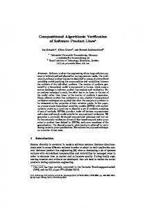
Figure 3: FTS of the vending machine. features in a single diagram. Formally, FTS are defined as follows. Definition 3 (Abstract syntax of FTS). An FTS f ts is a tuple f ts = (S, Act, trans, I, AP, L, d, γ, >) where • (S, Act, trans, I, AP, L) is a TS, • d = (N, r, DE) is an FD, • γ : trans → N is a total function, labelling transitions with features, • > ⊆ trans×trans is a partial order, defining priorities between transitions. Transition priorities offer an intuitive way to model cases in which one feature overrides the behaviour of another. If a transition t labelled with feature f has priority over transition t0 labelled with feature f 0 , this means that products containing both f and f 0 only have transition t; they would have both transitions if there were no priority relation. The transition free of the FreeDrinks feature, for instance, has priority over pay (which belongs to the root feature, VendingMachine). The result is that pay will not appear in any product that contains the feature FreeDrinks, such as the one in Figure 1(d).3 A common modelling pattern is that the behaviour of a child feature (wrt. the FD) overrides the behaviour of its parents. Formally, we can use the decomposition relation DE of the FD (a directed graph), to induce the priority relation of the FTS.
FEATURED TRANSITION SYSTEMS
In order to model the behaviour of each product in the SPL concisely, we draw upon existing approaches [12, 18, 20, 24] that create a single parameterised model to be instantiated differently for each product of the SPL. However, in contrast to most approaches, we explicitly relate behaviours to their originating features, and do this at the level of individual transitions.
3.1
cancel/c
free/f
Definition 2. An FA (resp. BA) is a tuple (Q, Σ, δ, Q0 , F ) where Q is a set of states, Σ is the alphabet, δ ⊆ Q × Σ × Q the transition relation, Q0 ⊆ Q a set of initial states and F ⊆ Q a set of accepting states. An FA accepts finite words that reach an accepting state, and a BA accepts infinite words that visit accepting states infinitely often.
3.
4
return/c
Syntax
The syntax of FTS accounts for the fact that adding a feature to a system modifies the behaviour of this system. Consider the vending machine example. Figures 1(b,c and d) show the impact of adding features Tea, CancelPurchase and FreeDrinks, respectively, to a machine serving only soda. Tea adds two transitions (tea and serveTea); CancelPurchase also adds two transitions; and FreeDrinks replaces transitions pay and change by a single transition free as well as open/close by skip. In order to describe the effects of several features on a system concisely, our approach models a system that contains all features, as well as annotations that indicate which transitions of the model correspond to which feature. To be able to express cases in which a feature removes (rather than adds) transitions, we use a priority relation over alternative transitions.2 This leads us to define a featured TS as a TS in which each transition is labelled with a feature, and where a priority relation may be associated to transitions leaving the same state. The FTS for the vending machine example is given in Figure 3. The feature label of a transition is shown next to its action label, separated by a slash. In addition, the transitions are coloured in the same way as the features in Figure 2. Intuitively, the FTS captures the impact of all
The purpose of an FTS is to model the behaviour of the whole SPL. From the FTS, one can obtain the behaviour of one particular product through projection. Intuitively, the diagrams (a), (b), (c) and (d) of Figure 1 can be obtained by removing selected transitions from Figure 3. Formally, in order to obtain the behaviour of a particular product, one projects the FTS on the corresponding set of features, say p ∈ [[d]]F D . This transformation is entirely syntactical and consists in removing (i) all transitions linked to features that are not in p, and (ii) all transitions that are overridden by higher priority transitions. The result of the projection is an ordinary TS.
2 In essence, removing a transition corresponds to adding an alternative transition of higher priority.
3 Since state 2 and transition change become unreachable, they are omitted from the diagram.
Definition 4 α
(Priorities induced by FD). A tranβ
sition s → s1 labeled with f1 has priority over s → s2 labeled β α with f2 , written s → s1 > s → s2 , iff f2 is an ancestor of f1 in DE.
337
Definition 5 (Projection). The projection of an FTS f ts to a product p ∈ [[d]]F D , noted f ts |p , is the TS t = (S, Act, trans0 , I, AP, L) where ˘ trans0 = (s1 , α, s2 )|(s1 , α, s2 ) ∈ trans ∧ γ(s1 , α, s2 ) ∈ p ∧ @(s1 , α0 , s02 ) ∈ trans • γ(s1 , α0 , s02¯) ∈ p ∧ (s1 , α0 , s02 ) > (s1 , α, s2 ) .
semantics does not apply to FTS. In addition, we want our model checker to indicate the products for which a property does (or does not) hold. To explore the state space of an FTS, a proper execution model thus needs to keep track of products and respect transition priorities. Consequently, we define the FTS reachability relation R0 , to be constructed as the state space is explored. R0 ⊆ S × P(P(N )) is a set of couples (s, px) such that state s is reachable by the products in px. In particular, the initial states of the FTS are reachable for all products.
Note that the concept of parallel composition also exists for FTS. If the modelled SPL consists of several processes running in parallel, each process can be modelled as a separate FTS, all sharing the same underlying features and FD. The FTS of the system can then be obtained by composing these processes. For FTS, one can easily adapt the wellaccepted handshake communication model, whereby the execution of parallel processes is synchronised on transitions with shared actions and otherwise interleaved.
3.2
Definition 8. Initially reachable states of an FTS are ¯ 4 ˘ Init0 = (s, [[d]]F D ) | s ∈ I . Given a state s reachable by products in px, a transition α leaving s, say t = s → s0 , can be fired for all products if its feature is part of all products in px and if there is no higherα0
priority transition s → s00 that could also be fired. If these conditions hold, s0 is reachable by the same products in px. In case the conditions do not hold, the transition cannot be fired for all products, that is, s0 will only be reachable by a subset of px and we proceed as follows:
Semantics
Each TS obtained through projection describes the behaviour (see Definition 1) of a particular product of the SPL. The semantics of an FTS is thus the union of the behaviours of the projections on all valid products.
• If a higher-priority transition t0 could equally be fired, then t can only be fired for (and thus s0 is only reachable by) the products that do not contain the feature of t0 .
Definition 6
(Semantics of an FTS). [ [[f ts]]F T S = [[f ts |c ]]T S c∈[[d]]F D
• If the feature of t is part of some products in px only, it can only be fired for (and thus s0 is only reachable by) these products.
An important observation is that, except for trivial cases, the FTS semantics we just defined is not equal to the usual TS semantics (as given by Definition 1). Formally, there exists an FTS f ts for which [[f ts]]F T S 6= [[T S(f ts)]]T S , where T S(f ts) is the TS obtained by removing d, γ and > from f ts. The vending machine SPL is an example for such an FTS. Indeed, an execution e in which the vending machine would ask the first customer for a coin and offer a free drink to the next one would be part of [[T S(f ts)]]T S , since in the TS, the choice between pay and free is non-deterministic. Yet, the execution does not correspond to any of the machines in the SPL: these should either always offer free drinks or always require payment, hence e 6∈ [[f ts]]F T S . More generally, we have the following theorem. Theorem 7
• If none of the products contains the feature of t, it cannot be fired at all. This is formalised in the following definition. Definition 9. The successors of a state s ∈ S reachable by products in px ∈ P(P(N )) can be computed with the following operator 4
Pnost0 (s, px) = α (s0 , px0 ) | s → s0 ∈ trans ∧ ˘ α px0 = p ∈ px | γ(s → s0 ) ∈ p ∧ ¯o α0 α0 α {γ(s → s00 ) | s → s00 > s → s0 } ∩ p = ∅ .
(FTS semantics vs. TS semantics).
∀f ts
•
Let us illustrate this with the vending machine FTS of Figure 3. State 1 is an initial state, and thus reachable by all products. From there, the transition pay can only be fired by products containing the feature v (the label of pay), and not containing the feature f (the label of the higher-priority transition free). State 2 is thus reachable by these products only. From state 2, transition change can be fired for all products containing v, and so state 3 is reachable by the same products as state 2.
[[f ts]]F T S ⊆ [[T S(f ts)]]T S
This theorem illustrates that one cannot simply use classical model checking algorithms directly on an FTS to verify properties for the complete SPL. While this verification might be sound, it is not always complete: by ignoring priorities, it would find false positives. Definition 6 shows another problem that we have to face when model checking an FTS: the exponential blowup caused by considering all products of the SPL. This adds to the state-explosion problem that already exists in classical model checking. These considerations justify the need for an FTS-specific model checking algorithm, but before we get there, we need a more operational definition of the FTS semantics.
3.3
Recording the set of products would be too expensive. |N | The set of reachable states will be of size O(|S|.22 ). We propose a more concise representation for a set of products: to state which features the products must have (required features, rf ) and which they cannot have (excluded features, ef ). This symbolic data structure is defined as follows.
Reachability in FTS
Definition 10. A triple (s, rf, ef ) ∈ S × P(N ) × P(N ) is a symbolic encoding of a tuple (s, px) ∈ S ×P(P(N )) such
A model checker is meant to perform a search in the state space of the FTS and thus needs an execution model that is faithful to the FTS semantics. As we just showed, TS
4
that [[(s, rf, ef )]] = (s, {p ∈ [[d]]F D | rf ⊆ p ∧ ef ∩ p = ∅}).
338
4.1
The new, efficient reachability relation R is thus a set of triples (s, rf, ef ), where the initially reachable states (Init) and the successors (P ost) are defined as follows.
We first need to define what it means for an FTS to be a model of a temporal property. As stated in the following definition, an FTS satisfies a temporal property if all its projections satisfy the property.
Definition 11. In symbolic representation, the initially ¯ 4 ˘ reachable states of an FTS are Init = (s, ∅, ∅) | s ∈ I ; the successors of a state s ∈ S reachable by products containing features rf ⊆ N and not containing features ef ⊆ N are
Definition 14 (Satisfaction in FTS). An FTS f ts satisfies a (regular, or ω-regular) property φ, iff ∀p ∈ [[d]]F D
4
P ost(s, rf, ef ) = ˘ 0 (s , rf 0 , ef 0 ) |
•
f ts |p |= φ.
Extending the |= relation, we note this f ts |= φ.
α
s → s0 α ∧ rf 0 = rf ∪ {γ(s → s0 )} S α0 ∧ ef 0 = ef ∪ α0 00 α 0 γ(s → s00 ) s→s >s→s ¯ ∧ ef 0 ∩ rf 0 = ∅ .
The FTS model checking problem can now be formalised. Definition 15 (MC(fts, φ)). Given a property φ and an FTS f ts, M C(f ts, φ) returns true iff f ts |= φ. If f ts 6|= φ, it returns false, a counterexample e, and a non-empty set of products px ⊆ [[d]]F D such that ∀p ∈ px • f ts |p 6|= φ with e as counterexample.
It can easily be shown that the symbolic successor function is equivalent to its explicit counterpart, that is: Theorem 12. For any (s, rf, ef ),
The basic model checking scenario is analogous to classical model checking: just as the returned counterexample might be one out of many violating traces, the set of violating products is not necessarily complete. In case of a violation, it is therefore not possible to know whether there are products that do satisfy the property. This gives rise to an SPLspecific model checking problem: determine which products satisfy and which violate the property.
P ost0 ([[(s, rf, ef )]]) = [[P ost(s, rf, ef )]] where [[.]] is trivially extended to sets of triples. Using this representation, the size of the reachability relation will be O(|S|.2|N | .2|N | ). Since triples with rf ∩ ef 6= ∅ can be ignored, this shrinks to O(|S|.3|N | ), which is significantly smaller than what we had previously. Its size can be further reduced by exploiting the following property: if a state s is known to be reachable by products in px, then it is also reachable by the products in any subset of px. Formally, if (s, px) ∈ R0 and (s, px0 ) ∈ R0 with px0 ⊆ px, it is sufficient to only keep (s, px) in R0 . More generally, it is sufficient to keep the maximal elements (an antichain) of the partial order induced by the subset relation ⊆ over {px | (s, px) ∈ R0 } for each state s. In terms of the symbolic representation that we are using, an equivalent partial order can be defined as follows.
Definition 16 (ExtMC(fts, φ)). Given a property φ and an FTS f ts, ExtM C(f ts, φ) returns true iff f ts |= φ. If f ts 6|= φ, it returns false and a set c of couples (e, px) where e is a counterexample and px a non-empty set of products such that ∀p ∈ px • f ts |p 6|= φ. Furthermore, it holds that [ ∀p ∈ [[d]]F D • p 6∈ px =⇒ f ts |p |= φ. (e,px)∈c
The last condition of the above definition states that the list of counterexamples has to be exhaustive, i.e. all products that are not mentioned satisfy the property. The procedure thus implicitly returns a set of violating and a set of satisfying products. A further variation of these two scenarios is useful for SPLE: limiting the verification to a subset of the products of the SPL. Basically, both scenarios would take px ⊆ [[d]]F D , the set of products to verify, as an additional parameter. From there on, the definitions are analogous.
Definition 13. For a state s ∈ S and a set R ⊆ s × P(N ) × P(N ), the relation v is defined as a partial order 4
over R: (s, rf, ef ) v (s, rf 0 , ef 0 ) = (rf ⊇ rf 0 ) ∧ (ef ⊇ ef 0 ). With this optimisation, testing whether a state s is reachable by products in px cannot be done by just checking whether (s, px) ∈ R0 . Indeed, if the state s is reachable by a greater set of products px0 with px ⊆ px0 , only (s, px0 ) will be in R0 . One therefore has to check whether ∃(s0 , px0 ) ∈ R • s = s0 ∧ px ⊆ px0 . In the symbolic representation, for a state (s, rf, ef ), this boils down to checking whether ∃(s0 , rf 0 , ef 0 ) ∈ R • s = s0 ∧ (s, rf, ef ) v (s0 , rf 0 , ef 0 ).
4.
FTS model checking scenarios
4.2
Synchronous product
As stated in Section 2, we follow the approach of automatabased model checking [33], where regular and ω-regular properties are expressed by automata. In this case, model checking is equivalent to checking whether or not the synchronous product of the system with the automaton representing the negation of the property has an empty language. The synchronous product of an FTS and an automaton is similar to that of a TS and an automaton [4]. That is, it uses the state labelling (the atomic propositions) of the FTS, and not the transition labels (as the parallel composition does). The difference from the standard definition is that it has to preserve feature labels and priorities of the original FTS.
MODEL CHECKING FTS
Our objective is to verify regular and ω-regular properties in such a way that (a) if a property is satisfied by the FTS, then it is also satisfied by every product of the SPL, and (b) if a property is violated, the algorithm reports a counterexample (a trace that violates the property) as well as the products of the SPL that violate the property. This differs from classical model checking algorithms which, in case of a violation, just return the counterexample. In SPL model checking, information about the violating products is needed to help the engineer correct the model.
Definition 17 (Synchronous product). For an FTS f ts = (S, Act, trans, I, AP, L, d, γ, >) and an FA/BA a = (Q, P(AP ), δ, Q0 , F ), the synchronous product is an FTS f ts ⊗ a = (S × Q, Act, trans0 , I 0 , AP 0 , L0 , d, γ 0 , >0 ), where
339
• AP 0 = Q and L0 (s, q) = q, i.e. the new FTS is labeled with the states of the FA/BA, α
Input: An FTS f ts = (S, Act, trans, I, AP, L, d, γ, >), a set of accepting states F ⊆ AP , a flag break instructing to stop upon discovery of a bad state, a set of required (resp. excluded) features rf0 and ef0 to delimit the products to explore. Output: T rue if a state s with L(s) ∈ F was found and a set of quadruplets (state, set of required, set of excluded features, error trace) with the violations, otherwise f alse.
L(t)
α
• (s, q) →0 (t, p) iff s → t ∧ q → p, • I 0 = {(s0 , q) | s0 ∈ I ∧ ∃q0 ∈ Q0 • (q0 , L(s0 ), q) ∈ δ}, i.e. the initial states are those that can be reached from an initial state of the FA/BA, α ` ´ α • γ 0 (s, q) →0 (t, p) = γ(s → t), α0
α
α
α0
• (s, q) →0 (t, p) >0 (s, q) →0 (t0 , p0 ) iff s → t > s → t0 . Note that the synchronous product of an FTS f ts and an automaton a is an FTS f ts0 , not an automaton. Its language, though, can be defined in the same way as for FA/BA in Definition 2. The accepting states are the states that are labelled with an accepting state of a, {s ∈ S × Q|L0 (s) ∈ F } and the words are the executions e ∈ [[f ts0 ]]F T S .
4.3
Model checking regular safety properties
To prove that an FTS f ts satisfies a regular property φ, the latter is negated and transformed into an FA: F A(¬φ). F A(¬φ) is then composed with the FTS: f ts ⊗ F A(¬φ) yielding a new FTS f ts0 which has to be proven empty. Conversely, to prove that f ts violates φ is to prove that f ts0 has an accepting run. This boils down to checking whether an accepting state, a ‘bad’ state s with L0 (s) ∈ FF A(¬φ) , is reachable in f ts0 . This is accomplished with a search in the reachability relation R, as discussed in Section 3.3. The easiest way to do this is by computing a fixpoint: the reachable states are the initially reachable states and those that can be reached from them, i.e. the least fixpoint of the successor operator [6]. Definition 18. The symbolic reachability relation R ⊆ S × P(N ) × P(N ) for an FTS is defined as R = µX
•
Init ∪ P ost(X),
1 2 3
R ← {(s0 , rf0 , ef0 ) | s0 ∈ I} ; T race ← [] ; bad ← ∅ ;
4 5 6 7
while I 6= ∅ do Take s0 from I; I ← I \ {s0 }; push((s0 , rf0 , ef0 ), T race);
8 9 10 11 12 13
14 15 16 17 18 19 20 21 22 23 24
% reachable states % current trace % set of bad states
while T race 6= [] do (s, rf, ef ) ← top(T race); if L(s) ∈ F then bad ← bad ∪ {(s, rf, ef, T race)}; if break then return true, bad end 8 0 9