Jinjun Wang, Wei Xu, Shenghuo Zhu, Yihong Gong. NEC Laboratories America, Inc. Cupertino, CA 95014, USA. {jjwang,xw,zsh,ygong}@sv.nec-labs.com.
EFFICIENT VIDEO OBJECT SEGMENTATION BY GRAPH-CUT Jinjun Wang, Wei Xu, Shenghuo Zhu, Yihong Gong NEC Laboratories America, Inc. Cupertino, CA 95014, USA {jjwang,xw,zsh,ygong}@sv.nec-labs.com ABSTRACT Segmentation of video objects from background is a popular computer vision problem and has many important applications. Most existing methods are either computationally expensive or require manual initialization, static cameras, and/or rigid scenes. In a previous work, we proposed a joint spatio-temporal linear regression algorithm to automatically cluster the sparse edge/corner pixels in each video frame and obtain two motion models for the object and background respectively. To label the rest pixels for object segmentation, in this paper we propose to model the OF residual error, color intensity residual error and temporal label consistency features, as well as color/edge orientation consistency constrains, in a graph, and apply the Graph-Cut algorithm to minimize the energy of the graph to obtain an optimal segmentation of the two motion layers boundaries. Finally the object layer is identified from the two using simple heuristics. Experimental segmentation result with videos taken by webcams is promising. 1. INTRODUCTION Video object segmentation has a lot of important applications in mobile communication, video conference, compression, etc. Most existing approaches perform motion estimations from image sequences and cluster pixels or color segments into regions of coherent motions. Many approaches solve the problem by estimating the parametric motion models and the supporting regions [1]. There is also much work done to group pixels or segments into layers based on the affinity of local measurements. However, spatial or temporal clues alone are not sufficient because different objects/layers may share similar colors or motions. There have been research efforts that strive to combine spatial and temporal features for improved segmentations [2]. Most of these methods work on pixel or color segment level where the computation cost is huge. In our previous work [3], an efficient motion layer identification algorithm was proposed: First the edge/corner pixels of each frame were extracted as feature points, and the Optical Flow (OF) [4] of these points between neighboring frames were extracted. A Joint Spatio-Temporal Linear
Regression algorithm was proposed to cluster these sparse OF vectors over successive frames (5 in [3]) into two affine models. Once the two motion layers were identified for the sparse feature pixels, a corresponding dense motion layers was created by using the Markov Random Field (MRF) model to label the rest of the pixels into one of the two motion layers by color and edge orientation consistency. Finally, some heuristics were implored to classify the two layers as either object or background. In our MRF model, the Gibbis Sampling method was used for inference due to its computation advantage (O(mt) where m is the number of edges in the graph [5] and t is the number of iterations) over other popular methods such as Graph-Cut (O(mn2 ) where n is the number of nodes in the graph) or Belief Propagation. In our implementation, the MRF model had a pyramidal structure, and Gibbis sampling was used on the top level layer only. The solutions for the lower level layers were updated by deterministic greedy method. However, the solution of the bottom level layer MRF, which is the generated dense motion layer for our problem, does not necessarily converge to a Maximize a Posterior (MAP) solution. And hence the obtained segmentation usually gives unsatisfactory boundaries for certain sequences (Fig.1.a). In addition, with low-textured images, such an inference framework tends to cluster a large region of the image into a single motion layer (Fig.1.b).
(a)
(b)
Fig. 1. Some segmentation results by [3] (a) Unsatisfactory segmentation boundary; (b) Incorrect segmentation These limitations have motivated us to explore additional features and inference methods. In this paper, we proposed to apply temporal constrains and apply Graph-Cut to obtain an optimal segmentation. The remainder of the paper is organized as follows: Section 2 revisits our Joint Spatio-
Temporal Linear Regression algorithm [3] which finds two set of motion model parameters for each frame. Section ?? presents our inference framework to propagate labeling from sparse feature points to the rest pixels based on Graph-Cut. Section 4 lists some experimental results and discussed the future work. Concluding marks are draw in section 5. 2. JOINT SPATIO-TEMPORAL LINEAR REGRESSION For each video frame, the edge/corner pixels are detected and their OF are extracted using the method in [4]. To cluster these OF vectors into two affine motion models, we proposed a Joint Spatio-Temporal Linear Regression algorithm which operates in the following manner: Given a set of N sparse feature points (i.e., the edge/corner pixels) Xi = {xi , yi } and their OF values between neighboring frames ∆i = {δxi , δyi }, i = 1, . . . , N , a linear regression can achieve two affine models Al , l = 1, 2 that minimize the following error function: · ¸ 2 X X Xi E= k∆Xi − Al · k2 (1) 1 l=1 i∈{li =l}
where li is the motion layer label of pixel Xi . To achieve reliable and smooth motion layers, we extend the computation of Al between two frames to a few more frames so that we can exploit the temporal consistency. The temporal consistency means that if a feature point in frame k belongs to the object/background layer, then its corresponding point in frame k + 1 should also belong to the object/background layer, and vice versa. The error function over M successive frames can be expressed as: JE =
M X 2 X X k=2 l=1 lik =l
· k∆Xik − Alk ·
Xik 1
¸
(b)
Fig. 2. Segmentation process (a) The original image; (b) The sparse labeling. The white and black pixels belong to different layers, and the gray region is unknown points (Fig.2.b), the next step is to propagate the labeling to the rest pixels. This section introduces our selected temporal features and the graph-cut method to create the dense motion layers for object segmentation. 3.1. Feature Selection An image can be regarded as an undirected graph where each pixel Xi stands for a node and a neighboring system (e.g., 4-neighboring) represents the edge between nodes. Given a labeling L = {li |i = 1, . . . , N } of the graph, the energy of the graph is: E(L) = Ed (L) + Es (L)
(3)
where Ed (L) is called the data term which measures how appropriate it is to assign label li to each pixel Xi , i = 1, . . . , N , and Es (L) is called the smooth term which measures the dependence between pixel Xi and its neighbors. In our implementation, the data term Ed (L) in Eq.3 is the weighted sum of three penalty functions, Ed (L) =
k2
subjective to lik = ljk−1 if Xik 7→ Xjk−1 f or ∀i; k = 2, . . . , M
(a)
N X (ω1 D1 (li ) + ω2 D2 (li ) + ω3 D3 (li ))
(4)
i=1
(2)
where the third summation in Eq.2 sums up the regression residues for all the feature points Xik that belongs to motion layer l, and lik 7→ ljk−1 means that the two points are the corresponding feature points between frames k and k − 1. By joint linear regression, we can obtain 2 · (M − 1) affine motion models parameters {Alk |l = 1, 2; k = 2, . . . , M } and the labels of each feature point lik (Fig.2). M is set to 5 in our implementation. 3. DENSE MOTION LAYER CREATION USING GRAPH-CUT When the two set of affine motion model parameters are obtained for each frame as well as the label of each feature
1. D1 (li ) takes the normalized residual error of OF vector ∆Xi going through transform Ali as the penalty, · ¸ Xi D1 (li ) = k∆Xi − Ali · k2 (5) 1 Note that since the OF vectors is available only for edge/corner pixels, D1 is sparse. Hence for non-feature point, we set its penalty to 1 for both labels. 2. D2 (li ) measures the color similarity between pixel Xi and its back projection Xi−1 (li ) in the previous frame with regard to affine transform Ali , D2i (li ) = exp(−kcoli − coli−1 (Ali )k2 /σ 2 ) where
coli−1 (Ali )
is the color of
(6)
Xi−1 (Ali ),
Xi−1 (Ali ) = (1 − Ali ) ·
·
Xi 1
¸
(7)
3. D3 (li ) gives an arbitrary penalty 1/ − 1 to pixel Xi if the label li−1 (Ali ) of Xi−1 (Ali ) equals/unequals to li , ½ 1 li−1 (Ali ) == li D3 (li ) = (8) −1 li−1 (Ali ) 6= li
There are many methods proposed in literature to solve the Graph-Cut problem [6]. In our implementation, all the pyramidical layers of the graph are solved simultaneously as illustrated in Fig.3.b.
The smooth term Es (L) in Eq.3 plays an important for segmentation. It “smoothes” the segmentation by considering the dependency between neighboring pixels. In our implementation, Es (L) is a weighted sum of two functions: Es (L) =
N X X
(λ1 V1 (li , lj ) + λ2 V2 (li , lj ))
(9)
(a)
(b)
i=1 j∈N (i)
1. V1 (li , lj ) measures the color similarity between pixel Xi and Xj , X V1 (li , lj ) = δ(li 6= lj ) exp(−kcoli −colj k2 /σ 2 )
Fig. 3. Pyramidical graph and energy minimization (a) The pyramidical graph from Fig.2.b; (b) Solution by Graph-Cut
j∈N (i)
(10) 2. V2 (li , lj ) gives the penalty of assigning different labels to neighboring edge pixels with the same normal direction that is perpendicular to the line connecting the two pixels, X V2 (li , lj ) = δ(li 6= lj )ei ej kdij ×di kkdij ×dj k j∈N (i)
(11) where dij is the unit vector connecting from point i to point j, and x × y is the cross product between the vectors x and y.
3.3. Object motion layer identification The above processing segments a video frame into two motion layers. To identify the object layer from the other, we use the following heuristic based on our observation: The object layer is generally more compact than the background. Hence we compute the location variation for both the motion layers, and take the one with the smaller variation as the object layer. Fig.4 shows some final segmentation and object layer identification results by our algorithms.
3.2. Energy minimization via Graph-Cut To build the graph, we use a H level pyramidal structure (Fig.3.a) to avoid convergency to trivial local minimum. Every upper level layer is one quarter the size of the lower level layer. H is set to 4 in our current implementation. The selected neighboring system for node i at level h is as follows: N (i, h) = {{4 − neighbour of i}, ith neighbour in layer h − 1 if h > 1, ith neighbour in layer h + 1 if h < H
Fig. 4. Segmentation by Graph-Cut and object identification (a) The final segmentation of Fig.2; (b) The image that was unable to be segmented by our previous method [3] as shown in Fig.1.b
4. EXPERIMENTAL RESULTS
In addition, the weight between pixel Xi and its neighbor is proportional to the spatial relationship of the two nodes. Hence Eq.9 becomes N X X
(b)
(12)
|i = 1, . . . , N ; h = 1, . . . , H}
Es (L) =
(a)
2hj −hi (λ1 V1i,j (li , lj ) + λ2 V2i,j (li , lj ))
i=1 j∈N (i)
(13)
In the experiment we recorded 12 video sequences by webcam with different speaker color, speaker motion, background complexity, background motion and camera motion. These sequences last between 10 to 23 seconds with frame rate being 6 fps, 320x240 in resolution. We used the GraphCut library provided by Boykov et al. [6]. The system could process each frame in 2-3 seconds, which means that the
Seq. 1
Seq. 2
Seq. 3
Fig. 5. Segmentation results Top-row: results generated by our method in this paper; bottom-row: results by our previous method [3] computational cost is almost the same as that in our previous work [3]. All the 12 sequences were successfully segmented. Fig.5 shows some example frames from 3 sequences. The first row of each sequence in Fig.5 is generated by our proposed method in this paper, and the second row is generated by our previous method [3]. It can be seen that our method proposed in this paper gave better segmentation boundary (Fig.5, Seq. 1 and 2) and works fine with low textured image (Fig.5, Seq. 3). It is also noticed that, the segmentation boundary might not always follow the expected boundary of the speaker. This can be reduced be fine tuning the value of w1 ∼ w3 and λ1 ∼ λ2 in Eq.4 and Eq.13 for the certain sequence. Our future research includes that of how to find an optimal set of parameters by, e.g., learning based method.
5. CONCLUSION In this paper we proposed an efficient object segmentation method. Compared with many existing methods, our approach is fully automatic with low computational cost and accurate segmentation performance. This has obvious the importance for mobile communication, video conference, etc applications.
6. REFERENCES [1] P. Torr, R. Szeliski, and P. Anandan, “An integrated bayesian approach to layer extraction from image sequences,” PAMI, vol. 23, no. 3, pp. 297–303, 2001. [2] Q. Ke and T. Kanade, “A subspace approach to layer extraction,” Proc. of CVPR’01, pp. 255–262, 2001. [3] M. Han, W. Xu, and Y. Gong, “Video object segmentation by motionbased sequential feature clustering,” Proc of ACM MultiMedia’06, 2006. [4] B. Lucas and T. Kanade, “An iterative image registration technique with an application to stereo vision,” Proc. of IJCAI’81, pp. 674–679. 1981 [5] Y. Boykov and V. Kolmogorov, “An experimental comparison of min-cut/max-flow algorithms for energy minimization in vision,” PAMI, vol 26, no. 19, pp 11241137, 2004. [6] Yuri Boykov, Olga Veksler, and Ramin Zabih, “Fast approximate energy minimization via graph cuts,” PAMI, vol. 23, no. 11, pp. 1222–1240, 2001.