1
Efficient XML Tree Pattern Query Evaluation using a Novel One-Phase Holistic Twig Join Scheme Zhewei Jiang1 Cheng Luo2 Wen-Chi Hou1 Dunren Che1 Qiang Zhu3
[email protected] [email protected] [email protected] [email protected] [email protected] 1
2
Department of Computer Science, Southern Illinois University, Carbondale, IL 62901 Department of Mathematics and Computer Science, Coppin State University, Baltimore, MD 21216 3 Department of Computer and Information Science in University of Michigan-Dearborn, Dearborn, MI 48128
Paper type Research paper Key words XML databases, query evaluation, Twig query evaluation
Abstract Purpose of this paper This paper aims to provide an efficient algorithm for XML twig query evaluation. Design/Methodology/Approach In this chapter, we propose a single-phase holistic twig pattern matching method based on the TwigStack algorithm. Our method applies a novel stack structure to preserve the holisticity of the twig matches. Twig matches rooted at elements that are currently in the root stack are output directly. Findings Without generating individual path matches as intermediate results, our method is able to avoid the storage and output/input of the individual path matches, and totally eliminate the potentially time-consuming merging operation. Experimental results demonstrate the applicability and advantages of our approach. What is original/value of paper Our paper proposes an efficient XML twig query evaluation algorithm, which by both theoretical analyses and empirical studies demonstrates its advantages over the current state-of-the-art algorithm TwigStack.
2
1 Introduction XML has become a widely accepted standard for data exchange and integration over the Internet. With the rapid growing popularity of the XML data and its applications, the demand for efficient query processing over XML documents is ever increasing. The problem of querying XML documents has become a major issue in database research. XML documents are often modeled as ordered trees and the relationships between elements are defined by nested structures. An XML query is typically specified as a pattern that selects subsets of elements satisfying certain structural relationships. Based on different structures, the patterns can be categorized as linear paths or twig patterns. The twig pattern, also called twig queries, describes a complex traversal of the document tree and retrieves document elements through a joint evaluation of multiple path expressions (Polyzotis 2004). For example, in XQuery language, the following statement: section // paragraph [figure AND table] searches for all the paragraphs that are nested inside sections and have at least one figure and one table. The core operation of XML query processing is to find all occurrences of the given patterns in the XML documents. In the past few years, the research for XML query processing mainly concentrates on designing the efficient structural indexes or numbering schemes. The structural indexes, such as DataGuide (Goldman 1997), 1-index (Milo 2004), and F&B index (Kaushik 2002), provide the structural information of the documents. By probing the structural indexes, one can traverse XML document more efficiently by avoiding scanning unnecessary search space. Approaches based on the numbering schemes usually encode the positional information of each element within the XML document. By applying these numbering schemes to a document, it is easy to determine the structural relationship between any two elements without traversing the entire document tree. By exploiting the advantageous property of numbering schemes, many approaches, such as stack-tree (Al-Khalifa 2002), TJFast (Lu 2005), Determined (Che 2008), PathStack and TwigStack (Bruno 2002), are developed to process path and twig queries.. Earlier numbering scheme based approaches (Al-Khalifa 2002; Florescu 1999; Shanmugasundaram 1999; Zhang 2001) typically first decompose a twig pattern into a set of binary patterns and then search for matches for these individual binary pattern. Finally, these matches are stitched together to form the answers to the twig query. Such decomposition-based algorithms generally have a drawback that they could generate a large number of intermediate binary pattern matches even though the input and final result size are much more manageable. Aiming at such a problem, Bruno et al. (2002) proposes the TwigStack algorithm, which generates only individual path matches that are sure to contribute to the final results for the ancestor-descendent type of queries. Like other approaches, it is a two-phase method in which individual path matches are generated in the first phase and then combined together (through a “merge-join” operation) to generate the final twig matches in the second phase. It is proved to be I/O and CPU optimal for the ancestor-descendent type of twig queries. Recently, many algorithms have been proposed to ameliorate the sub-optimality problem of the TwigStack for parent-child type of query. However, we observe that the overhead incurred by the two-phase nature of the “holistic family” of twig join algorithms including TwigStack represents an even worse deficiency (worse than the suboptimality) because the cost to output and then input the individual path matches, and then to merge them together to form the twig matches can be substantial, especially when there are a large number of matching paths in the document. To address this problem, we propose a new holistic one-phase twig join algorithm, which outputs the twig matches in their entireties without the need for a later merge operation. The new algorithm yields no intermediate results (to be output and then input), which eliminates significant amounts of time and space overheads. Instead of outputting individual path matches as soon as they are available, our method holds them until complete twig matches rooted at elements that are currently in the root stack are formed. We have conducted extensive experiments. The results show that our algorithm runs much faster and requires less memory than Twigstack.
3 The rest of the chapter is organized as follows. Section 2 introduces the background of XML query processing and gives a brief survey of the techniques used in twig join processing. Section 3 details our holistic one-phase twig join algorithm. In section 4, we present the experimental results. Section 5 concludes our discussion in this chapter.
2 Backgrounds 2.1 Data Model and Twig Queries An XML document is generally modelled as a node-labelled, ordered tree T = (VT, ET), where VT is the set of vertices in the tree and ET the set of edges. Each node v∈VT corresponds to an element or an attribute in the document. Each node is assigned a unique label, which represents the semantics of the element. Each edge e = (u,v)∈ET represents a directed element-subelement or element-attribute relationship between nodes u and v. If there is a directed edge from u to v, u is said to be a parent of v; if v is reachable from u via directed edges, u is said to be an ancestor of v. Region code has been adopted in much of the XML research (Al-Khalifa 2002; Bruno 2002; Jiang 2003; Zhang 2001). In this scheme, each node in the tree is assigned a label or index of a unique 3-ary tuple: (leftPos, rightPos, LevelNo), which represents the left, right positions, and level number of the node, respectively. The encoding is essentially accomplished by preorder traversal of the tree. The codes can be used to help determine the structure relationships between nodes in the tree. For example, node v is the descendent of node u, if and only if u.leftPos < v.leftPos < v.rightPos < u.rightPos. Furthermore, if u.LevelNo = v.LevelNo-1, then v is the child of u. XML queries can be classified into two classes: a simple (linear) path query and a twig (pattern) query. A simple path query is defined as a path expression (Krishnamurthy 2003), while a twig query specifies patterns of selection predicates on multiple elements that must hold the specified structural relationships. Formally speaking, given a twig query pattern Q and an XML document D, a match of Q in D is identified by a mapping from nodes in Q to nodes in D such that: (i) query node predicates are satisfied by the corresponding database nodes; (ii) the structural relationships between query nodes are satisfied by the corresponding database nodes. The answer to query Q with n nodes can be represented as a list of n-ary tuples, where each tuple (q1, q2, …, qn) consists of database elements that identify a distinct match of Q in D (Bruno 2002). Twig queries represent the most common and general form of traversal over XML documents. Figure 2.1 shows an example of an XML data tree and a twig query. The twig query is to find all the occurrences of 3-ary tupe (section, title, figure) in the document tree such that the section has a title and a figure. For easy description of the structure of a query, we shall define some terms. Consider the twig query in Figure 2.1 (b) as an example. In order to distinguish the nodes in a document tree and a query pattern, we call the nodes in a query pattern as a pattern node, a query node, or simply a node, while a data node in the document (or database) an element. To further differentiate nodes in a query, we will also call the pattern node "section" the root node of the query, and "title" and "figure" nodes the child nodes of "section" not matter whether the edges are / or // in the twig query. The nodes "title" and "figure" are called the leaf nodes of the query since no child node exists under them. For simplicity, elements that have the same tag name as the root node of the query in the document will be called root elements as far as a twig or path match is concerned. For example, the section element whose title is “Query” in the data tree is referred to as a root element. Accordingly, elements that have the same tag names as the leaf nodes of the query are referred to as leaf elements. For example, the title element named “Query” in Figure 2.1(a) is called a leaf element.
4
Figure 2.1 An XML Data Tree and a Twig Query Pattern
2.2 Twig Query Evaluation Algorithms There have been many algorithms developed for evaluating queries over XML data. Earlier approaches (Al-Khalifa 2002; Florescu 1999; Shanmugasundaram 1999; Zhang 2001) typically decompose a twig pattern into a set of binary (parent-child or ancestor-descendent) patterns and then search for matches to individual binary patterns in the document. Finally, the individual pattern matches are stitched together to form the answer to the entire twig query. These binary structural-join based algorithms generally have a drawback that they could generate very large (unused) intermediate results from the individual binary pattern matches even though the input and final result sizes are much more manageable. Aiming at such a problem, Bruno et al. (2002) proposes the PathStack algorithm. The algorithm processes an entire path, which includes a sequence of individual binary patterns, as a whole. It significantly reduces the size of the intermediate results generated by the structural join based algorithms. Noticing that PathStack can generate individual path matches that do not contribute to the final results of a twig query when it is applied directly to twig pattern evaluation, Bruno et al. (2002) therefore proposes the TwigStack algorithm. It generates only individual path matches that are sure to contribute to the final results for the ancestor-descendent type of queries. Like previous approaches, individual path results are combined together (by a “merge-join” operation) at the end to generate the final matches. TwigStack is proved to be I/O and CPU optimal for the ancestor-descendent type of twig queries. TwigStack is suboptimal for queries with parent-child relationships because it can still generate intermediate path matches that do not contribute to the final results. Several algorithms, all based on the TwigStack algorithm, have been proposed to deal with this issue. TwigStackList (Lu 2004) applies a look-ahead technique to examine ahead a limited amount of elements to avoid generating useless intermediate results. iTwigjoin (Chen 2005) proposes two elements partitioning schemes, one based on the tag name and level number (as opposed to TwigStack’s tag name only), the other based on the prefix-path of elements. The partitioning schemes are used to help prune away elements that do not match the twig pattern. Both TwigStackList and iTwigjoin are shown to be able to generate fewer intermediate path matches that do not contribute to the final results for some types of parent-child query. However, optimality still can not be guaranteed for all kinds of twig queries. TJFast (Lu 2005) employs a different encoding scheme, called the extended Dewey code, to XML data. It associates root-to-node path information, encoded by their extended Dewey scheme, with each node. The path encoding makes path matching simpler and more efficient though it is still based on the basic logic of TwigStack algorithm. Although the extended Dewey code gives a concise representation of the paths, tremendous storage overhead can still be incurred, especially when the tree is deep, as it redundantly records the entire path from the root to the node in question for every node. Storing variable-sized nodes, due to the variable root-to-node path length, can also complicate the design of the algorithm.
5
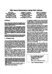
3. A One-Phase Holistic Twig Join Algorithm Extending the success of using stacks on containment joins and path queries, TwigStack has become the state-ofthe-art twig query evaluation algorithm. Many recently developed algorithms, such as TwigStackList, iTwigjoin, etc. (Chen 2005; Lu 2004) are all based on it. While much work (Chen 2005, Lu 2004) has focused on the suboptimality of the TwigStack for parent-child queries, we observe that other aspects of the algorithm can be more serious hindrances to the performance than the suboptimality. In this section, we describe our observations on the deficiencies of the TwigStack algorithm and present our solutions. 3.1 Observations on TwigStack Like most other algorithms in the holistic family, TwigStack is a two-phase algorithm, a path matching phase followed by a merge-joining phase. The two-phase algorithm requires the individual path matches, potentially large in number, be output at the end of the first phase, and then input and merged at the second phase. The output-and-theninput overhead of the found individual path matches (or the intermediate results) can be substantial if the number of intermediate path matches is large, and can be devastating if these matches cannot be held in memory. A single phase scheme can solve this problem elegantly. Merging paths to form twig matches in the second phase is simple, at least, conceptually, but it may turn out to be a very expensive process in reality. In TwigStack, path matches are output in group based on the path patterns and leaf elements. To merge these paths, an m-way merge is performed, where m is the number of different leaf elements in all the matching paths. Note that m can be very large, rendering this merge operation cumbersome and time consuming. In the following, we illustrate this issue by an example. Example. Merging Individual Path Matches. Consider the data tree and twig query in Figure 3.1.
Figure 3.1 Merging Path Matches
Assume each query node q is associated with a stack Sq. When c1 is pushed onto the stack SC in the TwigStack algorithm, showSolutionsWithBlocking() is called to output path match a1/c1 for the path pattern A//C. Later on, a1/d1 is output when d1 is encountered. Then, a1//d2 and a2/d2 are output when d2 is pushed onto stack SD. By the same token, a1//c2 and a2/c2 are output in the same batch, followed by a1//c3 and a2/c3 in another batch, then a1//c4 and a2/c4, and finally a1//d3 and a2/d3 are output. To merge these paths, a 7-way merge is performed for paths ending at c1, c2, c3, c4, d1, d2 and
6 d3, respectively. This can cause a serious problem when there are a large number of satisfying paths that end at different C and D nodes. A possible solution to this cumbersome merging is to first sort the matches based on the individual path patterns, i.e., A//C and A//D in the example, separately, and then perform now a 2-way merge. But sorting can also incur substantial overheads. We shall develop an algorithm that directly generates the final twig matches without complex merging or sorting. 3.2 Notations As in all the stack-based algorithms, there is a stream Tq associated with each pattern node q of the twig query. The stream contains the region codes for those elements that have the same node type as q. The elements in each stream are sorted by their leftPos. Some basic stream operation functions are: eof, advance, next, nextL and nextR, where eof tests the end of the stream, advance moves the cursor to the next element, next returns the next element in the stream, and nextL and nextR return leftPos and rightPos of the next element in the stream, respectively. The operations on stacks are: empty, pop, push, topL, topR. empty returns true when the stack is empty; pop and push, respectively, adds a new element to the stack and removes the top element from the stack. topL and topR return the leftPos and rightPos of the top element of the stack. Let e be an element in the document tree. We define ClosestPatternAncestor(e) as the closest ancestor of e in the document tree in terms of the query pattern. For example, in Figure 3.1, ClosestPatternAncestor(c2)= ClosestPatternAncestor(c3)= ClosestPatternAncestor(c4) = a2. We also define a pattern sibling element of e as an element in the document tree that (i) has the same node type as e; (ii) shares the same closest pattern ancestor with e, and (iii) does not have the ancestor-descendent relationship with e. For example, c4 is a pattern sibling element of c3 since they both share the same closest pattern ancestor a2 and they don’t have ancestor-descendent relationship. If d1 has another child c5, then c5 would have been a pattern sibling element of c1. Note that the definition of a pattern sibling element does not satisfy the normal definition of a “sibling” for a tree structure. 3.3 Stack Structure The overheads incurred in the TwigStack algorithm are caused by the “hasty” output of the individual path matches generated when a leaf element is encountered, which splits the twig matches as individual path matches. These individual path matches are at a later phase merged based on their root elements to form the twig matches. Here, the root elements refer to those elements that have the same node type as the root query node in the query pattern. In order to keep the holisticity of the twigs, we opt to delay the output of individual path matches by holding them in lists of stacks until all twig matches rooted at the top element of the root stack are formed. To hold the matching paths for the elements in the root stack, we associate each non-root query node with lists of stacks, in contract to the one stack per query node arrangement in TwigStack. Like other stack-based algorithms, an element is pushed onto a stack whose current top element is an ancestor of the incoming element. In addition, we require that the incoming element has the same closest pattern ancestor as the top element. For an element that does not satisfy the above conditions, it will be stored in a new stack. Elements that have the same closest pattern ancestor will be linked together for convenient access because they will be processed in the same way since they share the same closest pattern ancestor. In the following example, we give a more detailed description of the stack structure. Example. Stack structure. Figure 3.2 shows the stack state before outputting the twig matches for the document tree and twig pattern in Figure 3.1.
7
SD2
d3
d2
SD3
a2 a1
d1 SD1
SA
SC2
SC3
c3
c4
c2
c1 SC1
Figure 3.2 Stack Structure
In Figure 3.2, a1 is pushed onto the root stack SA first, followed by c1 onto SC1 and d1 onto SD1. SC1 and SD1 are each linked to a1, shown by the solid arrows in the figure, because a1 is the closest pattern ancestor for those elements in SC1 and SD1. Then, a2 is pushed onto the root stack SA as it is a descendent of a1. Later on, d2 is pushed onto a new stack SD2 because it has a different closest pattern ancestor (i.e., a2) than d1 (although d2 is a descendent of d1). SD2 is linked to a2 accordingly. When c2 is encountered, since it is not a descendent of c1, c2 is pushed onto a new stack, denoted by SC2. SC2 is linked to its closest pattern ancestor a2. c3 is pushed onto SC2 because it is a descendent of c2 and has the same closest pattern ancestor (i.e., a2) as c2. c4 is stored in a different stack SC3 because none of the top elements in the existing stacks of type C is an ancestor of c4. However, c4 does have the same closest pattern ancestor (i.e., a2) as elements in SC2. So, we link SC2 and SC3 together by using a dotted arrow pointing from c3 to its sibling element c4. Finally, d3 is placed in a new stack for the same reason as c4, and linked to element d2 in SD2 for having the same closest pattern ancestor as those elements in SD2. We have represented the closest pattern ancestor relationships (ClosestPatternAncestor()) by solid arrows in Figure 3.2, that is, a1 to SC1 and SD1, a2 to SC2 and SD2. It is observed that the commonly referenced ancestor-descendent relationships between query nodes, such as A//C and A//D, can be easily inferred from the closest pattern ancestor relationships by assuming that the ancestor elements of a stack “inherit” the relationships (i.e., the solid arrows) of their descendents (on the same stack). For example, we let a1 inherit the solid links of a2, that is, a1 implicitly has also links to SC2 and SD2 and thus the ancestor-descendent relationships (i.e., A//C, A//D) that a2 has with other type of elements. The twig matches for the elements in the root stack, e.g., a1 and a2, can be constructed easily by traversing the links following the query pattern. 3.4 Algorithm Our algorithm, named HolisticTwigStack, is presented in Figure 3.3. The algorithm computes the answer to a query twig pattern Q in one phase. We highlight the portions different from Twigstack in bold characters in the figure. Elements are checked for satisfaction of structural relationships in the same way as is done in TwigStack by recursively calling the function getNext(), which is defined in TwigStack. getNext(), returns a pattern node q_act such that the next element in the stream of q_act (i.e., next(Tq_act)) is guaranteed to find matching child/descendent elements to the twig pattern if it is a root element or its parent stack is not empty.
8 We attempt to withhold individual path matches rooted at the current elements of the root stack in memory. Like in TwigStack, an element is pushed onto a stack only if it is sure to contribute to a twig match. That is, if an element is a root element or its pattern parent element (which is an element that has the pattern parent node type of the incoming element and covers the incoming element) is already in the stack (line 03), then it is pushed onto stack (line 15), otherwise, we simply skip it (line 17). Before pushing an incoming element onto the stack, we need to further check whether it is beyond the range covered by the top element of the root stack (line 04). Only the top element needs to be checked because the forming of twig matches would complete sooner for elements at the top of the root stack than those at the bottom (because top elements cover only sub-ranges of what the bottom elements cover). If it falls in the range covered by the top root element and all the paths under the (top) root element are already formed (line 05), twig matches (rooted at the top root element) are output (line 06) and the root element is then removed from the stack (line 07). If the root stack still has other elements (line 08), the new top element will inherit the pointers (i.e., the solid links in Figure 3.1) of the previous top root element (line 09); otherwise, we clean all the child stacks (line 11). The same process (line 04line 14) will be repeated until the root stack is empty or the current root element can cover the incoming element. In HolisticTwigStack algorithm, the stack cleaning process is deferred until all twig matches, relevant to the current stack elements, have been output (line 11 and line 26) The element is pushed onto stack by calling the MoveElementToStack() procedure (line 15); otherwise, we discard it and advance to the next element (line 17). Since we use multiple lists of stacks to store different matching paths, it is a bit more complicated in our algorithm in pushing an element onto an appropriate stack. We shall explain the stack manipulation, i.e., MoveElementToStack() (in Figure 3.4) in detail later. After having reached the end of streams (end(Q)), we output the remaining twig matches related to the root elements left on stack Sroot (line 20 – line 27). Algorithm HolisticTwigStack(Q) 01 while not end(Q) 02 q_act=getNext(Q); 03
05 06 07 08 09 10 11 12 13 14
if (isRoot(q_act) || (at least one element in SParent(q_act) covers next (Tq_act)) while ((not Empty (Sroot) && (nextL(Tq_act) > topR(Sroot) ) if (no leaf stack is empty) ShowTwigSolution(Sroot, Sroot .size-1); Sroot.Pop(); if ( not Empty(Sroot)) Update the links between stacks; else Clean all child stacks; end if end if end while
15 16 17 18 19
MoveElementToStack(q_act); else advanceList(q_act); end if end while
04
20 while not empty(Sroot) 21 ShowTwigSolution(Sroot, Sroot .size-1); 22 Sroot.Pop(); 23 if ( not Empty(Sroot))
9 24 Update the links between stacks; 25 else 26 Clean all child stacks; 27 end while Figure 3.3 HolisticTwigStack Algorithm
Let us now explain how elements are pushed onto stacks and linked properly by the procedure MoveElementToStack(q_act) shown in Figure 3.4. Assume the stacks for a non-root pattern node q have been numbered in their order of creation as Sq1, Sq2, …, Sqn. For each incoming element of type q (i.e., Next(Tq)), we check if it is a descendent of the top element of the last stack Sqn and if it has the same closest pattern ancestor as the top element of the stack (line 04). (The correctness of only checking the last stack will be given as Lemma 3 in the next subsection.) If so, we push the element onto the stack Sqn (line 05); otherwise, we push the element onto a new stack Sqn+1 (line 07). In the latter case, we shall also check if it has the same closest pattern ancestor as any top element of a stack on an existing list since the top element and all the other elements in the same stack have the same closest pattern ancestor. If so, we append Sqn+1 to the end of that list by linking the incoming element to its sibling element (line 09). Otherwise, we directly link Sqn+1 to its closest pattern ancestor (line 11). Algorithm MoveElementToStack(q) 01 if (isRoot(q) 02 S_root.push(Next(Tq)) 03 04 05 06 07 08 09 10 11 12 13
else if (topR(Sqn) > nextL(Tq) and ClosetPatternAncestor(Next(Tq)) =ClosestPatternAncestor(top(Sqn)) push Next(Tq) into Sqn; else push Next(Tq) onto a new stack Sqn+1; if (ClosetPatternAncestor(Next(Tq)) = ClosestPatternAncestor(top(Sqi)) append Sqn+1 to the respective list; else link Sqn+1 to its ClosestPatternAncestor(Next(Tq)); end if end if Figure 3.4 MoveElementToStack algorithm
ShowTwigsolution() is called to output twig matches rooted at the current root element. The twig matches can be formed by following the solid and dotted links between stacks and the ancestor-descendent relationships between the elements in the same stacks. For simplicity, we shall not present the algorithm here but leave it to an appendix at the end of this chapter. Now we simply give an example as follows. Consider the stacks in Figure 3.2. The current (or top) root element is a2, which has two solid arrows to stacks SC2 and SD2, respectively. By following the links, both solid and dotted ones, we can reach SC2 and SC3 and their elements c2 , c3 and c4 . Similarly, d2 and d3 can be reached by following the links to SD3 and SD3. Thus, the twig matches rooted at a2 are (a2, c2 /c3 /c4 , d2/d3). After a2 is removed from the stack, a1 can then be processed. Recall that besides having its own reachable element c1, a1 inherits all a2 ‘s links (i.e., descendants, c2 /c3 /c4 and d2 /d3). As a result, the twig matches rooted at a1 are (a1, c1 /c2 /c3 /c4, d1 /d2/d3).
10 3.5 Analysis of Algorithm In this section, we show the correctness of the HolisticTwigStack algorithm and analyze its complexity. First, we introduce some terms and properties of TwigStack. Let subtreeNodes(q) be the set of pattern nodes, including q, in the subtree rooted at q in the query pattern Q. An element has a minimal descendent extension if there is a solution for the sub-query rooted at q, composed entirely of the head elements for subtreeNodes(q). Here, the head element of q, denoted as hq, is defined as the first element in Tq that participates in a solution for the sub-query rooted at q (Bruno 2002). TwigStack ensures that the element eq=next(Tq) is pushed onto the stack if and only if (i) element next(Tq) has a descendent element eqi in stream Tqi, for each qi∈children(q), and (ii) each of the element eqi recursively satisfies the first property (Bruno 2002). Lemma 1. Let e1, e2,…,em be the sequence of elements pushed onto the stacks during the execution of the algorithm. Then, e1.left < e2.left < …. < em.left. Proof: By Lemma 4.1 in (Bruno 2002), each time when getNext(Q) returns q, the current head element hq is guaranteed to have a descendent extension in subtreeNodes(q). If hq anticipates a final solution (and thus is pushed onto the stack), it must satisfy: (i)
Its left value is greater than any elements that are already in the stacks because any element in the ancestor of q that uses hq in a descendent extension is returned by getNext before q (Bruno 2002).
(ii)
Its left value is smaller than any elements that are still in the current streams because hq has the smallest left value than the current first element of any other stream Tq’, where q’ ∈ subtreeNodes(q’). This can be deduced from the fact that for each node q’ ∈ subtreeNodes(q’), the first element in Tq’ is hq’ (property 2 in Lemma 4.1 (Bruno 2002) )
Clearly, in any case, elements pushed onto the stacks later always have greater left values than elements pushed onto the stacks earlier. Lemma 2. The root element popped out of stack at line 07 and line 22 and elements deleted at line 11 and line 26 from the descendent stacks when the root stack is empty anticipate no further matches. So, the deletions are safe. Proof: [sketch] We already have nextL(Tq_act) > topR(Sroot) at line 04, and from Lemma 1, nextL(Tq_act) < nextL(Tq) for any q that is pushed onto the stacks after the current q_act. So, any element to be pushed onto a stack after the current nextL(Tq_act) cannot be covered by the current root element, which means all the descendents of the current root element have already been processed. It is safe to delete the current root element. Let us now show that once the root stack becomes empty, all elements in the descendent stacks can be removed safely. This is because later on if there is a new root element to be pushed onto the empty root stack, it must cover a disjointed range of the region codes than the previous popped out root elements. Thus, the descendents of the previous root element can be removed safely. # End of proof Earlier in the MoveElementToStack() procedure, when an element is to be pushed onto an appropriate stack, instead of examining all the stacks on the list we only check if it is a descendent of the top element of the last stack (of its type) and if it has the same closest pattern ancestor as the top element. This optimization is based on the following lemma.
11 Lemma 3: For each incoming element, either it can only be a descendent of the top element of the last stack (of its type), or it is not a descendent of any top element of the stacks (of its type). Proof: [sketch] In our algorithm, an element is pushed onto a new stack if it is not a descendent of the top elements of the existing stacks or it does not have the same closest pattern ancestor as the top element’s. In either case, the bottom element of a stack covers a disjointed range from all top elements of the preceding stacks. Consequently, all top elements of stacks have disjointed ranges. Notice that elements of the same type are sorted and processed in increasing order of their left position in their respective streams. Therefore, the incoming element whose left position is larger than the left position of the last stack’s top element, can only be the descendent of the top element of the last stack (and no others) or be pushed onto the new stack. So checking only the last stack is enough to guarantee the correctness of selecting an appropriate stack. # End of Proof Lemma 4: MoveElementToStack(q) correctly places the elements onto stacks and links non-root elements to their closest pattern ancestors. Proof: [sketch] We shall prove it by induction. (i) Basis. Let e1 be the first element in the stream Tq to be pushed onto the stack. MoveElementToStack(q) will create a new stack and link it to its ClosestPatternAncestor(). The structural relationship between the first element and its closest pattern ancestor is maintained correctly. (ii) Induction. Assume MoveElementToStack(q) correctly places subsequent elements e2, e3,…., en-1 into stacks and links them properly. For the next incoming element en, it is either pushed onto an existing stack or a new stack. If it is pushed onto an existing stack, by the rules of pushing elements onto stacks, it has the same closest pattern ancestor as its ancestor(s) who has been already linked correctly as assumed. If it is pushed onto a new stack, the new stack will either be directly linked to en’s closest pattern ancestor or appended to the stack list whose elements share the same closest pattern ancestor. It is obvious that the structural relationship between en and its closest pattern ancestor is maintained correctly in either case. # End of Proof Thus the elements in the stacks can be reached in any case as long as it participates the final match, which is guaranteed by the property of getNext(). The relevant proof can be found in (Bruno 2002). Theorem 1: Given a twig query pattern Q and an XML document tree D, Algorithm HolisticTwigStack correctly returns all answers to Q on D. Proof: [sketch] In HolisticTwigStack, we repeatedly find a pattern node q = getNext(Q) to process (line 02). Each incoming element next(Tq) is processed in the same way as in TwigStack except that the element is stored in a different stack structure by MoveElementToStack() for deferring output. The correctness of TwigStack has already been proved in (Bruno 2002). And Lemma 4 shows that MoveElementToStack() correctly maintain the twig structural relationships among elements in the stacks. Therefore, the steps from line 03 – line 18 guarantees that each incoming element is processed correctly. Once an element is in the stack, the only chances for it to be removed (after printing answers) before the end of the algorithm are at line 07, line 11, line 22 and line 26. We proved in Lemma 2 that both deletions are safe and would not affect any previous or subsequent query matching. The complete twig matches will be output at line 06 or line 21 and do not require any further merge operations.
12 # End of Proof Theorem 2: Given a twig pattern query Q, comprising of n nodes and only ancestor-descendent edges, over an XML document D, Algorithm HolisticTwigStack has the worst-case I/O and CPU time complexities linear in the sum of sizes of the n input lists and the output list. Furthermore, the worst-case space complexity of HolisticTwigStack is the sum of the sizes of the n input lists. Proof: Let N be the sum of the sizes of the n input lists (or the total size of input). For the I/O complexity, since we read n input lists and output the final result, it is linear in the sum of the size of input, i.e., N, and the output. As for the time complexity, HolisticTwigStack calls getNext() to examine every element in the input lists, it takes O(N) time. The time for pushing an element onto an appropriate stack is O(M), where M is the size of the longest input list, as we need to examine the stacks on a stack list to link the new element to its closest pattern ancestor. Thus, the entire stack manipulations takes O(NM). For the output part, we just need to follow the links to go through all the nodes in the stacks only once, it is O(N). So, overall time complexity is O(NM+N)=O(NM) in the worst case. For the space complexity, the stacks hold, in the worst case, all the n input lists. So, it is O(N). # End of Proof Let us make simple comparisons with TwigStack. Our algorithm may take a little more CPU time in stack manipulation, but TwigStack would require extra time and space to merge the individual path matches. In the worst case, the intermediate result size of TwigStack is O(K*P)=O(J), where K is the sum of the lengths of the input lists for all leaf nodes, and P is the length of the longest root-to-leaf path in the twig pattern. Since the intermediate result, i.e., the individual paths may not be sorted, in the worst case, it could require at least O(JlogJ) time to form the final twig matches by merging operations. It is important to note that our stacks store twig matches rooted at elements that are currently in the root stack, while TwigStack stores all the twig matches, in the form of individual path matches. Furthermore, nodes shared by multiple paths would have to be stored repeatedly in individual paths. Therefore, our algorithm in general uses much less space than TwigStack.
4. Experimental Results In this section, we present the results of experimental evaluations on the HolisticTwigStack algorithm. We compare its performance with TwigStack in terms of time and space utilizations on both synthetic and real-life data sets. 4.1 Experimental Setting We implemented the TwigStack and HolisticTwigStack algorithms in C++, and performed experiments on a modern computer with 3.4 GHz Pentium 4 CPU and 1GB RAM running the windows XP operating system. 4.2 Data Sets The following datasets are used for the experiments, which include both synthetic and real-world data. •
Random datasets
We implemented the random data generator in (Bruno 2002) to generate the datasets by three parameters: depth, fanout, and the number of different labels. In the experiments, the depth values vary from 5 to 10, fan-out from 2 to 10, and
13 the number of labels is chosen to be 7: A, B, C, D, E, F, and G, which are randomly distributed in the XML data trees. We generated roughly 500 such datasets for various experiments to measure the time and space usages of the algorithms. •
XMark
The XMark benchmark (Busse 2003) is a synthetic dataset generated based on an internet auction website database. The dataset used in our experiments is around 116 MB. It has 79 labels and 1,666,315 elements. We generate a region code file for each of the 79 labels. The total size of region code files is around 28 MB. •
DBLP
DBLP (University of Washington) is a real dataset that stores the computer science bibliography data. Each record represents a publication that contains up to 22 different fields, e.g., publisher, author, title, and so on. The dataset we chose has 3,332,130 elements, totalling 133 M bytes. We generated the region codes for each label based on the raw document tree. The sizes of the region code files representing different labels range from 1 K to 12,152 K bytes. The total size of all the 36 region code files is around 55.3 M bytes. 4.3 Twig Queries We selected twig queries with different characteristics to study the performance of the two algorithms. Figure 4.1 shows the twig queries run on the random datasets.
Figure 4.1. Twig Queries on Random Data Sets
Query Q1 represents a shallow and wide twig query; queries Q2 and Q3 represent deep twig queries with multiple branches. The queries chosen for XMark and DBLP datasets are based on the same idea. Figure 4.2 shows the twig queries for XMark. The twig queries used for DBLP are furnished as an appendix at the end of the chapter.
14
Figure 4.2 Twig Queries for XMark
4.4. Performance Metrics We measure the elapsed time in seconds and space requirements in bytes. A little explanation on the space usage and measurement is stated as follows. In TwigStack, individual path matches, or the intermediate results, need to be output and then input in its two phase processing. The intermediate results could have been stored on disks, but it would dramatically increase the total execution time. Therefore, we store them in memory, virtually eliminating the output and input cost of the intermediate results for TwigStack. The sizes of our random datasets have been intentionally set to small, e.g., 500 KB, so that the intermediate results of TwigStack can be held in memory. For TwigStack, each node on an individual path match is represented as a 2-tuple: (Type, Index), and thus needs 2 integers (8 bytes in Visual C++ complier) to store. The size of the stacks used in TwigStack is ignored because it is too small, compared to the size of intermediate results. As for the HolisticTwigStack, stack space makes up the most part of space requirements. It is used to hold twig matches rooted at elements currently in the root stack. Each node in a stack of HolisticTwigStack is represented by a 3tuple: (Type, Index, Pointer), where the pointer is used to link the node to another stacks, and thus requires 3 integers (12 bytes). For both methods, we measure the largest space requirement during the entire process of the query evaluation. 4.4. Experimental Results •
Random Datasets.
Figures 4.3 to 4.6 compare the performance of HolisticTwigStack with TwigStack on random datasets. Each result is the average of running a query over roughly 50 random datasets. The execution time of TwigStack has two parts: (i) time for finding individual path matches, shown as the lower parts of the bars in Figure 4.3, and (ii) time for merging paths, as the upper parts of the bars. As expected, HolisticTwigStack algorithm may spend a little more time on stack manipulation and forming the twig matches than the first phase of TwigStack, the costly merging phase determines the efficiency of the algorithm. The merging part makes up the most part of the cost for TwigStack. The entire execution time of TwigStack for Q1, Q2 and Q3 is 15, 2.5 and 15 seconds, while ours are 4, 1, 6 seconds, respectively. TwigStack’s are 3.8, 2.5 and 2.5 times longer than ours, respectively.
15 Execution Time (seconds)
16
M atching Phase of TwigStack M erge Phase of TwigStack HolisticStack
14 12 10 8 6 4 2 0 Q1
Q2 Queries on Random Data Set
Q3
Figure 4.3 Execution Time on Random Data Sets
Intermediate Result Size (bytes)
Figure 4.4 shows the space utilization. TwigStack uses 3,616, 30,496 and 71,440 bytes for queries Q1, Q2 and Q3, respectively, while ours uses only 1,464, 3,096 and 11,568 bytes for the same queries. Ours requires much less space than TwigStack. Indeed, this is well expected result because TwigStack needs to store all the twig matches in the form of individual path matches, while ours stores only the twig matches rooted at elements currently in the root stack, a subset of theirs. 71400 61400 51400
TwigStack HolisticTwigStack
41400 31400 21400 11400 1400 Q1 Q2 Queries on Random Data Set
Q3
Figure 4.4 Space Requirements for Random Data Sets The query result size is probably the most important factor that distinguishes the performance of the two algorithms. Note that if a query yields no match, then both algorithms would basically behave the same, that is, not pushing elements onto stacks (for ancestor-descendent type of queries) and no second phase for TwigStack. Therefore, we shall study how the result sizes affect the performance. Figures 4.5 and 4.6 illustrate the impacts of query result size on execution time and space requirement. We use the same set of parameters (fan-out, depth, and number of labels) to generate random datasets of the same size, here 20 KB with around 1,500 nodes. Although the datasets are small, it suffices to serve the purpose of showing the effect of query result size. The same query, here Q1 for illustration purpose, is posed to the datasets. Note that the results sizes of the query from these datasets are different. We present the results in Figures 4.5 and 4.6 in increasing order of the query result sizes. The result sizes range from 3,196,800 bytes (79,920 matches × 40 bytes/ match) to 31,702,720 bytes (792,568 matches × 40 bytes/ match). As shown in Figure 4.5, the larger the query results, the more time the algorithm require, especially for TwigStack. When the query result size is small, such as the case for Data1, both algorithms consume similar amount of time. But as the query result size increases, the difference becomes more evident. The execution time of TwigStack increases quickly from 2 seconds to 15 seconds as the query result size increases, while ours only increases from 1 to 4 seconds. The increases in the case of TwigStack are mainly due to the merging cost.
16 As explained earlier, TwigStack generally uses more space than ours. The differences in space usage become larger, in general, as the query result sizes increase. The space usages increase 1.7 times (from 840 to 1,464 bytes) for our method, slower than the 6.4 times (from 1,392 to 8,928) for TwigStack. In the figure, Data4 uses more space than Data5 to store the individual path matches but generates fewer query results. This is possibly because there are many elements of the same types under the same root elements in Data4, which would create a large number of twig match combinations.
Execution Time (seconds)
16 14 12
M atching Phase of TwigStack M erge Phase of TwigStack HolisticStack
10 8 6 4 2 0 Data1
Data2
Data3
Data4
Q1 on Random Data Sets
Data5
Intermediate Results Size (Bytes)
Figure 4.5 Execution Time for Q1 on Different Random Data Set
10000 9000 8000 7000 6000 5000 4000 3000 2000 1000 0
TwigStack HolisticTwigStack
Data1
Data2 Data3 Data4 Q1 on Random Data Sets
Data5
Figure 4.6 Space Requirements for Q1 on Different Random Data Set • XMark Similar results are observed from the experiments on XMark (Figure 4.7 and 4.8). Our algorithm runs 1.2 to 6 times faster than TwigStack for XMark data set (Figure 4.7). Again, this is due to the sizes of query results. TwigStack uses 2.0 to 1,882 times more space than ours for the XMark data set (Figure 4.8). Our method shows extraordinary edge in space utilization for Q3. We observe that the large ratio for Q3, i.e., 1,882, is caused by the uniform tree structure of XMark, which is explained as follows. In XMark, each person has one and only one Address and Profile fields and each address in turn has one and only one City and Country fields, each profile has one and only one Gender and Education fields. Because of the balanced structure, each root element has only six descendents (1 address, 1 profile, 1 city, 1 country, 1 gender, and 1 education). In HolisticTwigStack, the 6 descendent nodes will be pushed onto stacks immediately after the root element (Person) is pushed onto the root stack to complete the twig match. The twig match is outputted immediately. Thus, at any time, there are at most 7 nodes in the stacks. On the other hand, TwigStack needs to store 4 single path matches for each eligible root element, which takes 12 nodes. If there are n qualified root elements in the entire document tree, the total intermediate result will be 12n nodes, compared with 7 nodes of our method.
17
Execution Time (seconds)
7 6 5
Matching Phase of T wigStack Merge Phase of T wigStack HolisticStack
4 3 2 1 0 Q1
Q2
Q3
Queries on XM ark Data Set
Intermediate Result Size (Bytes)
Figure 4.7 Execution Time on XMark Data Set
160000
TwigStack HolisticTwigStack
140000 120000 100000 80000 60000 40000 20000 0
Q1 Q2 Q3 Queries On Xmark Data Set
Figure 4.8 Space Requirement for XMark Data Set • DBLP Similar results are observed in the experimental results on DBLP data set. Our algorithm runs 1.5 to 11 times faster than TwigStack (Figure 4.9). TwigStack method uses 1.3 to 2,332.8 times larger space than ours (Figure 4.10). Again, the reason that causes this huge difference in space utilization and execution time is the uniform and balanced tree structure of DBLP data set.
Matching Phase of T wigStack
Execution Time (seconds)
25
Merge Phase of T wigSt ack Holist icSt ack
20 15 10 5 0 Q1
Q2
Q3
Q4
Q5
Queries On DBLP Data Set
Figure 4.9 Execution Time on DBLP Data Set
Intermediate Result Size
18 TwigStack
180050 160050 140050 120050 100050 80050 60050 40050 20050 50
HolisticTwigStack
Q1
Q2
Q3
Q4
Queries on DBLP Data Set
Q5
Figure 4.10 Space Requirement for DBLP Data Set As a short summary, our algorithm generally runs faster and requires less memory than TwigStack. The larger the query result sizes, the better our algorithm performs, compared to TwigStack.
5. Conclusion In this chapter, we propose an efficient one-phase holistic twig pattern matching algorithm based on the TwigStack. Unlike TwigStack and other two-phase holistic twig join algorithms, our method eliminates the potentially expensive time and space overheads incurred in storing individual path matches and merging them into twig matches. We accomplish this goal by devising an efficient stack structure to hold matching paths until entire twig matches (for the elements currently in the root stack) are formed. Experimental results have confirmed that in comparison with TwigStack, our method is significantly more efficient in all tested cases. We believe this result can be generalized to all general cases, except for one special situation, i.e., when a twig query evaluates to an empty result set, and in this case our algorithm degenerates to TwigStack.
References Al-Khalifa, S., Jagadish, H. V., Koudas, N., Patel, J. M. Srivastava, D., & Wu, Y. (2002). Structural Joins: A Primitive for Efficient XML Query Pattern Matching . In Proceedings of IEEE ICDE Conference (pp. 141-152).
Bruno, N., Koudas, N., & Srivastava, D. (2002). Holistic Twig Joins: Optimal XML Pattern Matching. In Proceedings of ACM SIGMOD Conference (pp. 310-321). Che, D., Hou, W-C. (2008). Determined: a system with novel techniques for XML query optimization and evaluation. In
International Journal of Web Information Systems 4(1) (pp. 48-77) Chen, T., Lu, J., & Ling, T. W. (2005). On Boosting Holism in XML Twig Pattern Matching Using Structural Indexing Techniques. In Proceedings of ACM SIGMOD conference (pp. 455-466). Florescu, D., & Kossmann, D. (1999). Storing and querying XML data using an RDBMS. Bulletin of the Technical Committee on Data Engineering (pp. 27-34). Goldman, R., & Widom, J. (1997). DataGuides: Enabling Query Formulation and Optimization in Semistructured. In Proceedings of 23rd VLDB Conference (pp. 436-445). Jiang, H., Wang, W., Lu, H., & Yu, J.X. (2003). Holistic Twig Joins on Indexed XML Documents. In Proceedings of the 29th VLDB conference (pp. 310-321). Kaushik, R., Bohannon, P., Naughton, J. F., & Korth, H. F. (2002). Covering Indexes for Branching Path Queries. In Proceedings of the 2002 ACM SIGMOD Conference (pp. 133-144). Krishnamurthy, R., Kaushik, R., & Naughton, J. (2003). XML-to-SQL Query Translation Literature: The State of the Art and
19 st
Open Problems. In Proceedings of the 1 International XML Database Symposium (XSym) (pp. 1-18). Lu, J., Chen, T., & Ling, T. W. (2004). Efficient Processing of XML Twig Patterns with Parent Child Edges: A Look-ahead Approach. In Proceedings of CIKM (pp. 533-542). Lu, J., Ling, T. W., Chan, C.-Y., & Chen, T. (2005). From Region Encoding To Extended Dewey: On Efficient Processing of XML Twig Pattern, In Proceedings of the 31st VLDB conference (pp. 193-204). Milo, T., & Suciu, D. (1999). Index structures for path expressions. In Proceedings of the 7th International Conference on Database Theory (pp. 277–295). Polyzotis, N., Garofalakis, M., & Ioannidis, Y. (2004). Selectivity Estimation for XML Twigs. In Proceedings of IEEE ICDE Conference (pp. 264-275). Shanmugasundaram, J., Tufte, K., He, G., Zhang, C, DeWitt, D. & Naughton, J. F. (1999). Relational Databases for Querying XML Documents: Limitations and Opportunities. In Proceedings of VLDB Conference (pp. 302-314). Zhang, C., Naughton, J., DeWitt, D., Luo, Q., & Lohman, G. (2001). On Supporting Containment Queries in Relational Database Management Systems. In Proceedings of ACM SIGMOD Conference (pp. 425-436). Busse, R., Carey, M., Florescu, D., Kersten, M., Manolescu, I., Schmidt, A., & Waas, F. (2003). XMark – an XML Benchmark Project. http://monetdb.cwi.nl/xml/index.html University of Washington. XML Repository. http://www.cs.washington.edu/research/xmldatasets/
Appendix 1: Algorithm ShowTwigSolution Algorithm ShowTwigSolution(CurStack,int Pos) 01 MatchList=NULL; 02 CurNode=CurStack.at(Pos); 03 for each child ci of CurNode 04 if ci is leaf type 05 ChildList[i]=ShowLeafSolution(ci); 06 else 07 ChildList[i]=ShowTwigSolution(ci); 08 end for //deal with CurNode's sibling node 09 neighbour=false; 10 if (CurNode→Neighbour!=NULL) 11 NMatchList=ShowTwigSolution(CurNode’s Neigbour Stack, CurNode→Neighbour); 12 neighbour=true; 13 end if 14 Append NMatchList at the end of MatchList. //deal with CurNode's direct descendent node 15 if (Pos!=CurStack.size-1) 16 DMatchList=ShowSolution(CurStack, Pos); 17 for each childlist of CurNode’s descendent node 18 append it to CurNode’s child list of the same type 19 end if 20 Append DMatchList at the end of MatchList 21 Combine CurNode with its children together by all possible combinations 22 Append the combination results at the end of Matchlist
20 23 If (neighbour is true) 24 for each child list of CurNode’s neighbour node 25 append it to CurNode’s child list of the same type 26 end if 27 return MatchList; Algorithm ShowLeafSolution(CurNode) 01 LeafList=NULL; 02 Append CurNode at the end of LeafList 03 if CurNode’s direct descendent exists 04 ShowLeafSolution(CurNode’s direct descendent node) 05 if CurNode’neighbour exists 06 ShowLeafSolution(CurNode’s neighbour node) 07 return LeafList Child lists are used to store the child elements of the same kind under the current element. If the child is leaf node, we call ShowLeafSolution() to collect all the reachable leaf elements starting from the current leaf element; otherwise, ShowTwigSolution() needs to be recursively called to construct the child list. Note each child is a single path starting at the child node ci, not the single node. Take Q3 in Figure 4.1 as example, ShowTwigSolution(C) returns the list of single path “C//D//E”. After the child lists of the current element are constructed, its sibling element (if there is any) and its direct descendent element (if there is any) will be dealt with by calling ShowTwigSolution(). Here the direct descendent node is defined as the element that is on the top of the current node in the same stack and their positions’ difference is only 1. The result lists will be appended at the end of the match list. If the direct descendent node exists, its child lists also need to be appended to the child lists of current node according to their types. This is because, as we discussed before, the ancestor node inherit the descendent node’s relationships. After the child lists are finally constructed, current node and all the possible combinations of the children will be constructed at line 21, the matches rooted at the current node is finished and appended to the match list. Before return the match list, we need to append the neighbour’s child lists (if there is any) to CurNode’s child lists for future use. Because CurNode’s ancestor node also inherits CurNode’s neighbour’s relationship even though CurNode does not.
Appendix 2: Queries on DBLP Data Set