Efficiently Compiling Efficient Query Plans for Modern Hardware Thomas Neumann Technische Universitat ¨ Munchen ¨ Munich, Germany
[email protected] ABSTRACT As main memory grows, query performance is more and more determined by the raw CPU costs of query processing itself. The classical iterator style query processing technique is very simple and flexible, but shows poor performance on modern CPUs due to lack of locality and frequent instruction mispredictions. Several techniques like batch oriented processing or vectorized tuple processing have been proposed in the past to improve this situation, but even these techniques are frequently out-performed by hand-written execution plans. In this work we present a novel compilation strategy that translates a query into compact and efficient machine code using the LLVM compiler framework. By aiming at good code and data locality and predictable branch layout the resulting code frequently rivals the performance of handwritten C++ code. We integrated these techniques into the HyPer main memory database system and show that this results in excellent query performance while requiring only modest compilation time.
1.
Figure 1: Hand-written code vs. execution engines for TPC-H Query 1 (Figure 3 of [16]) CPUs. Third, this model often results in poor code locality and complex book-keeping. This can be seen by considering a simple table scan over a compressed relation. As the tuples must be produced one at a time, the table scan operator has to remember where in the compressed stream the current tuple is and jump to the corresponding decompression code when asked for the next tuple. These observations have led some modern systems to a departure from this pure iterator model, either internally (e.g., by internally decompressing a number of tuples at once and then only iterating over the decompressed data), or externally by producing more than one tuple during each next call [11] or even producing all tuples at once [1]. This blockoriented processing amortizes the costs of calling another operator over the large number of produced tuples, such that the invocation costs become negligible. However, it also eliminates a major strength of the iterator model, namely the ability to pipeline data. Pipelining means that an operator can pass data to its parent operator without copying or otherwise materializing the data. Selections, for example, are pipelining operators, as they only pass tuples around without modifying them. But also more complex operators like joins can be pipelined, at least on one of their input sides. When producing more than one tuple during a call this pure pipelining usually cannot be used any more, as the tuples have to be materialized somewhere to be accessible. This materialization has other advantages like allowing for vectorized operations [2], but in general the lack of pipelining is very unfortunate as it consumes more memory bandwidth. An interesting observation in this context is that a handwritten program clearly outperforms even very fast vectorized systems, as shown in Figure 1 (originally from [16]). In a way that is to be expected, of course, as a human might use tricks that database management systems would never come
INTRODUCTION
Most database systems translate a given query into an expression in a (physical) algebra, and then start evaluating this algebraic expression to produce the query result. The traditional way to execute these algebraic plans is the iterator model [8], sometimes also called Volcano-style processing [4]: Every physical algebraic operator conceptually produces a tuple stream from its input, and allows for iterating over this tuple stream by repeatedly calling the next function of the operator. This is a very nice and simple interface, and allows for easy combination of arbitrary operators, but it clearly comes from a time when query processing was dominated by I/O and CPU consumption was less important: First, the next function will be called for every single tuple produced as intermediate or final result, i.e., millions of times. Second, the call to next is usually a virtual call or a call via a function pointer. Consequently, the call is even more expensive than a regular call and degrades the branch prediction of modern Permission to make digital or hard copies of all or part of this work for personal or classroom use is granted without fee provided that copies are not made or distributed for profit or commercial advantage and that copies bear this notice and the full citation on the first page. To copy otherwise, to republish, to post on servers or to redistribute to lists, requires prior specific permission and/or a fee. Articles from this volume were invited to present their results at The 37th International Conference on Very Large Data Bases, August 29th - September 3rd 2011, Seattle, Washington. Proceedings of the VLDB Endowment, Vol. 4, No. 9 Copyright 2011 VLDB Endowment 2150-8097/11/06... $ 10.00.
539
up with. On the other hand the query in this figure is a simple aggregation query, and one would expect that there is only one reasonable way to evaluate this query. Therefore the existing query evaluation schemes seem to be clearly suboptimal. The algebraic operator model is very useful for reasoning over the query, but it is not necessarily a good idea to exhibit the operator structure during query processing itself. In this paper we therefore propose a query compilation strategy that differs from existing approaches in several important ways:
excellent performance, but, as shown in Figure 1, still does not reach the speed of hand-written code. Another way to improve query processing is to compile the query into some kind of executable format, instead of using interpreter structures. In [13] the authors proposed compiling the query logic into Java Bytecode, which allows for using the Java JVM. However this is relatively heavy weight, and they still use the iterator model, which limits the benefits. Recent work on the HIQUE system proposed compiling the query into C code using code templates for each operator [6]. HIQUE eliminates the iterator model by inlining result materialization inside the operator execution. However, contrary to our proposal, the operator boundaries are still clearly visible. Furthermore, the costs of compiling the generated C code are quite high [6]. Besides these more general approaches, many individual techniques have been proposed to speed up query processing. One important line of work is reducing the impact of branching, where [14] showed how to combine conjunctive predicates such that the trade-off between number of branches and number of evaluated predicates is optimal. Other work has looked at processing individual expressions more efficiently by using SIMD instructions [12, 15].
1. Processing is data centric and not operator centric. Data is processed such that we can keep it in CPU registers as long as possible. Operator boundaries are blurred to achieve this goal. 2. Data is not pulled by operators but pushed towards the operators. This results in much better code and data locality. 3. Queries are compiled into native machine code using the optimizing LLVM compiler framework [7]. The overall framework produces code that is very friendly to modern CPU architectures and, as a result, rivals the speed of hand-coded query execution plans. In some cases we can even outperform hand-written code, as using the LLVM assembly language allows for some tricks that are hard to do in a high-level programming language like C++. Furthermore, by using an established compiler framework, we benefit from future compiler, code optimization, and hardware improvements, whereas other approaches that integrate processing optimizations into the query engine itself will have to update their systems manually. We demonstrate the impact of these techniques by integrating them into the HyPer main-memory database management system [5] and performing various comparisons with other systems. The rest of this paper is structured as follows: We first discuss related work in Section 2. We then explain the overall architecture of our compilation framework in Section 3. The actual code generation for algebraic operators is discussed in more details in Section 4. We explain how different advanced processing techniques can be integrated into the framework in Section 5. We then show an extensive evaluation of our techniques in Section 6 and draw conclusions in Section 7.
2.
3. THE QUERY COMPILER 3.1 Query Processing Architecture We propose a very different architecture for query processing (and, accordingly, for query compilation). In order to maximize the query processing performance we have to make sure that we maximize data and code locality. To illustrate this point, we first give a definition of pipeline-breaker that is more restrictive than in standard database systems: An algebraic operator is a pipeline breaker for a given input side if it takes an incoming tuple out of the CPU registers. It is a full pipeline breaker if it materializes all incoming tuples from this side before continuing processing. This definition is slightly hand-waving, as a single tuple might already be too large to fit into the available CPU registers, but for now we pretend that we have a sufficient number of registers for all input attributes. We will look at this in more detail in Section 4. The main point is that we consider spilling data to memory as a pipeline-breaking operation. During query processing, all data should be kept in CPU registers as long as possible. Now the question is, how can we organize query processing such that the data can be kept in CPU registers as long as possible? The classical iterator model is clearly ill-suited for this, as tuples are passed via function calls to arbitrary functions – which always results in evicting the register contents. The block-oriented execution models have fewer passes across function boundaries, but they clearly also break the pipeline as they produce batches of tuples beyond register capacity. In fact any iterator-style processing paradigm that pulls data up from the input operators risks breaking the pipeline, as, by offering an iterator-base view, it has to offer a linearized access interface to the output of an arbitrarily complex relational operator. Sometimes operators could produce a certain small number of output tuples together cheaply, without need for copying. We therefore reverse the direction of data flow control. Instead of pulling tuples up, we push them towards the consumer operators. While pushing tuples, we continue pushing until we reach the next pipeline-breaker. As a consequence,
RELATED WORK
The classical iterator model for query evaluation was proposed quite early [8], and was made popular by the Volcano system [4]. Today, it is the most commonly used execution strategy, as it is flexible and quite simple. As long as query processing was dominated by disk I/O the iterator model worked fine. However, as the CPU consumption became an issue, some systems tried to reduce the high calling costs of the iterator model by passing blocks of tuples between operators [11]. This greatly reduces the number of function invocations, but causes additional materialization costs. Modern main-memory database systems look at the problem again, as for them CPU costs is a critical issue. The MonetDB system [1, 9] goes to the other extreme, and materializes all intermediate results, which eliminates the need to call an input operator repeatedly. Besides simplifying operator interaction, materialization has other advantages, too, but it also causes significant costs. The MonetDB/X100 system [1] (which evolved into VectorWise) selected a middle ground by passing large vectors of data and evaluating queries in a vectorized manner on each chunk. This offers
540
select from
initialize memory of Ba=b , Bc=z , and Γz for each tuple t in R1 if t.x = 7 materialize t in hash table of Ba=b for each tuple t in R2 if t.y = 3 aggregate t in hash table of Γz for each tuple t in Γz materialize t in hash table of Bz=c for each tuple t3 in R3 for each match t2 in Bz=c [t3 .c] for each match t1 in Ba=b [t3 .b] output t1 ◦ t2 ◦ t3
* R1,R3, (select R2.z,count(*) from R2 where R2.y=3 group by R2.z) R2 R1.x=7 and R1.a=R3.b and R2.z=R3.c Figure 2: Example Query
where
a=b
a=b
x=7
x=7
R1
z=c
z=c
R1
z;count(*)
tuples in CPU registers and only access memory to retrieve new tuples or to materialize their results. Furthermore, we have very good code locality as small code fragments are working on large amounts of data in tight loops. As such, we can expect to get very good performance from such an evaluation scheme. And indeed, as we will see in Section 6, such a query evaluation method greatly outperforms iteratorbased evaluation. The main challenge now is to translate a given algebraic execution plan into such code fragments. We will first discuss the high-level translation in the next section, and then explain the actual code generation in Section 4.
y=3
y=3
R2
Figure 4: Compiled query for Figure 3
z;count(*)
R3
R2
R3
original with pipeline boundaries Figure 3: Example Execution Plan for Figure 2 data is always pushed from one pipeline-breaker into another pipeline-breaker. Operators in-between leave the tuples in CPU registers and are therefore very cheap to compute. Furthermore, in a push-based architecture the complex control flow logic tends to be outside tight loops, which reduces register pressure. As the typical pipeline-breakers would have to materialize the tuples anyway, we produce execution plans that minimize the number of memory accesses. As an illustrational example consider the execution plan in Figure 3 (Γ denotes a group by operator). The corresponding SQL query is shown in Figure 2. It selects some tuples from R2 , groups them by z, joins the result with R3 , and joins that result with some tuples from R1 . In the classical operator model, the top-most join would produce tuples by first asking its left input for tuples repeatedly, placing each of them in a hash table, and then asking its right input for tuples and probing the hash table for each table. The input sides themselves would operate in a similar manner recursively. When looking at the data flow in this example more carefully, we see that in principle the tuples are always passed from one materialization point to another. The join a = b materializes the tuples from its left input in a hash table, and receives them from a materialized state (namely from the scan of R1 ). The selection in between pipelines the tuples and performs no materialization. These materialization points (i.e., pipeline boundaries) are shown on the right hand side of Figure 3. As we have to materialize the tuples anyway at some point, we therefore propose to compile the queries in a way that all pipelining operations are performed purely in CPU (i.e., without materialization), and the execution itself goes from one materialization point to another. The corresponding compilation for our running example is shown in Figure 4. (Note that we assume fully in-memory computation for now to keep the example readable.) Besides initialization, the code consists of four fragments that correspond to the pipeline fragments in the algebraic plan: The first fragment filters tuples from R1 and places them into the hashtable of Ba,b , the second does the same for R2 and Γz , and the third transfers the results from Γz into the hashtable of Bz=c . The fourth and final fragment passes the tuples of R3 along the join hash tables and produces the result. All four fragments in themselves are strongly pipelining, as they can keep their
3.2
Compiling Algebraic Expressions
When looking at the query code in Figure 4, we notice that the boundaries between operators are blurred. The first fragment for example combines the scan of R1 , the selection σx=7 , and the build part of Bc=z into one code fragment. The query execution code is no longer operator centric but data centric: Each code fragment performs all actions that can be done within one part of the execution pipeline, before materializing the result into the next pipeline breaker. The individual operator logic can, and most likely will, be spread out over multiple code fragments, which makes query compilation more difficult than usual. In addition, these code fragments have a very irregular structure. For example, for binary pipeline breakers materializing an input tuple from the left will be very different from materializing an input tuple from the right. In the iterator model everything is a simple next call, but here the complex operator logic directly affects the code generation. It is important to note that this is an advantage, not a limitation of the approach! The iterator model has a nice, simple interface, but it pays for this by using virtual function calls and frequent memory accesses. By exposing the operator structure, we can generate near optimal assembly code, as we generate exactly the instructions that are relevant for the given situation, and we can keep all relevant values in CPU registers. As we will see below, the abstractions that are needed to keep the code maintainable and understandable exist, i.e., all operators offer a uniform interface, but they exist only in the query compiler itself. The generated code exposes all the details (for efficiency reasons), but that is fine, as the code is generated anyway. From the point of view of the query compiler the operators offer an interface that is nearly as simple as in the iterator model. Conceptually each operator offers two functions: • produce() • consume(attributes,source)
541
B.produce B.consume(a,s)
B.left.produce; B.right.produce; if (s==B.left) print “materialize tuple in hash table”; else print “for each match in hashtable[” +a.joinattr+“]”; B.parent.consume(a+new attributes) σ.produce σ.input.produce σ.consume(a,s) print “if ”+σ.condition; σ.parent.consume(attr,σ) scan.produce print “for each tuple in relation” scan.parent.consume(attributes,scan) Figure 5: A simple translation scheme to illustrate the produce/consume interaction
+
C++
C+
C++ scan
Figure 6: Interaction of LLVM and C++ imented with generating C++ code from the query and passing it through a compiler at runtime, loading the result as shared library. Compiling to C++ was attractive as the C++ code could directly access the data structures and the code of our database system, which is also written in C++. However, it has several disadvantages. First, an optimizing C++ compiler is really slow, compiling a complex query could take multiple seconds. Second, C++ does not offer total control over the generated code, which can lead to suboptimal performance. In particular, overflow flags etc. are unavailable. Instead, we used the Low Level Virtual Machine (LLVM) compiler framework [7] to generate portable assembler code, which can then be executed directly using an optimizing JIT compiler provided by LLVM. While generating assembler code might sound daunting at first, producing assembler code using LLVM is much more robust than writing it manually. For example LLVM hides the problem of register allocation by offering an unbounded number of registers (albeit in Single Static Assignment form). We can therefore pretend that we have a CPU register available for every attribute in our tuple, which simplifies life considerably. And the LLVM assembler is portable across machine architectures, as only the LLVM JIT compiler translates the portable LLVM assembler into architecture dependent machine code. Furthermore, the LLVM assembler is strongly typed, which caught many bugs that were hidden in our original textual C++ code generation. And finally LLVM is a full strength optimizing compiler, which produces extremely fast machine code, and usually requires only a few milliseconds for query compilation, while C or C++ compilers would need seconds (see Section 6 and [6]). Still, one does not want to implement the complete query processing logic in LLVM assembler. First, because writing assembler code is more tedious than using a high-level language like C++, and second, because much of the database logic like index structures is written in C++ anyway. But one can easily mix LLVM and C++, as C++ methods can be called directly from LLVM and vice versa. (To the compiler, there is no difference between both types of code, as both result in native machine code and both have strongly typed prototypes.) This results in a mixed execution model which is metaphorically sketched in Figure 6. The complex part of the query processing (e.g., complex data structure management or spilling to disk) is written in C++, and forms the cogwheels in Figure 6. The different operators are connected together by LLVM code, which forms the chain in Figure 6. The C++ “cogwheels” are pre-compiled; only the LLVM “chain” for combining them is dynamically generated. Thereby we achieve very low query compilation times. In
Conceptually, the produce function asks the operator to produce its result tuples, which are then pushed towards the consuming operator by calling their consume functions. For our running example, the query would be executed by calling Ba=b .produce. This produce function would then in itself call σx=7 .produce to fill its hash table, and the σ operator would call R1 .produce to access the relation. R1 is a leaf in the operator tree, i.e., it can produce tuples on its own. Therefore it scans the relation R1 , and for each tuple loads the required attributes and calls σx=7 .consume(attributes, R1 ) to hand the tuple to the selection. The selection filters the tuples, and if it qualifies it passes it by calling Ba=b (attributes, σx=7 ). The join sees that it gets tuples from the left side, and thus stores them in the hash table. After all tuples from R1 are produced, the control flow goes back to the join, which will call Bc=z .produce to get the tuples from the probe side etc. However, this produce/consume interface is only a mental model. These functions do not exist explicitly, they are only used by the code generation. When compiling an SQL query, the query is first processed as usual, i.e., the query is parsed, translated into algebra, and the algebraic expression is optimized. Only then do we deviate from the standard scheme. The final algebraic plan is not translated into physical algebra that can be executed, but instead compiled into an imperative program. And only this compilation step uses the produce/consume interface internally to produce the required imperative code. This code generation model is illustrated in Figure 5. It shows a very simple translation scheme that converts B, σ, and scans into pseudo-code. The readers can convince themselves that applying the rules from Figure 5 to the operator tree in Figure 3 will produce the pseudo-code from Figure 4 (except for differences in variable names and memory initialization). The real translation code is significantly more complex, of course, as we have to keep track of the loaded attributes, the state of the operators involved, attribute dependencies in the case of correlated subqueries, etc., but in principle this simple mapping already shows how we can translate algebraic expressions into imperative code. We include a more detailed operator translation in Appendix A. As these code fragments always operate on certain pieces of data at a time, thus having very good locality, the resulting code proved to execute efficiently.
4. CODE GENERATION 4.1 Generating Machine Code So far we have only discussed the translation of algebraic expressions into pseudo-code, but in practice we want to compile the query into machine code. Initially we exper-
542
the concrete example, the complex part of the scan (e.g., locating data structures, figuring out what to scan next) is implemented in C++, and this C++ code “drives” the execution pipeline. But the tuple access itself and the further tuple processing (filtering, materialization in hash table) is implemented in LLVM assembler code. C++ code is called from time to time (like when allocating more memory), but interaction of the C++ parts is controlled by LLVM. If complex operators like sort are involved, control might go back fully into C++ at some point, but once the complex logic is over and tuples have to be processed in bulk, LLVM takes over again. For optimal performance it is important that the hot path, i.e., the code that is executed for 99% of the tuples, is pure LLVM. Calling C++ from time to time (e.g., when switching to a new page) is fine, the costs for that are negligible, but the bulk of the processing has to be done in LLVM. While staying in LLVM, we can keep the tuples in CPU registers all the time, which is about as fast as we can expect to be. When calling an external function all registers have to be spilled to memory, which is somewhat expensive. In absolute terms it is very cheap, of course, as the registers will be spilled on the stack, which is usually in cache, but if this is done millions of times it becomes noticeable.
4.2
data fragment (i.e., a sequence of tuples stored consecutively). The LLVM code first loads pointers to the columns that it wants to access during processing. Then, it loops over all tuples contained in the current fragment (code omitted). For each such tuple, it loads the attribute y into a register and checks the predicate. If the predicate is false, it continues looping. Otherwise, it loads the attribute z into a register and computes a hash value. Using this hash value, it looks up the corresponding hash entry (using the C++ data structures, which are visible in LLVM), and iterates over the entries (code omitted). If no matching group is found, it checks if it can assert sufficient free space to allocate a new group. If not, it calls into a C++ function that provides new memory and spills to disk as needed. This way, the hot code path remains purely within LLVM, and consists mainly of the code within the %then block plus the corresponding hash table iteration. Note that the LLVM call directly calls the native C++ method (using the mangled name @ ZN...), there is no additional wrapper. Thus, C++ and LLVM can interact directly with each other without performance penalty.
4.3
Performance Tuning
The LLVM code generated using the strategy sketched above is extremely fast. The main work is done in a tight loop over the tuples, which allows for good memory prefetching and accurate branch prediction. In fact the code is so fast that suddenly code fragments become a bottleneck that were relatively unimportant as long as the other code was slow. One prominent example is hashing. For TPC-H Query 1 (which is basically a single scan and a hash-based aggregation) for example more than 50% of the time of our initial plan was spent on hashing, even though we only hash two simple values. Another critical issue are branches. On modern CPUs, branches are very cheap as long as the branch prediction works, i.e., as long as the branches are taken either nearly never or nearly always. A branch that is taken with a probability of 50% however ruins the branch prediction and is very expensive. Therefore the query compiler must produce code that allows for good branch prediction. These issues require some care when generating assembly code. As mentioned before, we keep all tuple attributes in (virtual) CPU registers. For strings we keep the length and a pointer to the string itself in registers. In general we try to load attributes as late as possible, i.e., either in the moment that we need that attribute or when we get it for free anyway because we have to access the corresponding memory. Similar holds for computations of derived attributes. However when these values are needed on the critical path (e.g., when accessing a hash table using a hash value), it makes sense to compute these values a bit earlier than strictly necessary in order to hide the latency of the computation. Similarly, branches should be laid out such that they are amenable for ultra efficient CPU execution. For example the following (high-level) code fragment is not very prediction friendly:
Complex Operators
While code generation for scans and selections is more or less straightforward, some care is needed when generating code for more complex operators like sort or join. The first thing to keep in mind is that contrary to the simple examples seen so far in the paper it is not possible or even desirable to compile a complex query into a single function. This has multiple reasons. First, there is the pragmatic reason that the LLVM code will most likely call C++ code at some point that will take over the control flow. For example an external sorting operator will produce the initial runs with LLVM, but will probably control the merge phase from within C++, calling LLVM functions as needed. The second reason is that inlining the complete query logic into a single function can lead to an exponential growth in code. For example outer joins will call their consumers in two different situations, first when they have found a match, and second, when producing NULL values. One could directly include the consumer code in both cases, but then a cascade of outer joins would lead to an exponential growth in code. Therefore it makes sense to define functions within LLVM itself, that can then be called from places within the LLVM code. Again, one has to make sure that the hot path does not cross a function boundary. Thus a pipelining fragment of the algebraic expression should result in one compact LLVM code fragment. This need for multiple functions affects the way that we generate code. In particular, we have to keep track of all attributes and remember if they are currently available in registers. Materializing attributes in memory is a deliberate decision, similar to spooling tuples to disk. Of course not from a performance point of view, materializing in memory is relatively fast, but from a code point of view materialization is a very complex step that should be avoided if possible. Unfortunately the generated assembler code for real queries becomes complicated very quickly, which prevents us from showing a complete plan here, but as illustration we include a tiny LLVM fragment that shows the main machinery for the Γz;count(∗) (σy=3 (R2 )) part of our running example in Figure 7: The LLVM code is called by the C++ code for each
Entry* iter=hashTable[hash]; while (iter) { ... // inspect the entry iter=iter->next; } The problem is that the while mixes up two things, namely checking if an entry for this hash value exists at all, and checking if we reached the end of the collision list. The first
543
define internal void @scanConsumer(%8∗ %executionState, %Fragment R2∗ %data) { body: ... %columnPtr = getelementptr inbounds %Fragment R2∗ %data, i32 0, i32 0 %column = load i32∗∗ %columnPtr, align 8 1. locate tuples in memory %columnPtr2 = getelementptr inbounds %Fragment R2∗ %data, i32 0, i32 1 %column2 = load i32∗∗ %columnPtr2, align 8 2. loop over all tuples ... (loop over tuples , currently at %id, contains label %cont17) %yPtr = getelementptr i32∗ %column, i64 %id %y = load i32∗ %yPtr, align 4 3. filter y = 3 %cond = icmp eq i32 %y, 3 br i1 %cond, label %then, label %cont17 then: %zPtr = getelementptr i32∗ %column2, i64 %id 4. hash z %z = load i32∗ %zPtr, align 4 %hash = urem i32 %z, %hashTableSize %hashSlot = getelementptr %”HashGroupify::Entry”∗∗ %hashTable, i32 %hash %hashIter = load %”HashGroupify::Entry”∗∗ %hashSlot, align 8 %cond2 = icmp eq %”HashGroupify::Entry”∗ %hashIter, null 5. lookup in hash table (C++ data structure) br i1 %cond, label %loop20, label %else26 ... (check if the group already exists , starts with label %loop20) else26 : %cond3 = icmp le i32 %spaceRemaining, i32 8 6. not found, check space br i1 %cond, label %then28, label %else47 ... (create a new group, starts with label %then28) else47 : %ptr = call i8∗ @ ZN12HashGroupify15storeInputTupleEmj 7. full, call C++ to allocate mem or spill (%”HashGroupify”∗ %1, i32 hash, i32 8) ... (more loop logic) }
Figure 7: LLVM fragment for the first steps of the query Γz;count(∗) (σy=3 (R2 )) case will nearly always be true, as we expect the hash table to be filled, while the second case will nearly always be false, as our collision lists are very short. Therefore, the following code fragment is more prediction friendly:
we have to process tuples linearly, one tuple at a time. Our initial implementation pushes individual tuples, and this already performs very well, but more advanced processing techniques can be integrated very naturally in the general framework. We now look at several of them. Traditional block-wise processing [11] has the great disadvantage of creating additional memory accesses. However, processing more than one tuple at once is indeed a very good idea, as long as we can keep the whole block in registers. In particular when using SIMD registers this is often the case. Processing more than one tuple at a time has several advantages: First, of course, it allows for using SIMD instructions on modern CPUs [15], which can greatly speed up processing. Second, it can help delay branching, as predicates can be evaluated and combined without executing branches immediately [12, 14]. Strictly speaking the techniques from [14] are very useful already for individual tuples, but the effect can be even larger for blocks of tuples. This style of block processing where values are packed into a (large) register fits very naturally into our framework, as the operators always pass register values to their consumers. LLVM directly allows for modeling SIMD values as vector types, thus the impact on the overall code generation framework are relatively minor. SIMD instructions are a kind of inter-tuple parallelism, i.e., processing multiple tuples with one instruction. The second kind of parallelism relevant for modern CPUs is multicore processing. Nearly all database systems will exploit multi-core architectures for inter-query parallelism, but as the number of cores available on modern CPUs increases, intra-query parallelism becomes more important. In principle this is a well studied problem [10, 3], and is usually solved by partitioning the input of operators, processing each partition independently, and then merging the results from all partitions. For our code generation framework this
Entry* iter=hashTable[hash]; if (iter) do { ... // inspect the entry iter=iter->next; } while (iter); Of course our code uses LLVM branches and not C++ loops, but the same is true there, branch prediction improves significantly when producing code like this. And this code layout has a noticeable impact on query processing, in our experiments just changing the branch structure improved hash table lookups by more than 20%. All these issues complicate code generation, of course. But overall the effort required to avoid these pitfalls is not too severe. The LLVM code is generated anyway, and spending effort on the code generator once will pay off for all subsequent queries. The code generator is relatively compact. In our implementation the code generation for all algebraic operators required for SQL-92 consists of about 11,000 lines of code, which is not a lot.
5.
ADVANCED PARALLELIZATION TECHNIQUES
In the previous sections we have discussed how to compile queries into data-centric execution programs. By organizing the data flow and the control flow such that tuples are pushed directly from one pipeline breaker into another, and by keeping data in registers as long as possible, we get excellent data locality. However, this does not mean that
544
TPC-C [tps] total compile time [s]
HyPer + C++ 161,794 16.53
HyPer + LLVM 169,491 0.81
HyPer + C++ [ms] compile time [ms] HyPer + LLVM compile time [ms] VectorWise [ms] MonetDB [ms] DB X [ms]
Table 1: OLTP Performance of Different Engines kind of parallelism can be supported with nearly no code changes. As illustrated in Figure 7, the code always operates on fragments of data, that are processed in a tight loop, and materialized into the next pipeline breaker. Usually, the fragments are determined by the storage system, but they could as well come from a parallelizing decision. Only some additional logic would be required to merge the individual results. Note that the “parallelizing decision” in itself is a difficult problem! Spitting and merging data streams is expensive, and the optimizer has to be careful about introducing parallelism. This is beyond the scope of this paper. But for future work it is a very relevant problem, as the number of cores is increasing.
6.
Q2 374 2367 125 41 218 6555
Q3 141 1976 80 30 257 112 16410
Q4 203 2214 117 16 436 8168 3830
Q5 1416 2592 1105 34 1107 12028 15212
Table 2: OLAP Performance of Different Engines are shown in Table 1. As can be seen in the first row, the performance, measured in transactions per second, of the LLVM version is slightly better than performance of optimized C++ code. The difference is small, though, as most of the TPC-C transactions are relatively simple and touch less than 30 tuples. More interesting is the compile time, which covers all TPC-C scripts (in a PL/SQL style script language). Compiling the generated C++ code is more than a factor of ten slower than using LLVM, and results in (slightly) worse performance, which is a strong argument for our query compilation techniques. For the OLAP part, we ran the TPC-CH queries as prepared queries and measured the warm execution time. The results for the first five queries are shown in Table 2 (Q2 triggered a bug in VectorWise). DB X is clearly much slower than the other systems, but this is not surprising, as it was designed as a general purpose disk-based system (even though here the data fits into main memory and we measure warm execution times). The other systems are all much faster, but HyPer with the LLVM code generation is frequently another factor 2-4 faster, depending on the query. The comparison between the C++ backend and the LLVM backend is particularly interesting here. First, while the C++ version is reasonably fast, the compact code generated by the LLVM backend is significantly faster. This is less noticeable for Q5, which is dominated by joins, but for the other queries, in particular the aggregation query Q1, the differences are large. Q1 highlights this very well, as in principle the query is very simple, just one scan and an aggregation. The corresponding C++ code therefore looks very natural and efficient, but simply cannot compete with the LLVM version that tries to keep everything in registers. The second observation is that even though the queries are reasonably fast when crosscompiled into C++, the compile time itself is unacceptable, which was part of the reason why we looked at alternatives for generating C++ code. The compile time for the LLVM version however is reasonably modest (the numbers include all steps necessary for converting the SQL string into executable machine code, not only the LLVM code generation). Changing the backend therefore clearly payed off for HyPer, both due to query processing itself and due to compile times.
EVALUATION
We have implemented the techniques proposed in this paper both in the HyPer main-memory database management systems [5], and in a disk-based DBMS. We found that the techniques work excellent, both when operating purely in memory and when spooling to disk if needed. However it is difficult to precisely measure the impact our compilation techniques have relative to other approaches, as query performance is greatly affected by other effects like differences in storage systems, too. The evaluation is therefore split into two parts: We include a full systems comparison here, including an analysis of the generated code. A microbenchmark for specific operator behavior is included in Appendix B. In the system comparison we include experiments run on MonetDB 1.36.5, Ingres VectorWise 1.0, and a commercial database system we shall call DB X. All experiments were conducted on a Dual Intel X5570 Quad-Core-CPU with 64GB main memory, Red Hat Enterprise Linux 5.4. Our C++ code was compiled using gcc 4.5.2, and the machine code was produced using LLVM 2.8. The optimization levels are explained in more detail in Appendix C.
6.1
Q1 142 1556 35 16 98 72 4221
Systems Comparison
The HyPer system in which we integrated our query compilation techniques is designed as a hybrid OLTP and OLAP system, i.e., it can handle both kinds of workloads concurrently. We therefore used the TPC-CH benchmark from [5] for experiments. For the OLTP side it runs a TPC-C benchmark, and for the OLAP side it executes the 22 TPC-H queries adapted to the (slightly extended) TPC-C schema. The first five queries are included in Appendix D. As we are mainly interested in an evaluation of raw query processing speed here, we ran a setup without concurrency, i.e., we loaded 12 warehouses, and then executed the TPC-C transactions single-threaded and without client wait times. Similarly the OLAP queries are executed on the 12 warehouses single-threaded and without concurrent updates. What is interesting for the comparison is that HyPer originally compiled the queries into C++ code using hand-written code fragments, which allows us to estimate the impact LLVM has relative to C++ code. We ran the OLTP part only in HyPer, as the other systems were not designed for OLTP workloads. The results
6.2
Code Quality
Another interesting point is the quality of the generated LLVM code. As shown above the raw performance is obviously good, but it is interesting to see how the generated machine code performs regarding branching and cache effects. To study these effects, we ran all five queries using the callgrind tool of valgrind 3.6.0, which uses binary instrumentation to observe branches and cache effects. We used callgrind control to limit profiling to query processing itself. In the experiment we compared the LLVM version of HyPer with MonetDB. MonetDB performs operations in compact,
545
Q1 LLVM MonetDB branches 19,765,048 144,557,672 mispredicts 188,260 456,078 I1 misses 2,793 187,471 D1 misses 1,764,937 7,545,432 L2d misses 1,689,163 7,341,140 I refs 132 mil 1,184 mil
Q2 Q3 LLVM MonetDB LLVM MonetDB 37,409,113 114,584,910 14,362,660 127,944,656 6,581,223 3,891,827 696,839 1,884,185 1,778 146,305 791 386,561 10,068,857 6,610,366 2,341,531 7,557,629 7,539,400 4,012,969 1,420,628 5,947,845 313 mil 760 mil 208 mil 944 mil
Q4 Q5 LLVM MonetDB LLVM MonetDB 32,243,391 408,891,838 11,427,746 333,536,532 1,182,202 6,577,871 639 6,726,700 508 290,894 490 2,061,837 3,480,437 20,981,731 776,417 8,573,962 3,424,857 17,072,319 776,229 7,552,794 282 mil 3,140 mil 159 mil 2,089 mil
Table 3: Branching and Cache Locality
8.
tight loops, and can therefore be expected to have a low number of branch mispredictions. The results are shown in Table 3. The first block shows the number of branches, the number of branch mispredictions, and the number of level 1 instruction cache misses (I1). These numbers are indicators for the control flow and the code locality of the query code. Several things are noticeable. First, our generated LLVM code contains far less branches than the MonetDB code. This is not really surprising, as we try to generate all code up to the next pipeline breaker in one linear code fragment. Second, the number of branch mispredictions is significantly lower for the LLVM code. One exception is Q2, but this is basically a sub-optimal behavior of HyPer and not related to LLVM. (Currently HyPer is very pessimistic about spooling to disc, and copies strings around a lot, which causes more than 60% of the mispredictions. MonetDB avoids these copies). For all other queries the LLVM code has far less mispredictions than MonetDB. Interestingly the relative misprediction rate of MonetDB is quite good, as can be expected from the MonetDB architecture, but in total MonetDB executes far too many branches and thus has many mispredictions, too. The next block shows the caching behavior, namely the level 1 data cache misses (D1) and level 2 data misses (L2d). For most queries these two numbers are very similar, which means that if data is not in the level 1 cache it is probably not in the level 2 cache either. This is expected behavior for very large hash tables. Again the LLVM code shows a very good data locality and has less cache misses than MonetDB. As with branches, the string handling in Q2 degrades caching, but this will be fixed in future HyPer versions. For all other queries the LLVM code has far less cache misses than MonetDB, up to a factor of ten. The last block shows the number of executed instructions. These numbers roughly follow the absolute execution times from Table 2 and thus are not surprising. However, they show clearly that the generated LLVM code is much more compact than the MonetDB code. In a way that might stem from the architecture of MonetDB which always operates on Binary Association Tables (BATs), and thus has to touch tuples multiple times.
7.
REFERENCES
[1] P. A. Boncz, S. Manegold, and M. L. Kersten. Database architecture evolution: Mammals flourished long before dinosaurs became extinct. PVLDB, 2(2):1648–1653, 2009. [2] P. A. Boncz, M. Zukowski, and N. Nes. MonetDB/X100: Hyper-pipelining query execution. In CIDR, pages 225–237, 2005. [3] J. Cieslewicz and K. A. Ross. Adaptive aggregation on chip multiprocessors. In VLDB, pages 339–350, 2007. [4] G. Graefe and W. J. McKenna. The Volcano optimizer generator: Extensibility and efficient search. In ICDE, pages 209–218. IEEE Computer Society, 1993. [5] A. Kemper and T. Neumann. HyPer: A hybrid OLTP&OLAP main memory database system based on virtual memory snapshots. In ICDE, pages 195–206, 2011. [6] K. Krikellas, S. Viglas, and M. Cintra. Generating code for holistic query evaluation. In ICDE, pages 613–624, 2010. [7] C. Lattner and V. S. Adve. LLVM: A compilation framework for lifelong program analysis & transformation. In ACM International Symposium on Code Generation and Optimization (CGO), pages 75–88, 2004. [8] R. A. Lorie. XRM - an extended (n-ary) relational memory. IBM Research Report, G320-2096, 1974. [9] S. Manegold, P. A. Boncz, and M. L. Kersten. Optimizing database architecture for the new bottleneck: memory access. VLDB J., 9(3):231–246, 2000. [10] M. Mehta and D. J. DeWitt. Managing intra-operator parallelism in parallel database systems. In VLDB, pages 382–394, 1995. [11] S. Padmanabhan, T. Malkemus, R. C. Agarwal, and A. Jhingran. Block oriented processing of relational database operations in modern computer architectures. In ICDE, pages 567–574, 2001. [12] V. Raman, G. Swart, L. Qiao, F. Reiss, V. Dialani, D. Kossmann, I. Narang, and R. Sidle. Constant-time query processing. In ICDE, pages 60–69, 2008. [13] J. Rao, H. Pirahesh, C. Mohan, and G. M. Lohman. Compiled query execution engine using JVM. In ICDE, page 23, 2006. [14] K. A. Ross. Conjunctive selection conditions in main memory. In PODS, pages 109–120, 2002. [15] T. Willhalm, N. Popovici, Y. Boshmaf, H. Plattner, A. Zeier, and J. Schaffner. SIMD-scan: Ultra fast in-memory table scan using on-chip vector processing units. PVLDB, 2(1):385–394, 2009. [16] M. Zukowski, P. A. Boncz, N. Nes, and S. H´eman. MonetDB/X100 - a DBMS in the CPU cache. IEEE Data Eng. Bull., 28(2):17–22, 2005.
CONCLUSION
The experiments have shown that data-centric query processing is a very efficient query execution model. By compiling queries into machine code using the optimizing LLVM compiler, the DBMS can achieve a query processing efficiency that rivals hand-written C++ code. Our implementation of the compilation framework for compiling algebra into LLVM assembler is compact and maintainable. Thereforem the data-centric compilation approach is promising for all new database projects. By relying on mainstream compilation frameworks the DBMS automatically benefits from future compiler and processor improvements without re-engineering the query engine.
546
APPENDIX A.
void SelectTranslator::produce(CodeGen& codegen,Context& context) const { // Ask the input operator to produce tuples AddRequired addRequired(context,getCondition().getUsed()); input−>produce(codegen,context); }
OPERATOR TRANSLATION
Due to space constraints we could only give a high-level account of operator translation in Section 3, and include a more detailed discussion here. We concentrate on the operators Scan, Select, Project, Map, and HashJoin here, as these are sufficient to translate a wide class of queries. The first four operators are quite simple, and illustrate the basic produce/consume interaction, while the hash join is much more involved. The query compilation maintains quite a bit of infrastructure that is passed around during operator translation. The most important objects are codegen, which offers an interface to the LLVM code generation (operator-> is overloaded to access IRBuilder from LLVM), context, which keeps track of available attributes (both from input operators and, for correlated subqeueries, from “outside”), and getParent, which returns the parent operator. In addition, helper objects are used to automate LLVM code generation tasks. In particular Loop and If are used to automate control flow.
void SelectTranslator::consume(CodeGen& codegen,Context& context) const { // Evaluate the predicate ResultValue value=codegen.deriveValue(getCondition(),context); // Pass tuple to parent if the predicate is satisfied CodeGen::If checkCond(codegen,value); { getParent()−>consume(codegen,context); } }
Projection The (bag) projection is nearly a no-op, and is compiled away during operator translation, as it only informs its input about the required columns. The real effect occurs within the pipeline breakers, as they discard all columns that are not required. void ProjectTranslator::produce(CodeGen& codegen,Context& context) const { // Ask the input operator to produce tuples SetRequired setRequired(context,getOutput()); input−>produce(codegen,context); }
Scan
void ProjectTranslator::consume(CodeGen& codegen,Context& context) const { // No code required here, pass to parent getParent()−>consume(codegen,context); }
The scan uses the ScanConsumer helper class to access all relation fragments, accesses all tuples contained in the current fragment, registers the required columns as available upon demand (they will be cached by the context), and passes the tuple to the consuming operator. Note that, depending on the relation type, the ScanConsumer logic might create calls to C++ functions (e.g., page accesses) to access data fragments.
Map
void TableScanTranslator::produce(CodeGen& codegen,Context& context) const { // Access all relation fragments llvm::Value∗ dbPtr=codegen.getDatabasePointer(); llvm::Value∗ relationPtr=codegen.getPtr(dbPtr,db.layout.relations[table]); auto& required=scanConsumer.getPartitionPtr(); ScanConsumer scanConsumer(codegen,context) for (;db.relations[table]−>generateScan(codegen,relationPtr,scanConsumer);) { // Prepare accessing the current fragment llvm::Value∗ partitionPtr=required; ColumnAccess columnAccess(partitionPtr,required); // Loop over all tuples llvm::Value∗ tid=codegen.const64(0); llvm::Value∗ limit=codegen.load(partitionPtr,getLayout().size); Loop loop(codegen,codegen−>CreateICmpULT(tid,limit),{{tid,”tid”}}); { tid=loop.getLoopVar(0);
The map operator computes new columns by evaluating functions. Note that placement of computations, and ordering of maps and selections has already been done by the query optimizer. Therefore the translation is straight forward. void MapTranslator::produce(CodeGen& codegen,Context& context) const { // Figure out which columns have to be provided by the input operator IUSet required=context.getRequired(); for (auto iter=functions.begin(),limit=functions.end();iter!=limit;++iter) { (∗iter).function−>getUsed(required); required.erase((∗iter).result); } // Ask the input operator to produce tuples SetRequired setRequired(context,required); input−>produce(codegen,context); } void MapTranslator::consume(CodeGen& codegen,Context& context) const { // Offer new columns vector accessors; for (auto iter=functions.begin(),limit=functions.end();iter!=limit;++iter) accessors.push back(ExpressionAccess(codegen,∗(∗iter).function)); for (unsigned index=0,limit=accessors.size();indexconsume(codegen,context); ConsumerContext consumerContext(context); } unsigned slot=0; for (auto iter=required.begin(),limit=required.end();iter!=limit;++iter,++slot) consumerContext.registerIUProvider(&(getOutput()[∗iter].iu),&access[slot]);
Hash Join
// Push results to consuming operators getParent()−>consume(codegen,consumerContext);
The four operators shown above are relatively simple, as most of the logic is handled by pure LLVM code. A hash join is much more involved, as here control flow moves from LLVM into C++ and back. One could implement the hash join using only LLVM, of course, and for a pure main-memory hash join that is even reasonable. But if the hash join is expected to spool to disk if needed, it will have to call many methods that are query independent (for example I/O), and in our implementation these parts are written in C++. We first sketch the C++ code, as it defines the code template that is then augmented with LLVM fragments. The C++ code loads the build side into main memory, spooling to disk if needed. If data fits into main memory, it just joins
// Go to the next tuple tid=codegen−>CreateAdd(tid,codegen.const64(1)); loop.loopDone(codegen−>CreateICmpULT(tid,limit),{tid}); } } }
As a scan is a leaf operator, there is no consume part.
Selection For the selection the produce part is simple, it just adds the attributes required for the predicate to the context and calls its input operator. The consume part filters out all non-satisfying tuples.
547
with the probe side. Otherwise, it spools the probe side into partitions, too, and joins the partitions. For simplicity we limit ourselves to inner joins here, non-inner joins require additional bookkeeping to remember which tuples have been joined.
// Compute size and hash value llvm::Value∗ size=matHelperLeft.computeSize(codegen,materializedValues); llvm::Value∗ hash=matHelperLeft.computeHash(codegen,materializedValues); // Materialize in hash table, spools to disk if needed llvm::Value∗ ptr=codegen.callBase(HashJoinProxy::storeLeftInputTuple, {opPtr,size,hash}); matHelperLeft.materialize(codegen,ptr,materializedValues);
void HashJoin::Inner::produce() { // Read the build side initMem(); produceLeft(); if (inMem) { buildHashTable(); } else { // Spool remaining tuples to disk spoolLeft(); finishSpoolLeft(); }
// Right side } else { // Collect registers from the right side vector materializedValues; matHelperRight.collectValues(codegen,context,materializedValues); // Compute size and hash value llvm::Value∗ size=matHelperRight.computeSize(codegen,materializedValues); llvm::Value∗ hash=matHelperRight.computeHash(codegen,materializedValues); // Materialize in memory, spools to disk if needed, implicitly joins llvm::Value∗ ptr=codegen.callBase(HashJoinProxy::storeRightInputTuple, {opPtr,size}); matHelperRight.materialize(codegen,ptr,materializedValues); codegen.call(HashJoinInnerProxy::storeRightInputTupleDone,{opPtr,hash});
// Is a in−memory join possible? if (inMem) { produceRight(); return; }
} } void HJTranslatorInner::join(CodeGen& codegen,Context& context) const { llvm::Value∗ leftPtr=context.getLeftTuple(),∗rightPtr=context.getLeftTuple();
// No, spool the right hand side, too spoolRight(); // Grace hash join loadPartition(0); while (true) { // More tuples on the right? for (;rightScanRemaining;) { const void∗ rightTuple=nextRight(); for (LookupHash lookup(rightTuple);lookup;++lookup) { join(lookup.data(),rightTuple); } }
// Load into registers. Actual load may be delayed by optimizer vector leftValues,rightValues; matHelperLeft.dematerialize(codegen,leftPtr,leftValues,context); matHelperRight.dematerialize(codegen,rightPtr,rightValues,context); // Check the join condition, return false for mismatches llvm::BasicBlock∗ returnFalseBB=constructReturnFalseBB(codegen); MaterializationHelper::testValues(codegen,leftValues,rightValues, joinPredicateIs,returnFalseBB); for (auto iter=residuals.begin(),limit=residuals.end();iter!=limit;++iter) { ResultValue v=codegen.deriveValue(∗∗iter,context); CodeGen::If checkCondition(codegen,v,0,returnFalseBB); }
// Handle overflow in n:m case if (overflow) { loadPartitionLeft(); resetRightScan(); continue; }
// Found a match, propagate up getParent()−>consume(codegen,context); }
// Go to the next partition if ((++inMemPartition)>=partitionCount) { return; } else { loadPartition(inMemPartition); }
Example As a small, illustrational example, we show the generated LLVM code for the query
} }
select d_tax from warehouse, district where w_id=d_w_id and w_zip=’137411111’
Thus the LLVM code has to provide three functions: produce/consume as before, and an additional join function that the C++ code can call directly when joining tuples that had been spooled to disk. Note that in this case the hash table lookups etc. are already implemented in C++, so join is only called for likely join candidates. The produce function simply passes the control flow to the C++ code. The consume functions (one for each join side) hashes the join values, determines the relevant registers, and materializes them into the hash table. Note that for performance reasons the HyPer system skips the in-memory materialization of the right hand side and directly probes the hash table if no data was spooled to disk, but this was omitted here due to space constraints.
below. It first scans warehouse, filters, and materializes into the hash table. Then it scans district and joins. Note that we “forced” a pure main-memory hash join to keep the code size reasonable.
void HJTranslatorInner::produce(CodeGen& codegen,Context& context) const { // Construct functions that will be be called from the C++ code { AddRequired addRequired(context,getCondiution().getUsed().limitTo(left)); produceLeft=codegen.derivePlanFunction(left,context); } { AddRequired addRequired(context,getCondiution().getUsed().limitTo(right)); produceRight=codegen.derivePlanFunction(right,context); } // Call the C++ code codegen.call(HashJoinInnerProxy::produce.getFunction(codegen), {context.getOperator(this)}); } void HJTranslatorInner::consume(CodeGen& codegen,Context& context) const { llvm::Value∗ opPtr=context.getOperator(this);
define void @planStart(%14∗ %executionState) { body: %0 = getelementptr inbounds %14∗ %executionState, i64 0, i32 0, i32 1, i64 0 store i64 0, i64∗ %0, align 8 %1 = getelementptr inbounds %14∗ %executionState, i64 0, i32 1 call void @ ZN5hyper9HashTable5resetEv(%”hyper::HashTable”∗ %1) %2 = bitcast %14∗ %executionState to %”hyper::Database”∗∗ %3 = load %”hyper::Database”∗∗ %2, align 8 %4 = getelementptr inbounds %”hyper::Database”∗ %3, i64 0, i32 1 %5 = load i8∗∗ %4, align 8 %warehouse = getelementptr inbounds i8∗ %5, i64 5712 %6 = getelementptr inbounds i8∗ %5, i64 5784 %7 = bitcast i8∗ %6 to i32∗∗ %8 = load i32∗∗ %7, align 8 %9 = getelementptr inbounds i8∗ %5, i64 5832 %10 = bitcast i8∗ %9 to %3∗∗ %11 = load %3∗∗ %10, align 8 %12 = bitcast i8∗ %warehouse to i64∗ %size = load i64∗ %12, align 8 %13 = icmp eq i64 %size, 0 br i1 %13, label %scanDone, label %scanBody scanBody: %tid = phi i64 [ 0, %body ], [ %34, %cont2 ] %14 = getelementptr i32∗ %8, i64 %tid %w id = load i32∗ %14, align 4 %15 = getelementptr inbounds %3∗ %11, i64 %tid, i32 0 %16 = load i8∗ %15, align 1 %17 = icmp eq i8 %16, 9 br i1 %17, label %then, label %cont2 then: %w zip = getelementptr inbounds %3∗ %11, i64 %tid, i32 1, i64 0 %27 = call i32 @memcmp(i8∗ %w zip, i8∗ @”string 137411111”, i64 9) %28 = icmp eq i32 %27, 0 br i1 %28, label %then1, label %cont2
// Left side if (source==left) { // Collect registers from the left side vector materializedValues; matHelperLeft.collectValues(codegen,context,materializedValues);
then1: %29 = zext i32 %w id to i64
548
100 %30 = call i64 @llvm.x86.sse42.crc64.64(i64 0, i64 %29) %31 = shl i64 %30, 32 %32 = call i8∗ @ ZN5hyper9HashTable15storeInputTupleEmj(%”hyper:: HashTable”∗ %1, i64 %31, i32 4) %33 = bitcast i8∗ %32 to i32∗ store i32 %w id, i32∗ %33, align 1 br label %cont2
90
execution time [ms]
80
cont2: %34 = add i64 %tid, 1 %35 = icmp eq i64 %34, %size br i1 %35, label %cont2.scanDone crit edge, label %scanBody
70 60 50 40 30 20
cont2.scanDone crit edge: %.pre = load %”hyper::Database”∗∗ %2, align 8 %.phi.trans.insert = getelementptr inbounds %”hyper::Database”∗ %.pre, i64 0, i32 1 %.pre11 = load i8∗∗ %.phi.trans.insert, align 8 br label %scanDone
10 0 0
scanDone: %18 = phi i8∗ [ %.pre11, %cont2.scanDone crit edge ], [ %5, %body ] %district = getelementptr inbounds i8∗ %18, i64 1512 %19 = getelementptr inbounds i8∗ %18, i64 1592 %20 = bitcast i8∗ %19 to i32∗∗ %21 = load i32∗∗ %20, align 8 %22 = getelementptr inbounds i8∗ %18, i64 1648 %23 = bitcast i8∗ %22 to i64∗∗ %24 = load i64∗∗ %23, align 8 %25 = bitcast i8∗ %district to i64∗ %size8 = load i64∗ %25, align 8 %26 = icmp eq i64 %size8, 0 br i1 %26, label %scanDone6, label %scanBody5
1 2 number of filtered columns
3
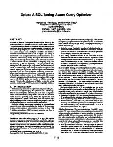
Figure 8: Performance for Cascading Selections uation schemes of modern cache-conscious database systems like MonetDB and VectorWise. We only considered the compiled model here, as both MonetDB and VectorWise use pre-compiled building blocks to reduce interpretation overhead. Note that during the experiments the data is held in a column-store layout, i.e., accessing more columns increases the amount of scanned data. As first experiment we started with a very simple aggregation query for our TPC-C data set
scanBody5: %tid9 = phi i64 [ 0, %scanDone ], [ %58, %loopDone ] %36 = getelementptr i32∗ %21, i64 %tid9 %d w id = load i32∗ %36, align 4 %37 = getelementptr i64∗ %24, i64 %tid9 %d tax = load i64∗ %37, align 8 %38 = zext i32 %d w id to i64 %39 = call i64 @llvm.x86.sse42.crc64.64(i64 0, i64 %38) %40 = shl i64 %39, 32 %41 = getelementptr inbounds %14∗ %executionState, i64 0, i32 1, i32 0 %42 = load %”hyper::HashTable::Entry”∗∗∗ %41, align 8 %43 = getelementptr inbounds %14∗ %executionState, i64 0, i32 1, i32 2 %44 = load i64∗ %43, align 8 %45 = lshr i64 %40, %44 %46 = getelementptr %”hyper::HashTable::Entry”∗∗ %42, i64 %45 %47 = load %”hyper::HashTable::Entry”∗∗ %46, align 8 %48 = icmp eq %”hyper::HashTable::Entry”∗ %47, null br i1 %48, label %loopDone, label %loop
select count(*) from orderline where ol_o_id>0 and ol_d_id>0 and ol_w_id>0 and varied the number of filter conditions, all of which are unselective (i.e., the result is the same for any combination of filter conditions). As we were interested in the overhead of data-passing, each filter condition was introduced as separate selection operator, and then measured the execution time of the query under the different evaluation schemes. The results are shown in Figure 8. Clearly, the iterator model using an interpreted predicate check (i.e., the evaluation scheme used in most database systems) is very slow. It performs a very large number of function calls and has poor locality. Compiling the iterator model into executable code greatly improves the runtime, in particular since the virtual function calls necessary for predicate evaluation are eliminated. Clearly, compiling into machine code is a good idea, interpreted approaches are significantly slower. The block-wise execution model improves execution times even more. Without filter, it is actually a bit slower, as the overhead of finding block boundaries, setting up tuple blocks frames, etc., does not pay off here. But even for a single selection the reduced number of function calls and better locality pays off, and it outperforms the iterator model. The data-centric approach proposed here shows excellent performance for all queries. Two points are particularly interesting: First, without filter conditions, the query execution time is nearly zero. The reason for this is that the compiler notices that our loop over tuple fragments performs no work except increasing a counter, and converts it into an addition of the fragment size. Second, when filtering (and thus accessing) all three columns, the performance seems to go down a bit. But in reality, the two-filter case is too fast due to caching effects. The three-filter query is reading tuple attributes at a rate of 4.2 GB/s, which starts getting close to the bandwidth of the memory bus of our machine, and branches depending on these data reads. We might improve query processing a bit by using conditional CPU operations, but with generic selection code we cannot expect to get much faster.
loopStep: %49 = getelementptr inbounds %”hyper::HashTable::Entry”∗ %iter, i64 0, i32 1 %50 = load %”hyper::HashTable::Entry”∗∗ %49, align 8 %51 = icmp eq %”hyper::HashTable::Entry”∗ %50, null br i1 %51, label %loopDone, label %loop loop: %iter = phi %”hyper::HashTable::Entry”∗ [ %47, %scanBody5 ], [ %50, % loopStep ] %52 = getelementptr inbounds %”hyper::HashTable::Entry”∗ %iter, i64 1 %53 = bitcast %”hyper::HashTable::Entry”∗ %52 to i32∗ %54 = load i32∗ %53, align 4 %55 = icmp eq i32 %54, %d w id br i1 %55, label %then10, label %loopStep then10: call void @ ZN6dbcore16RuntimeFunctions12printNumericEljj(i64 %d tax, i32 4, i32 4) call void @ ZN6dbcore16RuntimeFunctions7printNlEv() br label %loopStep loopDone: %58 = add i64 %tid9, 1 %59 = icmp eq i64 %58, %size8 br i1 %59, label %scanDone6, label %scanBody5 scanDone6: ret void }
B.
data-centric compilation iterator model - compiled iterator model - interpreted block processing - compiled
MICROBENCHMARKS
In addition to the main experiments, we performed a number of micro-benchmarks to study the impact of different query processing schemes in more detail. We implemented several techniques and ran them within the HyPer system. This way, all approaches read exactly the same data from exactly the same data structures, thus any runtime differences stem purely from differences in data and control flow during query processing. Besides the data-centric compilation scheme proposed in this paper, we implemented the classical iterator model, both as interpreter (i.e., the standard evaluation scheme in most databases), and as compiled into executable code. In addition, we implemented block-wise tuple processing [11], which roughly corresponds to the eval-
549
60
execution time [ms]
50
As our SQL compiler already produces very reasonable LLVM code, we mainly rely upon optimization passes that optimize the control flow. As a result the optimization time is quite low compared to aggressive LLVM optimization levels.
data-centric compilation iterator model - compiled iterator model - interpreted block processing - compiled
40
D.
30
20
10
0 1
select ol number, sum(ol quantity) as sum qty, sum(ol amount) as sum amount, avg(ol quantity) as avg qty, avg(ol amount) as avg amount, count(∗) as count order from orderline where ol delivery d>timestamp ’2010−01−01 00:00:00’ group by ol number order by ol number
2 3 number of aggregated columns
Figure 9: Performance for Aggregation Queries In a second experiment we looked at a query that is the “opposite” of our first query: In the first query the operators filtered the tuples but performed no computations. Now we eliminate the selections but perform computations based upon the attributes:
Q2 select su suppkey, su name, n name, i id, i name, su address, su phone, su comment from item, supplier, stock, nation, region where i id = s i id and mod((s w id ∗ s i id), 10000) = su suppkey and su nationkey = n nationkey and n regionkey = r regionkey and i data like ’%b’ and r name like ’Europ%’ and s quantity = ( select min(s quantity) from stock, supplier, nation, region where i id = s i id and mod((s w id ∗ s i id),10000) = su suppkey and su nationkey = n nationkey and n regionkey = r regionkey and r name like ’Europ%’ ) order by n name, su name, i id
select sum(ol_o_id*ol_d_id*ol_w_id) from orderline To vary the complexity, we ran the query with only the first product term, the first two product terms, and all three product terms. The results are shown in Figure 9. Again, the classical interpreted iterator model is very slow. However when compiled the iterator model is performing much better, it now requires just one virtual function call per tuple. The block-oriented processing remains faster, but the differences are small. Again, our data-centric approach performs excellent. When aggregating three columns, the system processes tuple attributes at a rate of 6.5GB/s, which is the bandwidth of the memory bus. We cannot expect to get faster than this without changes to the storage system. Our query processing is so fast that is is basically “I/O bound”, where I/O means RAM access.
C.
QUERIES
We include the full SQL text of the queries Q1-Q5 below. As described in [5], they are derived from TPC-H queries but adapted to the combined TPC-C and TPC-H schema. Q1
Q3 select ol o id , ol w id , ol d id , sum(ol amount) as revenue, o entry d from customer, neworder, ”order”, orderline where c state like ’A%’ and c id = o c id and c w id = o w id and c d id = o d id and no w id = o w id and no d id = o d id and no o id = o id and ol w id = o w id and ol d id = o d id and ol o id = o id and o entry d > timestamp ’2010−01−01 00:00:00’ group by ol o id, ol w id, ol d id , o entry d order by revenue desc, o entry d
OPTIMIZATION SETTINGS
When generating machine code, optimization settings can affect the result performance quite significantly. We therefore give a precise description of the optimization settings used in the experiments here. For the C++ code, machine code was generated using g++ 4.5.2 with the optimization flags -O3 -fgcse-las -funsafe-loop-optimizations. Note that at gcc version 4.5, this subsumes many other optimization settings like -ftree-vectorize, which systems like MonetDB specify explicitly. These optimization options were manually tuned to maximize query performance. Specifying -funroll-loops for example actually decreases the performance of Q4 by 23%. There is a very subtle interaction of optimization options. For example enabling -funroll-loops also enables -fweb, which affects the register allocator. Therefore it is hard to predict the effect of individual optimization switches. For the LLVM compiler we use a custom optimization level by manually scheduling optimization passes. The precise cascade is llvm::createInstructionCombiningPass() llvm::createReassociatePass() llvm::createGVNPass() llvm::createCFGSimplificationPass() llvm::createAggressiveDCEPass() llvm::createCFGSimplificationPass()
Q4 select o ol cnt , count(∗) as order count from ”order” where o entry d >= timestamp ’2010−01−01 00:00:00’ and o entry d < timestamp ’2110−01−01 00:00:00’ and exists (select ∗ from orderline where o id = ol o id and o w id = ol w id and o d id = ol d id and ol delivery d > o entry d) group by o ol cnt order by o ol cnt
Q5 select n name, sum(ol amount) as revenue from customer, ”order”, orderline, stock, supplier , nation, region where c id = o c id and c w id = o w id and c d id = o d id and ol o id = o id and ol w id = o w id and ol d id=o d id and ol w id = s w id and ol i id = s i id and mod((s w id ∗ s i id),10000) = su suppkey and ascii(substr(c state ,1,1)) = su nationkey and su nationkey = n nationkey and n regionkey = r regionkey and r name = ’Europa’ and o entry d >= timestamp ’2010−01−01 00:00:00’ group by n name order by revenue desc
550