Abstract. The Robinson-Foulds (RF) metric is the measure most widely used in comparing phylogenetic trees; it can be computed in linear time using.
Efficiently Computing the Robinson-Foulds Metric∗ Nicholas D. Pattengale1 , Eric J. Gottlieb1 , Bernard M.E. Moret1,2 {nickp, ejgottl, moret}@cs.unm.edu 1 2
Department of Computer Science, University of New Mexico
School of Computer and Communication Sciences, Ecole Polytechnique F´ed´erale de Lausanne, and Swiss Institute for Bioinformatics
Abstract The Robinson-Foulds (RF) metric is the measure most widely used in comparing phylogenetic trees; it can be computed in linear time using Day’s algorithm. When faced with the need to compare large numbers of large trees, however, even linear time becomes prohibitive. We present a randomized approximation scheme that provides, in sublinear time and with high probability, a (1 + ε) approximation of the true RF metric. Our approach is to use a sublinear-space embedding of the trees, combined with an application of the Johnson-Lindenstrauss lemma to approximate vector norms very rapidly. We complement our algorithm by presenting an efficient embedding procedure, thereby resolving an open issue from the preliminary version of this paper. We have also improved the performance of Day’s (exact) algorithm in practice by using techniques discovered while implementing our approximation scheme. Indeed, we give a unified framework for edge-based tree algorithms in which implementation tradeoffs are clear. Finally, we present detailed experimental results illustrating the precision and running-time tradeoffs as well as demonstrating the speed of our approach. Our new implementation, FastRF, is available as an open-source tool for phylogenetic analysis.
1
Introduction
The need to compare phylogenetic trees is common. Many reconstruction methods (e.g., maximum parsimony and Bayesian methods) produce a large number of possible trees. Trees are also built for the same collection of organisms from different types of data (e.g., nucleotide or codon sequences for one or more genes, gene-order data, protein folds, but also metabolic and morphological data). Phylogenetic trees can be compared and the result summarized ∗ A preliminary version of this paper appeared in the proceedings of RECOMB 2006 [Pattengale and Moret (2006)].
1
in many ways; for instance, consensus methods [Bryant (2002)] return a single tree that best represents the information present in the entire collection, while supertree methods (typically used when the trees are built on different, overlapping subsets of organisms) [Bininda-Edmonds (2004)] combine the individual trees into a single larger one. A more elementary step is to produce estimates of how much the trees differ from each other, by computing pairwise similarity or distance measures. Here again, many approaches have been used, such as computing pairwise edit distances based on tree rearrangement operators [DasGupta et al. (2000), Allen and Steel (2001)]; the most common distance measure between two trees, however, is the Robinson-Foulds (RF) metric [Robinson and Foulds (1981)]. This measure is in widespread use because it can be computed in linear time [Day (1985)], is based directly on the edge structure of the trees and their induced bipartitions, and is a lower bound on the computationally more expensive edit distances. Yet, as the size of datasets used by researchers grows ever larger, even a linear-time computation of pairwise distances becomes onerous. In this paper, we present the first sublinear-time algorithm to compute all pairwise RF distances among a collection of trees. Our algorithm is a randomized approximation scheme: it returns, with high probability, an approximation that is guaranteed to be within (1 + ε) of the true distance, where ε > 0 can be chosen arbitrarily small. Our approach uses a sublinear-space embedding of the trees, combined with an application of the lemma of [Johnson and Lindenstrauss (1984)] to approximate vector norms rapidly. In [Pattengale and Moret (2006)] (we will refer to that algorithm as the P&M algorithm), we had yet to design an efficient procedure for embedding trees. Thus, while our algorithm outperformed Day’s spectacularly in certain settings, we were not able to match the latter’s asymptotic running time for a single pairwise distance computation, nor would our technique gracefully scale as a function of the size of the input trees. We have since designed an efficient embedding procedure, presented here, that enables our algorithm to dominate Day’s algorithm in all possible settings and that provides graceful scaling in terms of all parameters. We have reimplemented the P&M algorithm as a standalone open-source tool FastRF. We have used FastRF to improve significantly the comprehensiveness (as compared to [Pattengale and Moret (2006)]) of our experiments to assess the quality and speed of our approach. Additionally, our new implementation should better facilitate the integration of our algorithm into actual phylogenetic analyses. In Section 2 we review terminology needed for the rest of the paper. In Section 3 we introduce the theory that underlies our approximation algorithm. In Section 4 we cover practical issues such as our efficient procedure for embedding, discuss our improvements to the performance of Day’s (exact) algorithm [Day (1985)] in practice by using techniques discovered while implementing our approximation scheme, and present a common framework for edge-based algorithms on trees. In Section 5 we present experimental results that address issues such as the observed quality of approximation, the consequences of the quality 2
approximation on simulated phylogenetic data, the tradeoffs between approximation quality and running time, and the running time of our technique versus Day’s algorithm applied to each pair of trees.
2
Terminology and Definitions
A phylogenetic tree is an undirected, connected, acyclic graph; its leaves (also called tips) correspond to the taxa and its internal nodes all have degree at least 3. If every internal node of a phylogenetic tree has degree equal to 3, the tree is said to be binary or fully resolved. We will use Tn to denote a set of phylogenetic trees on n taxa. Removing an edge (a, b) from a tree T disconnects the tree, creating two smaller trees, Ta (containing a) and Tb (containing b). Note that a (resp., b) might now have only degree 2 in Ta (resp., Tb ), in which case we remove it (connecting its two neighbors directly to each other). in order to preserve the constraint on the degrees of internal nodes. Cutting T into Ta and Tb induces a bipartition (or split ) of the set S of taxa of T into the set A of taxa of Ta and the set B of taxa of Tb , a bipartition that we denote A|B. Thus there exists a one-to-one correspondence between the bipartitions of S and the edges of T , so that each tree is uniquely characterized by the set of bipartitions it induces. If S has n taxa, then any unrooted phylogenetic tree on S has at most 2n − 3 edges and so induces at most 2n − 3 bipartitions—compared to the ⌊2⌋� � X n n
NB =
i
i=1
≈ 2n−1
possible bipartitions of the set S. Moreover, n of these bipartitions are trivial bipartitions that split S into a one-element set against the remaining n − 1 elements—trivial, because these n bipartitions are common to all phylogenetic trees on S. We shall denote by B(T ) the set of (at most n − 3) nontrivial bipartitions of S induced by T . The Robinson-Foulds distance [Robinson and Foulds (1981)] between two trees on the same set S of taxa is simply a normalized count of the bipartitions induced by one tree, but not by the other. Definition 1. Given a set S of taxa and two phylogenetic trees, T1 and T2 , on S, the Robinson-Foulds distance between T1 and T2 is RF (T1 , T2 ) =
1 (|B(T1 ) − B(T2 )| + |B(T2 ) − B(T1 )|) 2
This measure of dissimilarity is easily seen to be a metric [Robinson and Foulds (1981)] and can be computed in linear time [Day (1985)]. Edit distances between trees are based on one or more operators that alter the structure of a tree. Two commonly used operators are the Nearest Neighbor Interchange (NNI) and the more powerful Tree Bisection and Reconnection (TBR)—see [Allen and Steel (2001), Bryant (2004)] for definitions and 3
discussions of these operators. Applying the NNI operator to T1 can change RF (T1 , T2 ) by at most 1, while applying the TBR operator to T1 can change RF (T1 , T2 ) almost arbitrarily. We use these operators in generating test sets for our RF approximation routine, as discussed in Section 5.
3
Theoretical Basis for the Algorithm
The key to our approach is representation. Our approximation algorithm is a reduction to the computation of vector norms in a suitable vector space and the sublinear running time results from our ability to represent the necessary characteristics of phylogenetic trees in sublinear space. More specifically, we represent phylogenetic trees as vectors in such a way that RF distances become simply the k · k1 -norms of the difference vectors, then generalize the result to arbitrary k·kp -norms for p ≥ 1.1 We then use a technique from high-dimensional geometry to reduce the dimensionality of tree vectors while maintaining pairwise k·k2 -norms. Finally we combine these techniques to obtain a fast approximation algorithm for computing RF distances.
3.1
Bit-Vector Representation
S Consider an injection f : T ∈Tn B(T ) → N that assigns a unique integer in the interval [1, N B] (recall that N B is the number of possible bipartitions of the set) to each bipartition. Definition 2. The bit-vector representation of a phylogenetic tree T is vT ∈ RN B where we have ( 1 f −1 (i) ∈ T vT [i] = 0 otherwise Obviously, this representation would be quite space-consuming (and proportionally time-consuming) to produce; fortunately, our linear-time embedding procedure (Section 4) completely obviates the need to compute this representation explicitly. By construction the k.k1 -norm between tree vectors is the RF distance. Theorem 1. ∀T1 , T2 ∈ Tn , RF (T1 , T2 ) = 21 kvT1 − vT2 k1 Proof. ∀s ∈ B(T1 ) − B(T2 ) (resp., B(T2 ) − B(T1 )), we have vT1 [f (s)] = 1 (resp., vT2 [f (s)] = 1) and vT2 [f (s)] = 0 (resp., S vT2 [f (s)] = 0). Now, ∀s ∈ B(T1 ) ∩ B(T2 ), we have vT1 = vT2 = 1 and ∀s ∈ T ∈Tn B(T ) − (B(T1 ) ∪ B(T2 )), we have vT1 = vT2 = 0. Thus we can conclude kvT1 − vT2 k1 = |B(T1 ) − B(T2 )| + |B(T2 ) − B(T1 )| = 2 · RF (T1 , T2 )
1 The
k · kp -norm of a vector v = (v1 v2 . . . vk ) is kvkp =
4
“P k
i=1
|vi |p
”1
p
.
3.2
Properties of k · kp -Norms of Bit-Vectors
The following theorem exposes an interesting property about norms of bitvectors and closely related vectors: it is trivial to recover the k.kp -norm, p ≥ 1, from the k.kq -norm, q ≥ 1, where p 6= q. This result will be useful because the Johnson-Lindenstrauss lemma (Section 3.3) approximates k.k2 -norms whereas, in order to compute the RF distance, we need to approximate k.k1 -norms. Theorem 2. For an arbitrary vector v ∈ RN B where every element is chosen from the set {−k, 0, k} (for arbitrary k > 0), and for p > 1, we have kvk1 = k 1−p · (kvkp )p . Proof. Assume that v has c entries of value ±k; we can write NB X
kvkp =
i=1
kvk1 =
NB X
(|vi |)p
! p1
|vi | = ck = c
1
1
= (ck p ) p = c p k
p−1 p
1
(c p k) = c
p−1 p
kvkp
i=1
Raising the first result to the power (p − 1) and solving for c c
p−1 p
p−1 p
yields
= k 1−p · (kvkp )p−1
and substituting into the second result finally yields kvk1 = k 1−p · (kvkp )p
Corollary 1. For bit-vectors (k = 1) we have kvk1 = (kvkp )p ; in particular, we have kvk1 = (kvk2 )2 .
3.3
Reducing Dimensionality
We briefly outline a result of [Johnson and Lindenstrauss (1984)] for normpreserving embeddings; for a more detailed treatment, see [Indyk and Motwani (1998), Indyk (2001), Linial et al. (1995)]. Consider an m × N B matrix V in which we want to compute the k · k2 norm between pairs of row vectors. Na¨ıvely calculating one pairwise norm costs O(N B) time. The Johnson-Lindenstrauss lemma states that, if we first multiply V by another matrix F of size N B × 4lnm ε2 , filled with random numbers from the normal distribution (0, 1), we can use the pairwise norms between rows of V ·F as good approximations of the pairwise norms between corresponding rows of V . Specifically, for given ε and F , we have, with probability at least 1 − m−2 , ∀u, v ∈ V, (1 − ε)ku − vk2 ≤ k(u − v)F k2 ≤ (1 + ε)ku − vk2 5
V
m
x
F
NB
V’
=m
x
x
O( log m)
NB x O(log m)
Figure 1: A sketch of randomized embedding. Each tree is a row in V ; F is a random matrix; each row of V ′ is the embedded representation of the corresponding row vector in V . The dimensionality of (u − v)F is now 4lnm ε2 and thus independent of N B. Other probability distributions can also be used for populating the elements of F [Achlioptas (2003)]. Figure 1 illustrates the basic embedding technique.
3.4
The Algorithm
The following theorem represents one of our main contributions. Namely, we can apply the JL lemma to tree bit-vectors in order to obtain a high-quality approximation of the RF metric between the original trees. Additionally, we can directly use the bounds from the JL lemma to establish the quality of our approximation. Theorem 3. Taking the square of the k.k2 -norm between embedded tree bitvectors constitutes calculating a (1+ε)-approximation of the RF distance between the original trees. Proof. Using the JL lemma preserves (up to the multiplicative factor of 1 ± ε) the k.k2 -norm between the non-embedded vectors. Corollary 1 establishes that, when dealing with bit-vectors, we need only to square the k.k2 -norm to recover the k.k1 -norm. Thus, since tree vectors are bit vectors, the JL embedding additionally preserves the k.k1 -norm. Finally, Theorem 1 states that the k.k1 norm between tree bit-vectors is the RF-metric between the two source trees, so we are done. Because the JL lemma is constructive, Theorem 3 provides a first algorithm. Given a set of m phylogenetic trees: 1. stack their bit-vector representations (recall that each has dimensionality N B) to form an m × N B matrix; 2. perform the embedding of Section 3.3 thereby reducing the row dimensionality of the matrix while preserving pointwise k · k2 -norms between row vectors; and 3. for any pair of row vectors vT 1 , vT 2 (i.e., embedded trees), obtain the approximate RF distance by computing (kvT 1 − vT 2 k2 )2 . 6
However, this is the theoretical form of the algorithm. In practice, we do not compute the large matrix. Rather, we are able to incrementally embed the tree while performing a tree traversal. The manner in which this is performed is covered in Section 4. Since the dimensionality of the embedded row vectors is O(log m), the time complexity of computing the approximate RF distance between two trees is also O(log m), so that our technique is asymptotically faster whenever we have log m = o(n).
4
A Framework and Implementation Tradeoffs
We have developed several efficient implementations of our approximation scheme. Additionally, we have improved the performance of Day’s (exact) algorithm [Day (1985)] in practice by using techniques discovered while implementing our approximation scheme. We begin by presenting a general framework for which all of our algorithms (as well as Day’s) are instantiations. Recall that each edge in a tree is identified by the bipartition it induces on the set of taxa. Thus implementing any RF algorithm invariably involves deciding upon a representation for taxa which can be efficiently accumulated into sets (of taxa). Accordingly each of our algorithms start by labeling taxa according to some scheme. The label for each taxon is used to represent the bipartition induced by its incident edge. We then provide, for each labeling scheme, an operator for accumulating two labels (i.e., two subtrees that meet at a common internal vertex) into a single label. To ensure the invariance of labeling across traversal strategies, we require that the accumulation operators be associative and commutative. The specific traversal strategy employed in our family of algorithms is a depth first traversal from a common, arbitrarily chosen, root taxon.
4.1
Direct Embedding
The P&M algorithm [Pattengale and Moret (2006)] used edge labels of size O(n), namely a bit vector per edge. For each edge label there was one bit per leaf, and all leaves on one side of the bipartition (induced by an edge) were of the same value. The accumulation operator was bitwise-OR. Consequently, performing a tree traversal (which takes O(n) time) while performing a bitwiseOR on two edge labels at each step (also incurs O(n)) yielded a total complexity O(n2 ) per tree for the embedding step. Overcoming this problem requires eliminating the O(n) length of edge labels. Recall that the essential feature of the embedding step from Section 3.3 is to establish a correspondence between tree edges and random vectors (of length O(logm)). Also recall that an embedded tree is simply the sum of the random vectors that correspond to the edges found in the original tree. We now describe how to generate edge labels of length O(logm) that are, in fact, the random vectors corresponding to tree edges.
7
In Section 3.3 we noted that distributions other than Gaussian can be used as elements in the random vectors. Consider one such (non-normalized) discrete distribution where p(X = 1) = 61 , p(X = 0) = 23 , and p(X = −1) = 61 . Next consider the mapping l : {0, 1, 2, 3, 4, 5} → {−1, 0, 0, 0, 0, 1} such that choosing from the interval [0, 5] uniformly at random yields the aforementioned distribution by virtue of the mapping. Now, assign to each taxon an edge label consisting a O(logm)-tuple (see Section 3.3 for the specific size requirement) of random numbers chosen uniformly from the interval [0, 5]. The accumulation operator is taken to be addition modulo 6. Thus every edge label directly maps through l into a random vector.2 Assuming unique labels for leaves (and the same leaf labels are used across the tree set), it is clearly the case that equivalent edges will map to the same random vector. However it is the case that two distinct edges may end up mapping to the same random value (i.e., a collision 3 ). The probability of this occurring is equivalent to the event that two randomly chosen vectors are equivalent, which is the same probability that two rows from the embedding matrix are equivalent.
4.2
Improving Day’s Algorithm
Because Day’s algorithm runs in linear time and must traverse both trees, it follows that it must employ a constant-space edge labeling and a constant-time accumulation operator. Edge labels are in fact intervals, which need only be represented by their extrema, while the accumulation operator is simply interval union over adjacent intervals. As outlined in [Day (1985)], Day’s algorithm can be thought of as constructing a perfect hash function, where hashes are computed in O(1) time, on the edges of one of the two trees under comparison. It is possible to hash edges more conventionally [Amenta et al. (2003)]. In our implementation we begin by assigning to each taxon a random b-bit vector (for most practical purposes, a 64-bit integer). We then use the XOR operator for edge label accumulation. We then proceed, as in Day’s algorithm, to compare two trees by comparing their lists of edge hashes. The major improvement in practice arises because in our case the hash needs only to be computed once per edge, whereas in Day’s algorithm a (perfect) hash must be computed O(m) � times in order to perform m comparisons. The risk in this approach (as with 2 any conventional hash) is in collision, whose probability is derived in Section 4.3. Thus our approach carries a failure probability (albeit exponentially small). For a fixed b, hashing in this way takes O(n) time per tree, or O(mn) time overall, which is optimal if every edge in every tree must be examined. 2 from the correct distribution since the sum (modulo k) of two uniform random vectors is, itself, a uniform random vector 3 a term from hash functions, which this scheme turns out to embody, see Section 4.2 to see how recognizing this technique as hashing helps to improve the performance of Day’s algorithm in practice
8
4.2.1
Combining Hashing with Embedding
Lessons from the previous section prompted us to investigate using conventional hashing in the approximation algorithm as well. We proceed by again using a b-bit random vector for leaf labels, and XOR as an accumulation operator. We then map (by using a conventional hash table) edge labels to random O(logm) length vectors from the appropriate distribution. This scheme turns out to be quickest in practice (of our approximation implementations) and as such is the approach employed in experimentation (Section 5). Refer to Table 1 for a synopsis of all the algorithms presented. The column Performance refers to the running time of computing all pairwise RF distances among a set of m trees, where each tree is defined on the same n taxa. The algorithm denoted as na¨ıve refers to the natural (trivial) quadratic RF algorithm, which is used in experimentation (Sect. 5). Table 1: Summary of Expected Algorithm Asymptotic Performance Algorithm Na¨ıve P&M Section 4.1 Day’s Section 4.2 Section 4.2.1
4.3
Result exact approximate approximate exact exact approximate
Edge Label taxa set bit vector tuple interval bit vector bit vector
Operator union OR addition union XOR XOR
Performance O(m2 n2 ) O(m(n2 + m log m)) O(m log m(n + m)) O(m(nm)) O(m(nm)) O(m log m(n + m))
Probability of Collision
The primary disadvantage of a traditional hashing scheme, compared to Day’s algorithm (which constructs a perfect hash), is the possibility of a hashing collision (i.e., two unequal edges being assigned the same label). Given a good hashing function, the probability of a collision decreases exponentially with the number of bits chosen for representing edge labels. The exclusive-OR function (⊕), which we use, has this property. Q Definition 3. A = ℓ1 ⊕ ℓ2 ⊕ . . . ⊕ ℓk where taxa A = {a1 , a2 , . . . , ak } and ℓi is a bit vector label for taxon ai Theorem 4. Given a set S of taxa with unique random b-bit vector taxon labels, and given two arbitrary subsets of taxa A ⊂ S and B ⊂ S, we have A 6= B =⇒
Y A
=
Y
with probability p ≤
B
1 2b
Proof. Let x be a bit vector, y a random bit vector, and z = x ⊕ y. Then z will also be a random bit vector which is uncorrelated Q with x (although obviously the triple x, y, z is correlated). By induction, A will be random relative to Q if there is a greater than one taxon difference between A and B. If there is B 9
only a single taxon difference between them, then A and B are constrained to be different as a consequence Q of the unique labels assigned to the taxa). Thus, Q the probability of A = B , for A 6= B, is either zero or the same as the probability of two random bit vectors of size b being equal, namely 1/2b . Corollary 2. Given a forest of trees with e unique edges over n taxa, and given unique taxon labels of b bits, the probability, pf , that one or more pairs of edges e will hash to the same label is pf < 1 − (1 − 2−b )(2) < e2 /2b+1 . Proof. Assuming that all hashing collisions in a forest of edges are uncorrelated, the expectation value �of the number of collisions which might occur in a forest of e edges is hci = 2e /2b < e2 /2b+1 . In general, hashing collisions need not be uncorrelated. A lower bound on hci will occur when collisions are negatively correlated such that no more than one collision may occur in a forest. In this case pf = hci. We have already seen that 2−b is an upper bound on the probability an arbitrary pair of distinct edges will hash to the same value. As a consequence e 1 − (1 − 2−b)(2) is an upper bound on the probability that one or more collisions will occur in a forest of edges. Therefore, regardless of the distribution of edges e in a forest, pf ≤ 1 − (1 − 2−b )(2) < e2 /2b+1 .
5
Experiments
We have implemented the algorithms from Section 4 (with the exception of the Section 4.1 algorithm), in order to evaluate their performance experimentally, both in terms of speed and in terms of accuracy. We have run a large series of experiments, all on the CIPRES4 cluster at the San Diego Supercomputing Center, a 16-node Western Scientific Fusion A8 running RedHat Linux, in which each node is an 8-way Opteron 850 system with 32GB of memory. In the following experiments we generated forests of trees according to the following procedure (for various values of numClusters,treesPerCluster,j,k): 1. Generate a phylogenetic tree Tseed uniformly at random from TnumT axa 2. do numClusters times (a) create a new tree TclusterSeed by doing a random number (0 ≤ k < maxTBR) of TBR operations to Tseed . (b) write TclusterSeed to file (c) do treesPerCluster times i. create a new tree T ′ by doing a random number (0 ≤ j < maxNNI) of NNI operations to TclusterSeed . ii. write T ′ to file This procedure creates the classic “islands” of trees [Maddison (1991)] by providing pairwise distant trees as seeds and generating a cluster of new trees around each seed tree. 4 The Cyber Infrastructure for Phylogenetic Research project, at www.phylo.org, is a major NSF-sponsored project involving over 15 institutions and led by B.M.E. Moret.
10
≈ RF Distance (fast algorithm)
±50% mx + b m = 1.03 ± 0.00 b = −0.44 ± 0.04
100 80 60 40 20 0 0
10
20
30
40
50
60
70
80
Exact RF Distance (Day’s algorithm)
≈ RF Distance (fast algorithm)
Figure 2: 50% error bounds approximate versus exact RF distance
±10% mx + b m = 1.01 ± 0.00 b = −0.10 ± 0.01
100 80 60 40 20 0 0
10
20
30
40
50
60
70
80
Exact RF Distance (Day’s algorithm) Figure 3: 10% error bounds approximate versus exact RF distance
5.1
Validating the Approximation Bounds
In this experiment, we focused on the difference between the exact and the approximate distances. 10 clusters of 100 trees each were constructed using
11
10 TBR operations per cluster and 5 NNI operations per tree. A 1000 × 1000 matrix of Robinson-Foulds pairwise distances was then constructed first using Day’s algorithm and then twice using the Section 4.2.1 algorithm (once with ε = 0.5 and once with ε = 0.1). Figures 2 and 3 are scatter plots using the results from Day’s algorithm vs. the results from the Section 4.2.1 algorithm. The variation due to the embedding is easily seen to obey the 1 ± ε constraint. Table 2: Parameter Values Used to Generate Clustering Data Parameter TBRs NNIs taxa
5.2
Values 5, 8, 11, 14 10, 20, . . . , 100 100
Parameter clusters trees per cluster
Values 2, 3, . . . , 10 50, 100
Consequences of Approximation
In this experiment, we generated 7200 forests using all permutations of various parameter values, as described in Table 2. Each permutation of parameters was used to generate 10 different forests (for a total of 72000). A distance matrix was then constructed for each forest using the Section 4.2 algorithm (which, if no hashing collisions occur, is exact, like Day’s algorithm) and the Section 4.2.1 algorithm using values of ε = 0.1, 0.2, . . . , 1.0. 64-bit edge labels were used to avoid hash collisions. These distances were then used to cluster the trees using a hierarchical agglomerative clustering algorithm based on cluster distances defined as the distance between the farthest separated cluster members. As a stopping criterion, the same number of clusters were generated as existed in the original data. The Rand index[Rand (1971)] (the most commonly used measure of clustering quality) was then computed and plotted as a function of ε. Figure 4 shows the result. (Note that ε = 0 implies the use of the Section 4.2 algorithm.) From these data, it appears that an approximation bound of 10% to 20% may be acceptable in some cases (note the tight bounds on the curve at these values of ε), although of course results will depend on the distribution of trees in the data and on the analysis methods used.
5.3 5.3.1
Performance Hash Collisions
Both of our implementations under consideration carry the risk of collision. To evaluate the actual rate of collision, we used 16-bit labels to hash edges from over 300,000 forests and plotted as a function of the number of edges in a forest, hci (the average number of collisions per forest), and pf (the probability of one or more collisions occurring in a forest). The results, in Figure 5, support our e derived upper bounds; namely: pf < 1 − (1 − 2−b )(2) < e2 /2b−1 .
12
1.1 1
hRi
0.9 0.8 0.7 0.6 0.5 0
0.2
0.4
0.6
0.8
1
ε Figure 4: Clustering error as a function of distance error bounds 0.7 e2 /2b+1 e 1 − (1 − 2−b )(2) hci pc>0
0.6
Probability
0.5 0.4 0.3 0.2 0.1 0 100
150
200
250
300
Edges Figure 5: Results of using 16 bits to hash the edges of over 300,000 forests. hci is the expected number of resulting hashing collisions as a function of the number of edges in a forest; pc>0 is the probability that one or more hashing collisions will occur.
13
5.3.2
Speed
Figure 6 (top) displays running time as a function of tree size for generating pairwise distances using each algorithm presented here with the exception of that of Section 4.1. In Figure 6 (bottom), the running time is displayed as a function of forest size while the number of taxa is held constant. All other parameters remain invariant. It can be seen that, as the number of taxa grows, both Day’s algorithm and the na¨ıve algorithm quickly become onerous. As predicted, Section 4.2.1 performs much better, even with an error bound of just 10%. The Section 4.2 algorithm, which can be made arbitrarily probabilistically exact, outperforms all others in these tests. For growth with respect to the number of trees, the findings are similar, although, in this case, all curves are of course quadratic— but the coefficients of the curve for the hashed implementation of the exact method lead to a drastically slower growth curve.
6
Conclusion
As computational biologists everywhere increasingly turn to phylogenetic computations to further their understanding of genomic, proteomic, and metabolomic data, and do so on larger and larger datasets, a fast computational method to compare large collections of trees will be required to support interactive analyses. We used an embedding in high-dimensional space and techniques for computing vector norms from high-dimensional geometry to design the first sublineartime approximation scheme to compute Robinson-Foulds distances between pairs of trees. We implemented our algorithm and provided experimental support for its computational advantages. We also resolved an open issue from the preliminary version of this paper [Pattengale and Moret (2006)] by presenting an efficient procedure for embedding trees. Thus our algorithm not only outperforms repeated applications of Day’s algorithm for large collections of trees, it also achieves similarly spectacular speedups for smaller collections of very large trees. In the process, we presented a unified view of algorithms that rely on lists of vertices and bipartitions, a view that allowed us to improve the speed of Day’s algorithm as well. The new implementation of our algorithm, FastRF, used to run all of our experiments is open-source and available for download from compbio.unm.edu
7
Acknowledgments
This work is supported in part by the US National Science Foundation under grants DEB 01-20709, EF 03-31654, and IIS 01-21377.
14
50 create Day’s Naive Hashed Fast 10% Fast 20%
Time (s)
5
0.5
0.05
0.005 20
200
2000
Taxa 50 create Day’s Naive Hashed Fast 10% Fast 20%
Time (s)
5
0.5
0.05
0.005 20
200
2000
Trees Figure 6: Performance of various algorithms as a function of number of taxa (top) and number of trees (bottom). Variable-length bit vectors were used for the na¨ıve algorithm. The other algorithms used 64-bit hashed edge labels. The create curve shows the time used to generate the random forests. The labels Day’s, Hashed (i.e., Section 4.2), and Na¨ıve refer to exact distance computations, whereas Fast 10% and Fast 20% (i.e., Section 4.2.1) refer to approximate distance computations.
15
References [Achlioptas (2003)] Achlioptas, D., 2003. Database-friendly random projections: Johnson-Lindenstrauss with binary coins. J. Comput. Syst. Sci. 66, 671–687. [Allen and Steel (2001)] Allen, B., Steel, M., 2001. Subtree transfer operations and their induced metrics on evolutionary trees. Annals of Combinatorics 5 (1), 1–15. [Amenta et al. (2003)] Amenta, N., Clarke, F., John, K. S., 2003. A linear-time majority tree algorithm. In: Proc. 3rd Workshop Algs. in Bioinformatics (WABI’03). Vol. 2812 of Lecture Notes in Computer Science. SpringerVerlag, pp. 216–226. [Bininda-Edmonds (2004)] Bininda-Edmonds, O. (Ed.), 2004. Phylogenetic Supertrees: Combining information to reveal the Tree of Life. Kluwer Academic Publishers. [Bryant (2002)] Bryant, D., 2002. A classification of consensus methods for phylogenetics. In: Bioconsensus. Vol. 61 of DIMACS Series in Discrete Math. and Theor. Computer Science. American Math. Soc. Press, pp. 163–184. [Bryant (2004)] Bryant, D., 2004. The splits in the neighborhood of a tree. Annals of Combinatorics 8 (1), 1–11. [DasGupta et al. (2000)] DasGupta, B., He, X., Jiang, T., Li, M., Tromp, J., Zhang, L., 2000. On computing the nearest neighbor interchange distance. In: Proc. DIMACS Workshop on Discrete Problems with Medical Applications. Vol. 55 of DIMACS Series in Discrete Math. and Theor. Computer Science. American Math. Soc. Press, pp. 125–143. [Day (1985)] Day, W., 1985. Optimal algorithms for comparing trees with labeled leaves. J. Classif. 2 (1), 7–28. [Indyk (2001)] Indyk, P., 2001. Algorithmic applications of low-distortion geometric embeddings. In: Proc. 42nd IEEE Symp. Foundations of Comput. Sci. (FOCS’01). IEEE Computer Society, pp. 10–33. [Indyk and Motwani (1998)] Indyk, P., Motwani, R., 1998. Approximate nearest neighbors: Towards removing the curse of dimensionality. In: Proc. 30th ACM Symp. Theory of Comput. (STOC’98). ACM Press, pp. 604–613. [Johnson and Lindenstrauss (1984)] Johnson, W., Lindenstrauss, J., 1984. Extensions of Lipschitz mappings into a Hilbert space. Cont. Math. 26, 189– 206. [Linial et al. (1995)] Linial, N., London, E., Rabinovich, Y., 1995. The geometry of graphs and some of its algorithmic applications. Combinatorica 15, 215–245. [Maddison (1991)] Maddison, D., 1991. The discovery and importance of multiple islands of most-parsimonious trees. Syst. Zoology 40, 315–328.
16
[Pattengale and Moret (2006)] Pattengale, N., Moret, B., 2006. A sublineartime randomized approximation scheme for the Robinson-Foulds metric. In: Proc. 10th Conf. on Research in Comput. Mol. Biol. (RECOMB’06). Vol. 3909 of Lecture Notes in Computer Science. Springer-Verlag, pp. 221– 230. [Rand (1971)] Rand, W., 1971. Objective criteria for the evaluation of clustering methods. J. American Stat. Assoc. 66, 846–850. [Robinson and Foulds (1981)] Robinson, D., Foulds, L., 1981. Comparison of phylogenetic trees. Math. Biosciences 53, 131–147.
17